The $\mathrm{L_{X}-Y_{X}}$ relation: Using galaxy cluster X-ray luminosity as a robust, low scatter mass proxy.

Abstract

We use a sample of 115 galaxy clusters at $0.1<z<1.3$ observed with Chandra ACIS-I to investigate the relation between luminosity and $Y_{\mathrm{X}}$ (the product of gas mass and temperature). The scatter in the relation is dominated by cluster cores, and a tight $\mathrm{L_{X}-Y_{X}}$ relation ($11\%$ intrinsic scatter in $L_{\mathrm{X}}$) is recovered if sufficiently large core regions ($0.15R_{\mathrm{500}}$) are excluded. The intrinsic scatter is well described by a lognormal distribution and the relations are consistent for relaxed and disturbed/merging clusters. We investigate the $\mathrm{L_{X}-Y_{X}}$ relation in low-quality data (e.g. for clusters detected in X-ray survey data) by estimating $L_{\mathrm{X}}$ from soft band count rates, and find that the scatter increases somewhat to $21\%$. We confirm the tight correlation between $Y_{\mathrm{X}}$ and mass and the self-similar evolution of that scaling relation out to $z=0.6$ for a subset of clusters in our sample with mass estimates from the literature. This is used to estimate masses for the entire sample and hence measure the $\mathrm{L_{X}-M}$ relation. We find that the scatter in the $\mathrm{L_{X}-M}$ relation is much lower than previous estimates, due to the full removal of cluster cores and more robust mass estimates. For high-redshift clusters the scatter in the $\mathrm{L_{X}-M}$ relation remains low if cluster cores are not excluded. These results suggest that cluster masses can be reliably estimated from simple luminosity measurements in low quality data where direct mass estimates, or measurements of $Y_{\mathrm{X}}$ are not possible. This has important applications in the estimation of cosmological parameters from X-ray cluster surveys.

1. Introduction

The number density of clusters of galaxies and the details of their growth from the highest density perturbations in the early Universe are sensitive to the underlying cosmology. The high X-ray luminosities of clusters makes it relatively easy to detect and study clusters to high redshifts with X-ray telescopes. For this reason, X-ray cluster studies have been effectively used to impose tight constraints on various cosmological parameters (e.g. Henry, 2000; Vikhlinin et al., 2003; Allen et al., 2004). Many cluster catalogs have been assembled based on clusters detected by Einstein (e.g. Gioia et al., 1990) and ROSAT (e.g. Scharf et al., 1997; Ebeling et al., 1998; Vikhlinin et al., 1998; Böhringer et al., 2001) with further surveys planned and underway with Chandra and XMM-Newton (e.g. Romer et al., 2001). These provide large statistically complete samples of clusters that are ideal for cosmological studies.

However, the challenge in using clusters as cosmological probes lies in obtaining reliable mass estimates for the large numbers of clusters required for statistical studies. The most reliable X-ray mass estimates for individual clusters are obtained by solving the equation of hydrostatic equilibrium, which requires measurements of the density and temperature gradients of the X-ray emitting gas. This is possible for nearby, bright clusters, but the majority of clusters detected in surveys are too faint for such detailed observations. In these cases, cluster masses must be estimated from simple properties such as X-ray luminosity ($L_{\mathrm{X}}$) or a single global temperature (kT). Furthermore, statistical samples include many disturbed clusters for which the assumption of hydrostatic equilibrium is undermined, causing additional difficulties in deriving their masses.

Self-similar models, in which the only significant energy source in clusters is their gravitational collapse, predict simple scaling relations between basic cluster properties and the total mass. Observational studies have found that such scaling relations exist, but that their form is not identical to the self-similar predictions. For example, the slope of the X-ray luminosity-temperature ($\mathrm{L_{X}-kT}$) relation is steeper than self-similar predictions (e.g. Markevitch, 1998; Arnaud & Evrard, 1999) and the entropy in cluster cores is higher than predicted (e.g. Ponman et al., 1999; Ponman et al., 2003). This indicates the importance of non-gravitational effects (such as cooling, mergers, and jets from AGN) on the energy budget of clusters. While the form of the scaling relations differs from self-similarity, it is generally found that the evolution of the scaling relations follows the self-similar predictions (e.g. Vikhlinin et al., 2002; Maughan et al., 2006). This suggests that the evolution is dominated by the changing density of the Universe.

In addition to the shape and evolution of the scaling relations, a key consideration is their scatter. Not only are low-scatter scaling relations desirable for obtaining more precise mass estimates, but the scatter must be understood in order to account for the effects of bias in samples that are defined based on an observable property (e.g. $L_{\mathrm{X}}$) that has some finite intrinsic (i.e. not due to measurement errors) scatter with mass. The scatter in the scaling relations has been found to be dominated by the cluster cores (e.g. O’Hara et al., 2006; Chen et al., 2007). The high gas density in many cluster cores leads to rapid radiative cooling of the gas which condenses and is replaced by gas cooling and flowing in from larger radii (Fabian, 1994). This runaway cooling is thought to be balanced by energy input from AGN or supernovae, but leads to bright central peaks in gas density profiles and low core temperatures. Such cool-core clusters will then deviate from self-similar scaling relations involving $L_{\mathrm{X}}$ and/or kT, though these effects can be reduced by correcting for the cool-core emission by excluding core regions from the measurements (e.g. Markevitch, 1998) or including an additional parameter to model the effect (O’Hara et al., 2006; Chen et al., 2007). A second important source of scatter is cluster mergers, which can cause transient increases in $L_{\mathrm{X}}$ and kT (Randall et al., 2002). This can cause clusters to scatter along the $\mathrm{L_{X}-kT}$ relation, but away from the mass-temperature ($\mathrm{M-kT}$) relation (Rowley et al., 2004; Kravtsov et al., 2006). A further consideration is that the effects of cool cores and mergers have different redshift dependences. At $z\gtrsim 0.5$ the frequency of cool cores is lower, and of merging clusters is higher, than in the local universe (Jeltema et al., 2005; Vikhlinin et al., 2006; Maughan et al., 2007).

The X-ray emissivity of cluster gas is proportional to the square of its density, so the processes discussed above can have strong effects on the luminosity. Indeed, the luminosity-mass ($\mathrm{L_{X}-M}$) relation, while not commonly studied, has been found to have a large intrinsic scatter (Reiprich & Böhringer, 2002). The $\mathrm{M-kT}$ relation, meanwhile has been studied in detail and the scatter is found to be considerably smaller (e.g. Finoguenov et al., 2001; Sanderson et al., 2003; Arnaud et al., 2005; Vikhlinin et al., 2006). Finally, a cluster’s gas mass ($M_{\mathrm{gas}}$) is believed to be simply related to its total mass by a universal baryon fraction (e.g. Allen et al., 2004). Both $M_{\mathrm{gas}}$ and kT are popularly used as proxies for the total mass in cosmological studies (e.g. Vikhlinin et al., 2003; Henry, 2004). Recently Kravtsov et al. (2006, hereafter KVN06) used simulations and observations to show that the parameter $Y_{\mathrm{X}}$(the product of the X-ray temperature and gas mass) is a superior mass proxy to either quantity alone, exhibiting a low-scatter scaling relation with mass, and being insensitive to cluster mergers. This result has been verified independently by the simulations of Poole et al. (2007).

While $Y_{\mathrm{X}}$ is an excellent mass proxy, the $\mathrm{L_{X}-M}$ relation remains of fundamental importance both for estimating masses when data quality only permit luminosity measurements, and for characterising the biases in cosmological studies based on X-ray flux-limited samples. In this paper we use a large sample of clusters observed with Chandra to study the $\mathrm{L_{X}-Y_{X}}$ relation for the first time, and by using $Y_{\mathrm{X}}$ as a mass proxy, we investigate the $\mathrm{L_{X}-M}$ relation. A $\Lambda$CDM cosmology of $H_{0}=70\mathrm{\mbox{$\mathrm{~{}km}$}\mathrm{\mbox{$\mathrm{~{}s}$}^{-1}}\mathrm{\mbox{$\mathrm{~{}Mpc}$}^{-1}}\,}\equiv 100h\mathrm{\mbox{$\mathrm{~{}km}$}\mathrm{\mbox{$\mathrm{~{}s}$}^{-1}}\mathrm{\mbox{$\mathrm{~{}Mpc}$}^{-1}}\,}$, and $\Omega_{\mathrm{M}}=0.3$ ($\Omega_{\Lambda}=0.7$) is adopted throughout. All errors are quoted at the $68\%$ level.

2. Sample and data analysis

The sample consists of all galaxy clusters observed with ACIS-I in the Chandra public archive as of November 2006 with published redshifts greater than 0.1; $115$ clusters at $0.103<z<1.26$ (34 at $z>0.5$). The construction and analysis of the sample is discussed in detail in Maughan et al. (2007), but we repeat some pertinent points here. Gas masses were obtained by projecting the 3D emissivity profile of Vikhlinin et al. (2006, hereafter V06) along the line of sight, and fitting this to the projected emissivity profile computed from the surface brightness distribution of each cluster. Temperatures were measured by fitting an absorbed, single temperature APEC (Smith et al., 2001) model to the spectrum extracted from the aperture $(0.15<r<1)R_{\mathrm{500}}$. Luminosities were either measured from a spectral fit in the aperture of interest, or for the purposes of computing values comparable to those measured in survey data, from the count rate within that aperture (see §3.3). The lower redshift cutoff of the sample ensures that $R_{\mathrm{500}}$ falls within the ACIS-I field of view for all clusters, avoiding any extrapolation in the $L_{\mathrm{X}}$ measurements.

Following the method outlined by KVN06, the radius $R_{\mathrm{500}}$ was determined iteratively, measuring the temperature in the aperture $(0.15<r<1)R_{\mathrm{500}}$ and the gas mass within $R_{\mathrm{500}}$, computing a new $Y_{\mathrm{X}}$, and hence estimating a new value of $R_{\mathrm{500}}$. In order to estimate $R_{\mathrm{500}}$ from $Y_{\mathrm{X}}$ we used the $\mathrm{Y_{X}-M_{500}}$ relation measured for the Vikhlinin et al. (2006) sample of clusters

$$M_{500} = \frac{h}{0.72}^{\frac{5B_{YM}}{2}-1}C_{YM}E(z)^{a_{YM}}\frac{Y_{X}}{6\times 10^{14}\mathrm{M_{\odot}}\mbox{$\mathrm{~{}keV}$}}^{B_{YM}},$$ (1)

with $B_{YM}=0.564$, $C_{YM}=7.047\times 10^{14}\mathrm{M_{\odot}}$ and $a_{YM}=-2/5$ (A. Vikhlinin, priv. comm.). The evolution of the relation depends on $E(z)=[\Omega_{\mathrm{M}}(1+z)^{3}+(1-\Omega_{\mathrm{M}}-\Omega_{\Lambda})(1+z)^{2}+\Omega_{\Lambda}]^{1/2}$. This observed $\mathrm{Y_{X}-M_{500}}$ relation has a normalisation $\sim 15\%$ lower than that found in the simulations of KVN06, possibly due to the effect of turbulent pressure support which is neglected in the mass derivations for the observed clusters (KVN06). Adopting the normalisation from the simulations would have the effect of increasing $L_{\mathrm{X}}$ by a small amount, as $R_{\mathrm{500}}$ would increase by $\sqrt[3]{15}\%$. The normalisation of the $\mathrm{L_{X}-M}$ relations derived in §5 also would increase by $15\%$.

For 4 of the faintest clusters (RXJ0910+5422, CLJ1216+2633, CLJ1334+5031 and RXJ1350.0+6007), temperatures could not be constrained when the central $0.15R_{\mathrm{500}}$ was excluded. For those clusters, all of the cluster emission ($r<R_{\mathrm{500}}$) was used for the temperature measurements in measuring $R_{\mathrm{500}}$ and $Y_{\mathrm{X}}$. Core regions were excluded for the luminosity measurements as required. The measured properties of all of the clusters are given in Maughan et al. (2007).

3. The $\mathrm{L_{X}-Y_{X}}$ relation

The self-similar $\mathrm{L_{X}-Y_{X}}$ relation can be obtained by a simple combination of the $\mathrm{M_{gas}-L_{X}}$ and $\mathrm{L_{X}-kT}$ relations to give

$$L_{X} = C_{LY}E(z)^{a_{LY}}\frac{Y_{X}}{4\times 10^{14}\mathrm{M_{\odot}}\mbox{$\mathrm{~{}keV}$}}^{B_{LY}}$$ (2)

with $a_{LY}=9/5$ and $B_{LY}=4/5$. This relation was fit to the observed $Y_{\mathrm{X}}$ and $L_{\mathrm{X}}$ values for the sample, with $B_{LY}$ and $C_{LY}$ as free parameters and the luminosities divided by $E(z)^{9/5}$. The best fitting relation was measured with an orthogonal, weighted “BCES” regression (as described by Akritas & Bershady, 1996), on the data in log space. The intrinsic scatter was then measured in the following way. Consider a set of data ($x_{i}$,$y_{i}$) with measurement uncertainties ($\sigma(x)_{i}$,$\sigma(y)_{i}$) fit by a straight line model of slope $m$ and intercept $c$. The intrinsic scatter of the data in the y direction ($\sigma_{y}$), is defined as the value of $\sigma_{y}$ that gives a reduced $\chi^{2}$ statistic of unity. The value of $\chi^{2}$ is given by

$$\chi^{2} = \sum_{i}\frac{(y_{i}-c-mx_{i})^{2}}{\sigma^{2}(y)_{i}+m^{2}\sigma^{2}(x)_{i}+\sigma^{2}_{y}}.$$ (3)

With this method, the intrinsic scatter in luminosity, $\sigma_{L}$ was measured for each relation. As the data were fit in log space, $\sigma_{L}$ was multiplied by the natural log of 10 to give the scatter as a fraction of $L_{\mathrm{X}}$. This method was also used to measure the intrinsic scatter in the x variable ($Y_{\mathrm{X}}$, kT or $M_{\mathrm{500}}$). The uncertainty on the measured sample was estimated from bootstrap resamples of the data.

The $\mathrm{L_{X}-Y_{X}}$ relations obtained with luminosities measured in different apertures are summarised in Table 1. The apertures used correspond to three levels of cooling core correction, but note that the $(0.15<r<1)R_{\mathrm{500}}$ aperture was used to measure the temperature for $Y_{\mathrm{X}}$ in all cases. The full $r<R_{\mathrm{500}}$ aperture includes all emission from cool cores, and the $70\mbox{$\mathrm{~{}kpc}$}<r<R_{\mathrm{500}}$ aperture is commonly used to exclude the strongest parts of cooling cores, with the resulting luminosity scaled by $1.06$ to account for the excluded non-cool-core emission (e.g. Markevitch, 1998). Finally, the $(0.15<r<1)R_{\mathrm{500}}$ aperture was chosen to conservatively excluded all cooling core emission. Bolometric luminosities were used for these relations.

As Table 1 demonstrates, the scatter in the $\mathrm{L_{X}-Y_{X}}$ relation is significantly reduced by excluding cool cores, and the $(0.15<r<1)R_{\mathrm{500}}$ aperture is the most effective at reducing scatter. The relation derived using this aperture is plotted in Fig. 1.

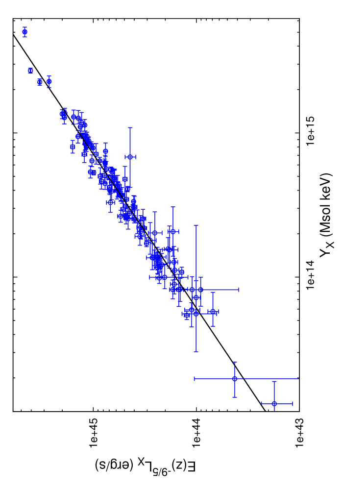
Figure 1.— $\mathrm{L_{X}-Y_{X}}$ relation for bolometric luminosities measured in the $(0.15<r<1)R_{\mathrm{500}}$ aperture. Luminosities are scaled by the predicted self-similar evolution.

Table 1Summary of the best fitting scaling relations between luminosity and $Y_{\mathrm{X}}$, kT, and $M_{\mathrm{500}}$ (the X variables listed in column 1). Luminosities were measured in different apertures, either from spectral fits or from count rates as discussed in the text and listed in columns 2 and 3. The energy bands used for the soft band luminosities are given in the clusters’ rest frames. Relations of the form $L_{\mathrm{X}}=CE(z)^{\alpha}(X/X_{*})^{B}$ were fit to the data with $X_{*}=(6\mbox{$\mathrm{~{}keV}$},4\times 10^{14}\mathrm{M_{\odot}}\mbox{$\mathrm{~{}keV}$},4\times 10^{14}\mathrm{M_{\odot}})$ and $\alpha=(9/5,1,7/3)$ (self-similar evolution) for $Y_{\mathrm{X}}$, kT, and $M_{\mathrm{500}}$ respectively. Column 4 gives the redshift range of the clusters included in the fit. Columns 5 and 6 give the normalisation and slope of the $\mathrm{L_{X}-X}$ relation in question, and columns 7 and 8 give the intrinsic fractional scatter in $L_{\mathrm{X}}$ and X. Masses were estimated from $Y_{\mathrm{X}}$ and the parameters of the best-fitting $\mathrm{L_{X}-M}$ relations include uncertainties and scatter in the $\mathrm{Y_{X}-M_{500}}$ relation.

X	$L_{\mathrm{X}}$ type	$L_{\mathrm{X}}$ aperture	redshift	C	$B$	$\sigma_{L}$	$\sigma_{X}$
				$(10^{44}\mathrm{\mbox{$\mathrm{~{}erg}$}\mathrm{\mbox{$\mathrm{~{}s}$}^{-1}}})$
$Y_{\mathrm{X}}$	spectral, bolometric	$r<R_{\mathrm{500}}$	$0.1<z<1.3$	$10.0\pm 0.4$	$1.10\pm 0.04$	0.36$\pm 0.03$	0.33$\pm 0.03$
$Y_{\mathrm{X}}$	spectral, bolometric	$70\mbox{$\mathrm{~{}kpc}$}<r<R_{\mathrm{500}}$	$0.1<z<1.3$	$8.7\pm 0.2$	$1.06\pm 0.03$	0.21$\pm 0.02$	0.20$\pm 0.01$
$Y_{\mathrm{X}}$	spectral, bolometric	$(0.15<r<1)R_{\mathrm{500}}$	$0.1<z<1.3$	$5.8\pm 0.1$	$0.94\pm 0.03$	0.11$\pm 0.02$	0.12$\pm 0.02$
$Y_{\mathrm{X}}$	spectral, bolometric	$(0.15<r<1)E(z)^{-2/3}\mbox{$\mathrm{~{}Mpc}$}$	$0.1<z<1.3$	$7.0\pm 0.1$	$1.00\pm 0.02$	0.13$\pm 0.02$	0.14$\pm 0.02$
$Y_{\mathrm{X}}$	spectral, $(0.5-2)\mbox{$\mathrm{~{}keV}$}$	$(0.15<r<1)E(z)^{-2/3}\mbox{$\mathrm{~{}Mpc}$}$	$0.1<z<1.3$	$1.85\pm 0.04$	$0.84\pm 0.03$	0.20$\pm 0.01$	0.24$\pm 0.03$
$Y_{\mathrm{X}}$	count rate, $(0.5-2)\mbox{$\mathrm{~{}keV}$}$	$(0.15<r<1)E(z)^{-2/3}\mbox{$\mathrm{~{}Mpc}$}$	$0.1<z<1.3$	$1.91\pm 0.04$	$0.82\pm 0.03$	0.19$\pm 0.01$	0.23$\pm 0.02$
kT	spectral, bolometric	$(0.15<r<1)R_{\mathrm{500}}$	$0.1<z<1.3$	$6.6\pm 0.3$	$2.8\pm 0.2$	0.34$\pm 0.04$	0.12$\pm 0.02$
$M_{\mathrm{500}}$	spectral, bolometric	$r<R_{\mathrm{500}}$	$0.1<z<1.3$	$5.6\pm 0.3$	$1.96\pm 0.10$	0.39$\pm 0.04$	0.21$\pm 0.01$
$M_{\mathrm{500}}$	spectral, bolometric	$(0.15<r<1)R_{\mathrm{500}}$	$0.1<z<1.3$	$3.5\pm 0.1$	$1.63\pm 0.08$	0.17$\pm 0.02$	0.08$\pm 0.02$
$M_{\mathrm{500}}$	count rate, $(0.5-2)\mbox{$\mathrm{~{}keV}$}$	$(0.15<r<1)E(z)^{-2/3}\mbox{$\mathrm{~{}Mpc}$}$	$0.1<z<1.3$	$1.20\pm 0.05$	$1.45\pm 0.07$	0.21$\pm 0.02$	0.16$\pm 0.02$
$M_{\mathrm{500}}$	count rate, $(0.5-2)\mbox{$\mathrm{~{}keV}$}$	$r<1E(z)^{-2/3}\mbox{$\mathrm{~{}Mpc}$}$	$0.1<z<0.5$	$1.7\pm 0.1$	$1.7\pm 0.1$	0.46$\pm 0.05$	0.28$\pm 0.02$
$M_{\mathrm{500}}$	count rate, $(0.5-2)\mbox{$\mathrm{~{}keV}$}$	$r<1E(z)^{-2/3}\mbox{$\mathrm{~{}Mpc}$}$	$0.5<z<1.3$	$1.6\pm 0.1$	$1.5\pm 0.1$	0.19$\pm 0.05$	0.16$\pm 0.04$

3.1. The effect of cooling cores and substructure

In order to test for any residual effects of cooling core emission on the $\mathrm{L_{X}-Y_{X}}$ relation, the sample was split into cool core (CC) and non-cool core (NCC) subsamples. Clusters were classed as CC if the temperature measured within $r<0.15R_{\mathrm{500}}$ was cooler than that measured within $(0.15<r<0.3)R_{\mathrm{500}}$ at a significance of $>2\sigma$. While this method is dependent on the quality of the data used and so is not a robust classification scheme, it allows us to separate out the strongest cool core clusters to look for departures from the population. The relation was fit to the two subsets separately, and the relations are plotted in Fig. 2. There is no evidence for any offset between the CC and NCC populations, though the slope of the CC relation is $\sim 3\sigma$ shallower than the NCC relation. The intrinsic scatter of the 18 CC clusters was $\sigma_{L}=0.04\pm 0.02$, significantly lower than that of the NCC clusters ($\sigma_{L}=0.13\pm 0.02$). This is likely a reflection of the fact that CC clusters are generally more relaxed than the rest of the population. When core emission was not excluded, the CC clusters were significantly offset to higher $L_{\mathrm{X}}$, as expected.

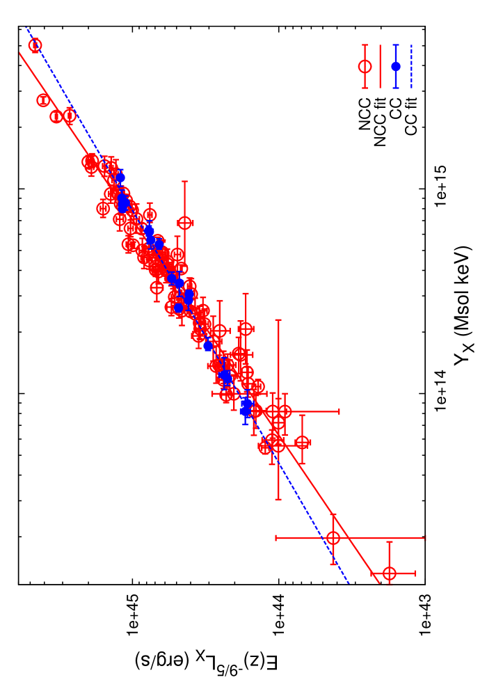
Figure 2.— $\mathrm{L_{X}-Y_{X}}$ relations for cool core (CC) and non-cool core (NCC) clusters. Luminosities are bolometric, measured in the $(0.15<r<1)R_{\mathrm{500}}$ aperture, and scaled by the predicted self-similar evolution.

The sample contains clusters in a wide variety of dynamical states from relaxed, cool core clusters to early and late stage mergers with a range of mass ratios (Maughan et al., 2007). To further investigate the effect of cluster morphology on the $\mathrm{L_{X}-Y_{X}}$ relation, the clusters were split into relaxed and unrelaxed subsamples based on their measured centroid shift ($\langle w\rangle$) parameters (see Maughan et al., 2007, for details). $\langle w\rangle$ was calibrated by visual inspection of cluster images, and the 28 clusters with $\langle w\rangle<0.005R_{\mathrm{500}}$ were classed as relaxed, with the remaining 87 classed as unrelaxed. The $\mathrm{L_{X}-Y_{X}}$ relation was fit to these subsets separately and the data are plotted in Fig. 3. The normalisations were consistent for both subsets, and the slope was slightly shallower ($\sim 1\sigma$) for the relaxed clusters, a similar trend to the CC and NCC clusters. The scatter was slightly, but not significantly, lower for the relaxed clusters. We note that the CC clusters generally have the lowest $\langle w\rangle$, and represent the most relaxed subset of the sample.

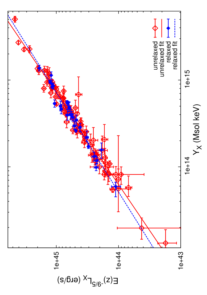
Figure 3.— $\mathrm{L_{X}-Y_{X}}$ relations for relaxed and unrelaxed clusters. Luminosities are bolometric, measured in the $(0.15<r<1)R_{\mathrm{500}}$ aperture, and scaled by the predicted self-similar evolution.

3.2. Evolution

For the previous fits, we assumed that the $\mathrm{L_{X}-Y_{X}}$ relation evolves self-similarly with $a_{LY}=9/5$. We have tested the validity of this assumption by using the data to determine the best-fitting value of $a_{LY}$. For different values of $a_{LY}$, luminosities were divided by $E(z)^{a_{LY}}$, the best fitting relation was found via BCES regression and the $\chi^{2}$ was computed using equation 3 (with $\sigma_{L}=0$). The best-fitting $a_{LY}$ was the value that minimised $\chi^{2}$, and the $1\sigma$ confidence intervals were given by the values that gave $\Delta\chi^{2}=1$ from the minimum.

The best-fitting evolution was $a_{LY}=2.2\pm 0.1$, significantly ($4\sigma$) higher than the self-similar value. To illustrate the evolution, a local $\mathrm{L_{X}-Y_{X}}$ relation was defined by fitting the 20 clusters at $0.1<z<0.2$. Self-similar evolution was assumed for measuring this local relation, though the effect at these low redshifts is small. The ratio of a cluster’s measured luminosity to that predicted by this local relation for the cluster’s $Y_{X}$ is then equal to $E(z)^{a_{LY}}$. Fig. 4 shows the value of this ratio for each cluster along with the loci of the self-similar and best-fitting evolution.

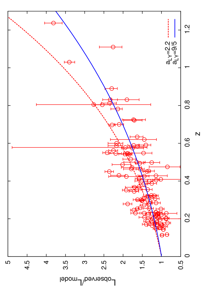
Figure 4.— Ratio of the observed $L_{X}$ to that predicted by the local $\mathrm{L_{X}-Y_{X}}$ relation is plotted against redshift. The curves show the predicted self-similar (solid) and best-fitting (dashed) evolution.

While the data prefer a stronger evolution than the self-similar prediction, both evolution models give an unacceptable fit ($\chi^{2}/\nu\approx 4$). This is a result of the significant intrinsic scatter in the data; both evolution models require $\sigma_{L}=0.11$ to give a reduced $\chi^{2}$ of unity. Without a priori knowledge of the details of this scatter that would allow us to distinguish between evolution models, we find no compelling reason to abandon the theoretically motivated self-similar evolution, and continue to adopt it throughout this work.

3.3. Survey-quality data

The tight correlation between $L_{\mathrm{X}}$ and $Y_{\mathrm{X}}$ and that between $Y_{\mathrm{X}}$ and mass (KVN06) suggests that $L_{\mathrm{X}}$ can provide an effective mass proxy. However, data that are of sufficient quality ($\sim 1000$ net counts) to allow a spectrum to be fit and a luminosity measured in that way, will generally allow $Y_{\mathrm{X}}$ to be measured directly (as is the case for our sample). The prospect of estimating masses reliably from luminosities has much greater potential for clusters detected in serendipitous cluster surveys, where only count rates are available. We now investigate how well the $\mathrm{L_{X}-Y_{X}}$ relation holds up for such relatively low-quality data.

Up to this point, $Y_{\mathrm{X}}$ has weakly influenced our $L_{\mathrm{X}}$ measurements, as $R_{\mathrm{500}}$ (and hence the luminosity aperture) was estimated from $Y_{\mathrm{X}}$. This dependence was removed by switching to an aperture of $(0.15<r<1)E(z)^{-2/3}\mbox{$\mathrm{~{}Mpc}$}$, chosen to approximate $(0.15<r<1)R_{\mathrm{500}}$. Encouragingly, the scatter in the $\mathrm{L_{X}-Y_{X}}$ relation was insensitive to this change, with $\sigma_{L}=0.13\pm 0.02$. Next, the energy band of the luminosities measured from the spectral fits was changed from the bolometric band to the $(0.5-2)\mbox{$\mathrm{~{}keV}$}$ band in each cluster’s rest frame. This change was motivated by the fact that the soft band $L_{\mathrm{X}}$ is less sensitive to the cluster temperature than the bolometric band, so can be more reliably estimated from a soft band count rate (typical of survey data) without a measured temperature. The soft band $\mathrm{L_{X}-Y_{X}}$ relation showed slightly increased scatter ($\sigma_{L}=0.21\pm 0.02$) likely due to the fact that the increased temperature dependence of the bolometric $L_{\mathrm{X}}$ suppresses the scatter somewhat, since $Y_{\mathrm{X}}$ is proportional to temperature.

Finally, for each cluster we measured the net count rate in the observed frame $(0.5-2)\mbox{$\mathrm{~{}keV}$}$ band, and converted it to a rest frame $(0.5-2)\mbox{$\mathrm{~{}keV}$}$ luminosity. For the conversion we assumed an absorbed APEC spectral model with the absorption fixed at the galactic value for each cluster, the redshift fixed at that of the cluster, and metal abundance fixed at $0.3\mathrm{Z_{\odot}}$. The temperature of the spectral model was set at an initial guess and $L_{\mathrm{X}}$ was calculated. A luminosity-temperature relation was then used to estimate $kT$ from $L_{\mathrm{X}}$ and the process was iterated until $L_{\mathrm{X}}$ stabilised. The Markevitch (1998) $\mathrm{L_{X}-kT}$ relation was used, with self-similar evolution, but the conversion is insensitive to the choice of $\mathrm{L_{X}-kT}$ relation. The reliability of this conversion was verified by comparing our estimated luminosities with those measured from the spectral fits, and an excellent agreement was found (illustrated in Fig. 5). The $\mathrm{L_{X}-Y_{X}}$ relation was then measured using these estimated soft band luminosities, and the scatter did not change significantly $\sigma_{L}=0.19\pm 0.01$.

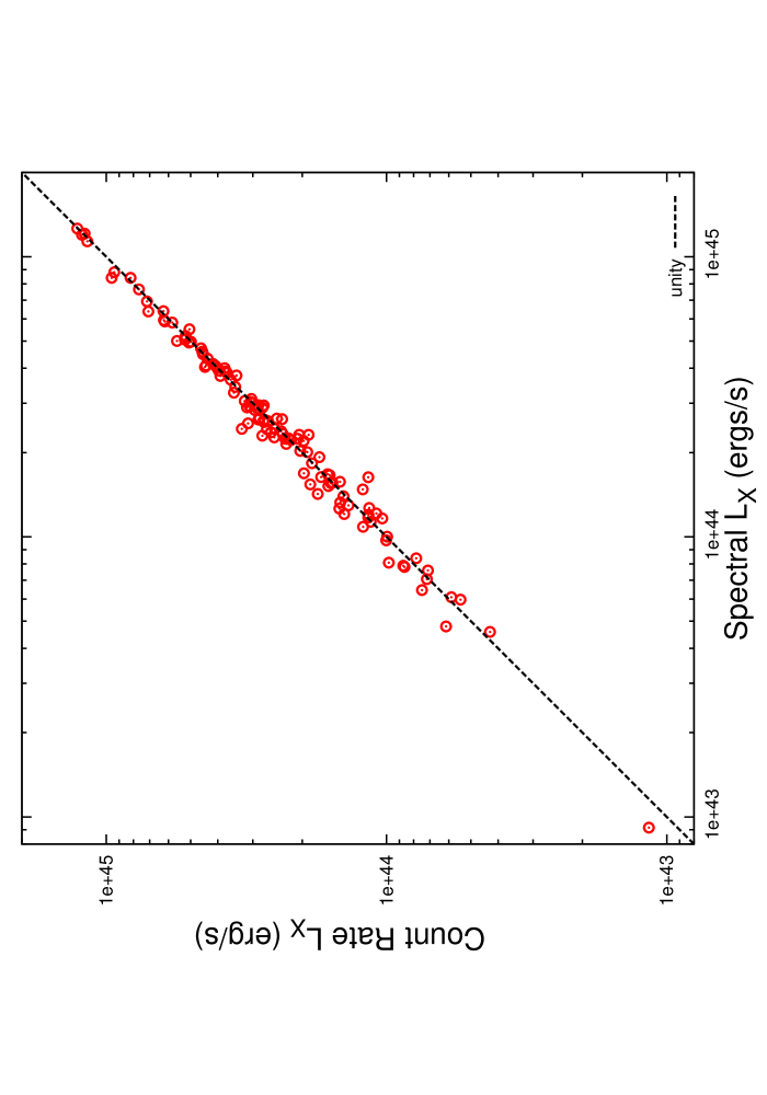
Figure 5.— The rest-frame $(0.5-2.0)\mbox{$\mathrm{~{}keV}$}$ luminosity measured from a full spectral fit is plotted against the luminosity estimated from the count rate in the same energy band. The $(0.15<r<1)E(z)^{-2/3}\mbox{$\mathrm{~{}Mpc}$}$ aperture was used for both measurements and the dashed line indicates a one-to-one correspondence.

4. The $\mathrm{Y_{X}-M_{500}}$ relation

The ultimate goal of this study is to investigate the $\mathrm{L_{X}-M_{500}}$ relation using $Y_{\mathrm{X}}$ as a mass proxy. The use of $Y_{\mathrm{X}}$ as a low-scatter mass proxy has strong support from simulations (KVN06 Poole et al., 2007), but there have not yet been many observational studies of this parameter. The $\mathrm{Y_{X}-M_{500}}$ relation measured for the V06 clusters exhibits the same low scatter found in the simulated relation (KVN06), but the predicted self-similar evolution of the relation has not yet been tested observationally. It is therefore desirable to investigate the scatter and evolution of the $\mathrm{Y_{X}-M_{500}}$ relation using clusters from our sample. This requires independent mass estimates for for the clusters. These can be estimated from temperature and gas density profiles measured from X-ray observations, assuming hydrostatic equilibrium. However, data of sufficient quality are unavailable for the majority of our sample, and a full mass analysis of the remainder is beyond the scope of the current work. Instead, we searched the literature for mass estimates for clusters in our sample. We found 12 clusters in our sample with values of $M_{\mathrm{500}}$ estimated from full X-ray hydrostatic mass analyses (i.e. using temperature and density profiles rather than an isothermal approximation). Masses for 3 clusters were taken from the overlap between our sample and the V06 sample, one was obtained from the XMM-Newton sample of Arnaud et al. (2005), and the remainder came from the XMM-Newton and Chandra samples presented by Kotov & Vikhlinin (2005) and Kotov & Vikhlinin (2006) respectively. The properties of the clusters are summarised in Table 2.

Table 2Properties of the subset of clusters with masses based on high quality data available in the literature. Masses were estimated using X-ray hydrostatic mass analyses within $R_{\mathrm{500}}$. The luminosities and $Y_{\mathrm{X}}$ values presented were measured from our analyses, with $L_{\mathrm{X}}$ measured in the $(0.15<r<1)R_{\mathrm{500}}$ aperture. The references for the mass estimates listed in column 6 correspond to: 1 - Vikhlinin et al. (2006), 2 - Arnaud et al. (2005), 3 - Kotov & Vikhlinin (2005), 4 - Kotov & Vikhlinin (2006).

Cluster	z	$L_{\mathrm{X}}$	$Y_{\mathrm{X}}$	$M_{\mathrm{500}}$	Reference
		$(10^{44}\mathrm{\mbox{$\mathrm{~{}erg}$}\mathrm{\mbox{$\mathrm{~{}s}$}^{-1}}})$	$(10^{14}\mathrm{M_{\odot}}\mbox{$\mathrm{~{}keV}$})$	$(10^{14}\mathrm{M_{\odot}})$
A1413	0.143	$7.6\pm 0.1$	$5.6\pm 0.2$	$7.8\pm 0.8$	1
A907	0.153	$4.7\pm 0.1$	$3.0\pm 0.1$	$4.7\pm 0.4$	1
A383	0.187	$3.6\pm 0.1$	$1.7\pm 0.1$	$3.1\pm 0.3$	1
A2204	0.152	$12.7\pm 0.3$	$8.9\pm 0.7$	$8.4\pm 0.8$	2
MS0302.7+1658	0.424	$3.0\pm 1.2$	$9.2\pm 1.5$	$2.2\pm 0.6$	3
MS0015.9+1609	0.541	$33.9\pm 0.6$	$13.4\pm 1.0$	$8.8\pm 1.1$	3
CLJ1120+4318	0.600	$8.3\pm 0.7$	$2.5\pm 0.6$	$4.6\pm 1.1$	3
MACSJ0159.8-0849	0.405	$17.7\pm 0.3$	$11.2\pm 1.1$	$9.9\pm 3.1$	4
MACSJ0329.6-0211	0.450	$11.3\pm 0.6$	$3.3\pm 0.4$	$3.6\pm 1.0$	4
RXJ1347.5-1145	0.451	$41.4\pm 0.8$	$2.4\pm 0.2$	$13.8\pm 2.8$	4
MACSJ1621.3+3810	0.463	$8.5\pm 0.5$	$3.8\pm 0.4$	$4.4\pm 1.0$	4
MACSJ1423.8+2404	0.543	$11.3\pm 0.7$3	$4.1\pm 0.7$	$4.6\pm 1.0$	4

The $\mathrm{Y_{X}-M_{500}}$ relation for these 12 clusters is shown in Fig. 6. It was constructed using our measured $Y_{\mathrm{X}}$ values, with the masses taken from the literature and scaled by the predicted self-similar evolution ($E(z)^{2/5}$). These data were compared with the best fit relation to the V06 clusters (equation 1), with which three clusters are in common. The V06 relation is a good description of the data; the reduced $\chi^{2}$ is $<1$ so there is no measurable intrinsic scatter. While the intrinsic scatter cannot be well constrained with this small sample, the tight correlation in Fig. 6 adds further support to the use of $Y_{\mathrm{X}}$ as a low-scatter mass proxy, and provides the first observational support for the self-similar evolution of the $\mathrm{Y_{X}-M_{500}}$ relation to $z=0.6$.

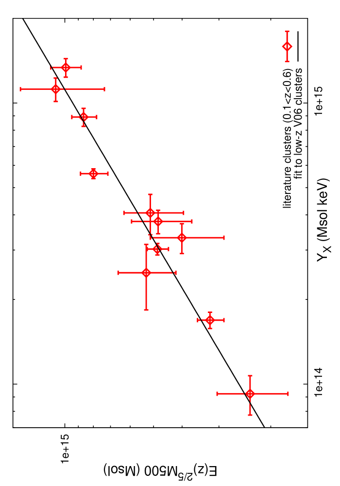
Figure 6.— $\mathrm{Y_{X}-M_{500}}$ relation using our measured $Y_{\mathrm{X}}$ values with masses taken from the literature. The masses are scaled by the expected self-similar evolution. The line shows the best fit to the V06 data; this line is not fit to the data plotted here, but 3 of the datapoints are in common with the V06 sample.

5. Estimating masses from luminosities

As a final exercise, we use the $\mathrm{Y_{X}-M_{500}}$ relation to estimate masses for the clusters in the sample, and then investigate the $\mathrm{L_{X}-M_{500}}$ relation using luminosities measured in different ways. In order to include the effects of both the intrinsic scatter and the uncertainties on the $\mathrm{Y_{X}-M_{500}}$ relation on our derived $\mathrm{L_{X}-M_{500}}$ relation, we used a Monte-Carlo approach as follows. A random realisation of the $\mathrm{Y_{X}-M_{500}}$ relation (equation 1) was created by drawing values of the slope and normalisation from the Gaussian distributions defined by $B_{YM}=0.564\pm 0.009$ and $C_{YM}=(7.047\pm 0.097)\times 10^{14}\mathrm{M_{\odot}}$. These are the best-fitting values from the V06 data, but with the errors taken from the fractional errors on the KVN06 simulated relation. For each cluster, a mass was computed using this relation (assuming self-similar evolution) and that mass was then randomised under a Gaussian in natural log space centred at the true value with $\sigma=0.071$. This corresponds to the $7.1\%$ intrinsic scatter in mass in the $\mathrm{Y_{X}-M_{500}}$ relation found by KVN06.

The $\mathrm{L_{X}-M_{500}}$ relation was then fit using these randomised masses and our measured luminosities. The process was repeated 1000 times and the distributions of measured slope ($B_{LM}$), normalisation ($C_{LM}$) and scatter in $\mathrm{L_{X}-M_{500}}$ were then used to determine the values and uncertainties of those parameters. The uncertainties and scatter in the $\mathrm{Y_{X}-M_{500}}$ relation did not contribute strongly to those on the derived $\mathrm{L_{X}-M_{500}}$ relations. In all cases, the $\pm 34$ percentiles about the mean of the $B_{LM}$ and $C_{LM}$ distributions derived from the Monte-Carlo randomisations enclosed a smaller range than the statistical uncertainties from the regression fit to the unperturbed $\mathrm{L_{X}-M_{500}}$ relation. The Monte-Carlo uncertainties were added in quadrature to the regression uncertainties to give the final uncertainties for these parameters. We used the median and $\pm 34$ percentiles of the distribution of $\sigma_{L}$ from the Monte-Carlo runs as our estimate of the scatter in the $\mathrm{L_{X}-M_{500}}$ relation. This too was not strongly affected by the scatter in $\mathrm{Y_{X}-M_{500}}$; the median $\sigma_{L}$ was $\,\hbox to0.0pt{\raise 1.72218pt\hbox{$<$}\hss}{\lower 2.58334pt\hbox{$\sim$}}\,0.03$ higher than that measured for the unperturbed $\mathrm{L_{X}-M_{500}}$ data in all cases. The measured $\mathrm{L_{X}-M_{500}}$ relations are summarised in Table 1 and the relation obtained for bolometric $L_{\mathrm{X}}$ measured from spectral fits in the $(0.15<r<1)R_{\mathrm{500}}$ aperture is plotted in Fig. 7. As expected, the scatter follows the same trend as in the $\mathrm{L_{X}-Y_{X}}$ relation, reducing from $0.39\pm 0.04$ to $0.17\pm 0.02$ when the core regions were fully excluded, with a slightly larger scatter of $\sigma_{L}=0.21\pm 0.02$ for survey-quality data.

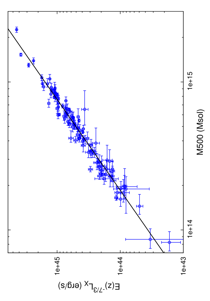
Figure 7.— $\mathrm{L_{X}-M_{500}}$ relation for the clusters with masses estimated from the $\mathrm{Y_{X}-M_{500}}$ relation and bolometric luminosities measured from spectral fits in the $(0.15<r<1)R_{\mathrm{500}}$ aperture, and scaled by the predicted self-similar evolution.

5.1. Correlation of scatter in the $\mathrm{L_{X}-Y_{X}}$ and $\mathrm{Y_{X}-M_{500}}$ relations.

Our Monte-Carlo method assumes that the scatter in the $\mathrm{L_{X}-Y_{X}}$ and $\mathrm{Y_{X}-M_{500}}$ relations is uncorrelated. If they were positively or negatively correlated, then the derived scatter on the $\mathrm{L_{X}-M_{500}}$ relation would be under- or overestimated respectively. Ideally, one would measure the offset of clusters in $L_{\mathrm{X}}$ from the $\mathrm{L_{X}-Y_{X}}$ relation ($\delta_{LY}$) and in $Y_{\mathrm{X}}$ from the $\mathrm{Y_{X}-M_{500}}$ relation ($\delta_{YM}$) and test for correlations between those offsets. This is not possible for the full sample, as independent mass estimates are not available, but this can be investigated for the subset of clusters with masses taken from the literature. The offsets for these clusters are plotted in Fig. 8. The data hint at a positive correlation, but the correlation is not significant if the uncertainties on the data points are included.

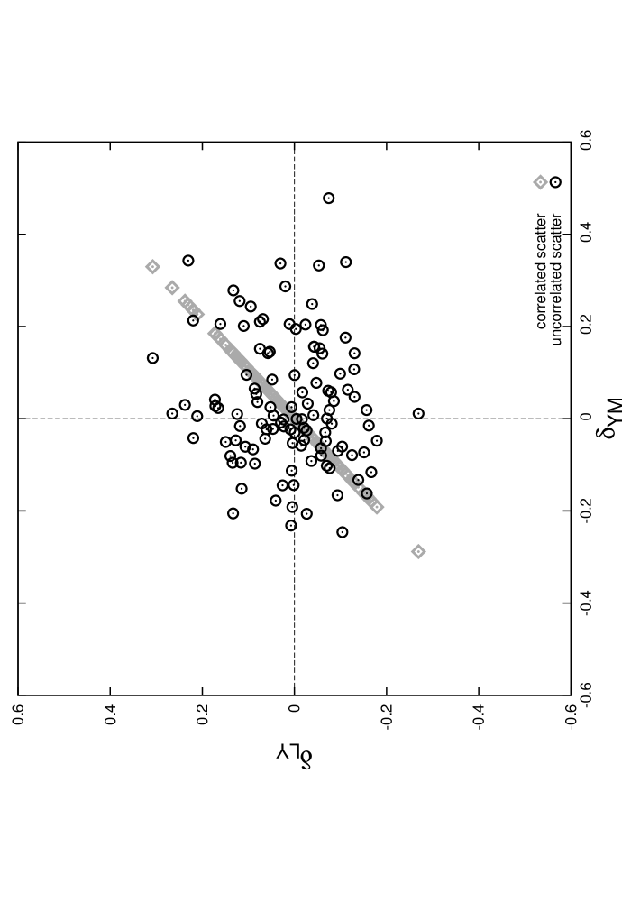
Figure 8.— Left: Fractional residuals in $L_{\mathrm{X}}$ from the $\mathrm{L_{X}-Y_{X}}$ relation ($\delta_{LY}$) and in $Y_{\mathrm{X}}$ from the $\mathrm{Y_{X}-M_{500}}$ relation ($\delta_{YM}$) for the subset of clusters with mass estimates taken from the literature. Right: The same residuals for the full sample from one of the Monte-Carlo runs for the assumptions of correlated and uncorrelated scatter in the $\mathrm{L_{X}-Y_{X}}$ and $\mathrm{Y_{X}-M_{500}}$ relations.

In order to investigate the case of positive correlation between the scatter in the $\mathrm{L_{X}-Y_{X}}$ and $\mathrm{Y_{X}-M_{500}}$ relations and thus place a conservative upper limit on the $\mathrm{L_{X}-M_{500}}$ scatter, we rederived the $\mathrm{L_{X}-M_{500}}$ relation assuming that $\delta_{LY}$ and $\delta_{YM}$ are perfectly correlated. In this process, cluster masses were estimated using the $\mathrm{Y_{X}-M_{500}}$ relation as before, but were then scattered to give a $\delta_{YM}$ that was proportional to the cluster’s known $\delta_{LY}$. The constant of proportionality used was the ratio of the scatter in the $\mathrm{L_{X}-Y_{X}}$ and $\mathrm{Y_{X}-M_{500}}$ relations. This is illustrated in Fig. 8 along with an example of uncorrelated scatter as assumed previously. With this assumption of correlated scatter, the resulting scatter in the $\mathrm{L_{X}-M_{500}}$ relation for $L_{\mathrm{X}}$ measured from spectral fits in the $(0.15<r<1)R_{\mathrm{500}}$ aperture increased from $\sigma_{L}=0.17\pm 0.02$ to $\sigma_{L}=0.23\pm 0.02$. For comparison, the $\mathrm{L_{X}-M_{500}}$ relation was also constructed for the subset of 12 clusters with independent mass estimates from the literature, using our measured luminosities in the $(0.15<r<1)R_{\mathrm{500}}$ aperture. The scatter of these data about the $\mathrm{L_{X}-M_{500}}$ relation derived for the full sample was found to be $\sigma_{L}=0.19\pm 0.11$. The large uncertainties on the scatter due to the small number of clusters with independent mass measurements limit our ability to pin down the extent of the correlation between $\delta_{LY}$ and $\delta_{YM}$, and the precise value of the scatter in the $\mathrm{L_{X}-M_{500}}$ relation. This will be addressed in future work by deriving masses for a larger subset of our sample. In the mean time, we continue with the assumption of uncorrelated scatter, but the increase in $\sigma_{L}$ for correlated scatter indicates the size of any sytematic effect due to this assumption.

5.2. The effect of including core emission for high-z clusters

A source of concern for the application of this method is that a substantial fraction of the cluster emission is excluded by excluding the cluster core out to $0.15R_{\mathrm{500}}$ (or $0.15E(z)^{-2/3}\mbox{$\mathrm{~{}Mpc}$}$). To quantify this, we compared the flux measured from spectral fits in the $(0.15<r<1)R_{\mathrm{500}}$ aperture and the total flux within $R_{\mathrm{500}}$ after correction for cool cores. The standard cool-core correction of multiplying the flux measured in the $70\mbox{$\mathrm{~{}kpc}$}<r<R_{\mathrm{500}}$ aperture by $1.06$ was used (Markevitch, 1998). The mean ratio of the $(0.15<r<1)R_{\mathrm{500}}$ to total flux was $0.70$, so typically $30\%$ of the flux is excluded. A second issue is that for telescopes with a significant point spread function (PSF) such as ROSAT and XMM-Newton, the central exclusion region becomes smaller than the PSF for distant clusters, making core exclusion difficult.

Recently (Vikhlinin et al., 2006) used measurements of the gas density profile slopes in the cores of galaxy clusters to show that the fraction of clusters with cool cores is low at $z\gtrsim 0.5$. As cool cores are the dominant source of scatter in these scaling relations, it is therefore interesting to measure the scatter without core exclusion for distant clusters to determine if it can be neglected for high-z clusters. Luminosities were estimated from count rates in the $r<1E(z)^{-2/3}\mbox{$\mathrm{~{}Mpc}$}$ aperture (i.e. including core emission) and the sample was split at $z=0.5$ into low- and high-redshift subsets. The $\mathrm{L_{X}-M_{500}}$ relation was calculated for each subset as described above, and the parameters are given in Table 1. The best-fitting relations are consistent for the two subsets, but the scatter for the low redshift subset ($\sigma_{L}=0.46\pm 0.05$) is significantly larger than that for the high-z clusters ($\sigma_{L}=0.19\pm 0.05$). In fact, the scatter for the distant clusters with the cores included is the same as that for the full sample with cores excluded. This suggests that the core exclusion is generally not required for clusters at $z>0.5$. Note that while the measurement errors are generally larger for the more distant clusters, these values for the intrinsic scatter take those into account.

6. Discussion

Table 1 shows that the scatter in the scaling relations is dominated by the cluster core regions. The obvious candidate is the enhanced $L_{\mathrm{X}}$ due to cool cores. However, it should be noted that the strongest effects of mergers on $L_{\mathrm{X}}$ occur around core passage of the merging bodies (e.g. Randall et al., 2002). By excluding a large core region, we also effectively remove the strongest part of the scatter due to mergers. The scatter from the core regions is thus due to a combination of mergers and cooling. Once the core regions are excised, the morphological status of the clusters has little effect on the scatter unless only the most relaxed systems (the CC clusters) are considered (§3.1). The total intrinsic scatter of $\sigma_{L}=0.36$ in the $\mathrm{L_{X}-Y_{X}}$ relation can thus be resolved into different components. The total scatter reduces by $\approx 70\%$ when the central $0.15R_{\mathrm{500}}$ is excluded. A further $\approx 20\%$ of the scatter is removed when only the most relaxed CC systems are considered; this portion of the scatter is likely due to merger effects outside the cores. The remaining $\approx 10\%$ of the scatter is likely due to residual substructure even in the most relaxed systems, to the scatter in the $\mathrm{Y_{X}-M_{500}}$ relation, which has a weak effect on our measured luminosities through $R_{\mathrm{500}}$, and to contributions from unresolved point sources.

For comparison with the $\mathrm{L_{X}-Y_{X}}$ relation, we also measured the $\mathrm{L_{X}-kT}$ relation for the sample, using luminosities and temperatures measured in the $(0.15<r<1)R_{\mathrm{500}}$ aperture. The best fit parameters are given in Table 1, but the main point to note is that even with our most conservative core exclusion, $\sigma_{L}$ in the $\mathrm{L_{X}-kT}$ relation is three times that in the corresponding $\mathrm{L_{X}-Y_{X}}$ relation. The fact that $Y_{\mathrm{X}}$ has been shown to be a low-scatter mass proxy implies that the larger scatter in the $\mathrm{L_{X}-kT}$ relation is due to scatter in the $\mathrm{M-kT}$ relation. As our mass estimates are based on kT (via $Y_{\mathrm{X}}$), we cannot investigate the scatter in the $\mathrm{M-kT}$ relation for our sample. However, our results suggest that for samples such as ours, which include relaxed and disturbed clusters, luminosity (with a large core region excluded) has a tighter relation with mass than temperature does. Although, recall that $Y_{\mathrm{X}}$ has a tighter relation with mass than do either $L_{\mathrm{X}}$ or kT. Clusters with strong deviations from the $\mathrm{L_{X}-kT}$ relation will be studied in detail in a future paper.

6.1. The shape of the scatter in the $\mathrm{L_{X}-Y_{X}}$ relation

It is desirable to adopt a functional form for the intrinsic scatter in the scaling relations in order to include its effects on e.g. sample completeness and derived mass functions. With 115 clusters it is possible to investigate the form of the scatter in the $\mathrm{L_{X}-Y_{X}}$ relation. Fig. 9 shows a histogram of the $\log_{e}$ space residuals from the $\mathrm{L_{X}-Y_{X}}$ relation fit to all clusters, using spectral $L_{\mathrm{X}}$ measured in the $(0.15<r<1)R_{\mathrm{500}}$ aperture. This raw scatter is well described by a Gaussian in log space with $\sigma_{L}=0.19$; a Kolmogorov-Smirnov test gives a null hypothesis probability of $0.99$ that the data are consistent with that Gaussian. Here we have implicitly assumed that the scatter does not vary with redshift.

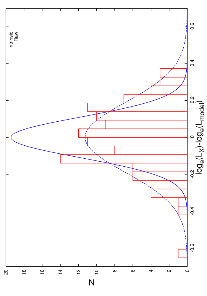
Figure 9.— Histogram of the residuals from the $\mathrm{L_{X}-Y_{X}}$ relation in $\log_{e}$ space. This raw scatter is well described by a Gaussian of $\sigma_{L}=0.19$ (dashed line). The solid line is a Gaussian with $\sigma_{L}=0.11$ corresponding to the measured intrinsic scatter.

The form of the intrinsic scatter is harder to recover. For each cluster we have an observed luminosity ($L_{\mathrm{X}}$) and a luminosity predicted by the $\mathrm{L_{X}-Y_{X}}$ relation for that clusters measured $Y_{\mathrm{X}}$ ($L_{model}$). Each log space residual ($\log_{e}(L_{\mathrm{X}}/L_{model})$) is associated with a measurement error on ($L_{\mathrm{X}}/L_{model}$), which we assume is described by a Gaussian distribution in linear space. The raw scatter can then be approximated as a convolution of the intrinsic scatter distribution with a linear Gaussian representing the mean measurement error on the residuals. This approximation was used to test if the intrinsic scatter could be described by a lognormal distribution. A simulated residual point was drawn from under a Gaussian with $\sigma=0.11$ in log space (our intrinsic scatter model). This value of $\log_{e}(L_{\mathrm{X}}/L_{model})$ was transformed into linear space ($L_{\mathrm{X}}/L_{model}$) and then randomised under a Gaussian of $\sigma=0.17$ (the mean measurement error on $L_{\mathrm{X}}/L_{model}$). Note that we verified that the measurement errors on $L_{\mathrm{X}}/L_{model}$ were not significantly correlated with $L_{\mathrm{X}}/L_{model}$. This was repeated for $10,000$ simulated residuals to give a simulated raw scatter distribution. The resulting distribution was compared to the observed raw scatter distribution using the Kolmogorov-Smirnov test, and the cumulative probability distributions are plotted in Fig. 10. The distributions agree very well, with a null hypothesis probability of $0.91$, indicating that the intrinsic scatter is well described by a lognormal distribution.

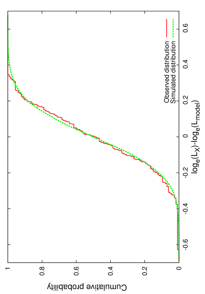
Figure 10.— Cumulative probability distributions for the observed (solid line) and simulated (dashed line) raw scatter.

6.2. The effect of Eddington bias

An important factor that we have not yet addressed is the issue of Eddington bias. In a flux-limited sample, clusters of a range of masses that have fluxes near the detection limit are scattered into and out of the sample, due to the intrinsic scatter in cluster luminosities for a given mass. Because the mass function is a decreasing function of mass, more clusters will scatter into than out of the sample. This results in a bias in both the number of clusters and their mean luminosities (as clusters with above average luminosities will be over-represented). The magnitude of the bias depends on the amount of scatter in the $\mathrm{L_{X}-M}$ relation and on the slope of the mass function around the flux limit (that is, the mass limit corresponding to the flux limit when converted to a luminosity at the redshift of interest) of the sample. As the mass function steepens at higher masses, surveys with higher mass limits will suffer a larger bias. The bias can affect the slope, normalisation, evolution and scatter of the scaling relations measured with the sample.

The heterogeneous nature of our sample, with clusters drawn from a variety of different samples, makes it difficult to quantify the effects of the Eddington bias on the scaling relations. To illustrate this, consider three surveys (all based on ROSAT data) that are represented (incompletely) in our sample are the Brightest Cluster Survey (BCS; Ebeling et al., 1998) covering $z\lesssim 0.3$, the Massive Cluster Survey (MACS; Ebeling et al., 2001) at $0.3\lesssim z\lesssim 0.6$, and the 400 Square Degree survey (400SD; Burenin et al., 2006) at $0.3\lesssim z\lesssim 1$. The flux limits of these surveys correspond to masses (within $R_{\mathrm{500}}$) of approximately $5\times 10^{14}\mathrm{M_{\odot}}$ (BCS at $z=0.2$), $7\times 10^{14}\mathrm{M_{\odot}}$ (MACS at $z=0.45$), $3\times 10^{14}\mathrm{M_{\odot}}$ (400SD at $z=0.7$). The bias thus varies across our sample, and is lowest for the deeper surveys. As a simple test of the effect of the bias on the measured evolution, the evolution was fit to the $z>0.6$ clusters alone. These clusters are generally drawn from deep surveys for which the bias is lower. The best fitting evolution was $a_{LY}=2.0\pm 0.1$, lower than the value measured using the whole sample ($a_{LY}=2.2\pm 0.1$), and approaching the self-similar value of $1.8$. This indicates that stronger than self-similar evolution measured for the whole sample (§3.2) is due in part to the effects of bias. However, it should be noted that the evolution is measured with respect to a local relation, which is itself affected by Eddington bias at some level. The low scatter in the $\mathrm{L_{X}-Y_{X}}$ relation means that the effects of bias should be fairly small, but these will be quantified using statistically complete samples at high and low redshifts in a future study.

6.3. Comparison with other measurements of scatter in the $\mathrm{L_{X}-M}$ relation.

The scatter we find in the $\mathrm{L_{X}-M_{500}}$ relation ($\sigma_{L}=0.17-0.39$) is significantly lower than that measured by RB02 who found a total (statistical and intrinsic) scatter of $0.74$ in a sample of $106$ nearby clusters (we refit their data to measure the intrinsic scatter alone, and found $\sigma_{L}=0.63$). Several important differences exist between that work and our study. RB02 used luminosities including the entire core region, derived masses from cluster temperatures assuming isothermality, and finally, derived the masses used for the scatter measurement within $R_{\mathrm{200}}$, rather than our $R_{\mathrm{500}}$. Indeed, for our sample, we find $\sigma_{L}=0.39$ when all of the core emission is included in our $L_{\mathrm{X}}$ measurements (see Table 1), suggesting that the remaining difference from the RB02 is due to the scatter in the $\mathrm{M-kT}$ relation used to derive their masses.

Other recent work has also shown that the scatter in the $\mathrm{L_{X}-M}$ relation is lower than previously thought. Reiprich (2006) and Stanek et al. (2006) compared theoretical mass functions with the X-ray luminosity function measured from the RB02 data to determine the scatter in the $\mathrm{L_{X}-M}$ relation. The measured scatter depends strongly on the assumed cosmology, through the dependence of the mass function on $\sigma_{8}$ and $\Omega_{m}$. Using the best-fitting cosmological values from the WMAP year 3 results ($\sigma_{8}=0.74$, $\Omega_{m}=0.238$; Spergel et al., 2006), Reiprich (2006) concluded that the scatter is small (but non-zero). Stanek et al. (2006) showed that assuming the WMAP year 1 cosmology ($\sigma_{8}=0.9$, $\Omega_{m}=0.29$; Spergel et al., 2003) results in a large scatter in the $\mathrm{L_{X}-M}$ relation and suggested a compromise model with $\sigma_{8}=0.85$ and $\Omega_{m}=0.24$ that gives a scatter of $0.21$ in $M_{\mathrm{200}}$ for a given $L_{\mathrm{X}}$. The measurement from our sample that is most directly comparable to this value is the scatter in $M_{\mathrm{500}}$ for $L_{\mathrm{X}}$ measured with the cluster cores included, $\sigma_{M}=0.21$. This is in agreement with the Stanek et al. (2006) “compromise cosmology” value and is within the $90\%$ upper limit on the scatter set by Reiprich (2006) using the WMAP year 3 cosmology (estimated by converting their upper limit on the bias factor to a scatter). Note that we do not suggest that the scatter measured with our data can be used to distinguish between different cosmological models.

7. Conclusions

We have used a sample of $115$ clusters of $M_{\mathrm{500}}\gtrsim 10^{14}\mathrm{M_{\odot}}$ spanning the redshift range $0.1<z<1.3$ to study the $\mathrm{L_{X}-Y_{X}}$ relation, and by proxy, the $\mathrm{L_{X}-M_{500}}$ relation. We verified the low scatter in the $\mathrm{Y_{X}-M_{500}}$ relation and its self-similar evolution to $z=0.6$ for clusters in our sample using mass estimates from the literature. Our main conclusions are as follows.

• A strong correlation exists between $L_{\mathrm{X}}$ and $Y_{\mathrm{X}}$.

• The scatter in the $\mathrm{L_{X}-Y_{X}}$ (and hence $\mathrm{L_{X}-M_{500}}$) relations is dominated by cluster cores, with a secondary contribution from the less relaxed systems at larger radii.

• Once a sufficiently large core region is excluded ($0.15R_{\mathrm{500}}$ or $0.15E(z)^{-2/3}\mbox{$\mathrm{~{}Mpc}$}$) the scatter in the $\mathrm{L_{X}-Y_{X}}$ relation, and by proxy $\mathrm{L_{X}-M_{500}}$ relation are low ($11\%$ and $17\%$ respectively).

• The scatter remains reasonably small for survey-quality data, where $L_{\mathrm{X}}$ is estimated from soft band count rates, increasing to $19\%$ ($\mathrm{L_{X}-Y_{X}}$) and $21\%$ ($\mathrm{L_{X}-M_{500}}$).

• The slope and normalisation of the $\mathrm{L_{X}-Y_{X}}$ (and by proxy $\mathrm{L_{X}-M_{500}}$) relation are insensitive to the merger status of the clusters, although the scatter can be further reduced by considering only the most relaxed clusters.

• The shape of the intrinsic scatter distribution about the $\mathrm{L_{X}-Y_{X}}$ relation is well described by a lognormal function.

• The evolution of the $\mathrm{L_{X}-Y_{X}}$ relation appears consistent with the self-similar prediction, though our lack of knowledge of the details of the scatter and Eddington bias limit the strength of this conclusion.

• The inferred scatter in $\mathrm{L_{X}-M_{500}}$ is much smaller than that found by previous studies because of i) our improved mass estimates using $Y_{\mathrm{X}}$, and ii) our conservative exclusion of core emission. This is consistent with recent results by Reiprich (2006) and Stanek et al. (2006).

• For high-redshift ($z>0.5$) clusters, there is no need to exclude the core emission. The scatter for high-z clusters with cores included is the same as that measured for the entire sample with cores excluded. This is likely due to the absence of cool core clusters at high redshifts (Vikhlinin et al., 2006).

These results suggest that a simple luminosity measurement can provide an effective mass proxy for clusters with low-quality data (i.e.  insufficient to measure $Y_{\mathrm{X}}$ directly) out to high redshifts. This has important applications for testing cosmological models with current and future X-ray cluster surveys.

References

- Akritas & Bershady (1996) Akritas M. G., Bershady M. A., 1996, ApJ, 470, 706
- Allen et al. (2004) Allen S. W., Schmidt R. W., Ebeling H., Fabian A. C., van Speybroeck L., 2004, MNRAS, 353, 457
- Arnaud & Evrard (1999) Arnaud M., Evrard A. E., 1999, MNRAS, 305, 631
- Arnaud et al. (2005) Arnaud M., Pointecouteau E., Pratt G. W., 2005, A&A, 441, 893
- Böhringer et al. (2001) Böhringer H., Schuecker P., Guzzo L., Collins C. A., Voges W., Schindler S., Neumann D. M., Cruddace R. G., De Grandi S., Chincarini G., Edge A. C., MacGillivray H. T., Shaver P., 2001, A&A, 369, 826
- Burenin et al. (2006) Burenin R. A., Vikhlinin A., Hornstrup A., Ebeling H., Quintana H., Mescheryakov A., 2006, ArXiv Astrophysics e-prints
- Chen et al. (2007) Chen Y., Reiprich T. H., Böhringer H., Ikebe Y., Zhang Y. ., 2007, ArXiv Astrophysics e-prints
- Ebeling et al. (1998) Ebeling H., Edge A. C., Bohringer H., Allen S. W., Crawford C. S., Fabian A. C., Voges W., Huchra J. P., 1998, MNRAS, 301, 881
- Ebeling et al. (2001) Ebeling H., Edge A. C., Henry J. P., 2001, ApJ, 553, 668
- Fabian (1994) Fabian A. C., 1994, ARA&A, 32, 277
- Finoguenov et al. (2001) Finoguenov A., Reiprich T. H., Böhringer H., 2001, A&A, 368, 749
- Gioia et al. (1990) Gioia I. M., Maccacaro T., Schild R. E., Wolter A., Stocke J. T., Morris S. L., Henry J. P., 1990, ApJS, 72, 567
- Henry (2000) Henry J. P., 2000, ApJ, 534, 565
- Henry (2004) Henry J. P., 2004, ApJ, 609, 603
- Jeltema et al. (2005) Jeltema T. E., Canizares C. R., Bautz M. W., Buote D. A., 2005, ApJ, 624, 606
- Kotov & Vikhlinin (2005) Kotov O., Vikhlinin A., 2005, ApJ, 633, 781
- Kotov & Vikhlinin (2006) Kotov O., Vikhlinin A., 2006, ApJ, 641, 752
- Kravtsov et al. (2006) Kravtsov A. V., Vikhlinin A., Nagai D., 2006, ApJ, 650, 128
- Markevitch (1998) Markevitch M., 1998, ApJ, 504, 27
- Maughan et al. (2007) Maughan B. J., Jones C., Forman W. R., VanSpeybroeck L., 2007, ApJ, submitted
- Maughan et al. (2007) Maughan B. J., Jones C., Jones L. R., Van Speybroeck L., 2007, ApJ, 659, 1125
- Maughan et al. (2006) Maughan B. J., Jones L. R., Ebeling H., Scharf C., 2006, MNRAS, 365, 509
- O’Hara et al. (2006) O’Hara T. B., Mohr J. J., Bialek J. J., Evrard A. E., 2006, ApJ, 639, 64
- Ponman et al. (1999) Ponman T. J., Cannon D. B., Navarro J. F., 1999, Nature, 397, 135
- Ponman et al. (2003) Ponman T. J., Sanderson A. J. R., Finoguenov A., 2003, MNRAS, 343, 331
- Poole et al. (2007) Poole G. B., Babul A., McCarthy I. G., Fardal M. A., Bildfell C. J., Quinn T., Mahdavi A., 2007, ArXiv Astrophysics e-prints
- Randall et al. (2002) Randall S. W., Sarazin C. L., Ricker P. M., 2002, ApJ, 577, 579
- Reiprich (2006) Reiprich T. H., 2006, A&A, 453, L39
- Reiprich & Böhringer (2002) Reiprich T. H., Böhringer H., 2002, ApJ, 567, 716
- Romer et al. (2001) Romer A. K., Viana P. T. P., Liddle A. R., Mann R. G., 2001, ApJ, 547, 594
- Rowley et al. (2004) Rowley D. R., Thomas P. A., Kay S. T., 2004, MNRAS, 352, 508
- Sanderson et al. (2003) Sanderson A. J. R., Ponman T. J., Finoguenov A., Lloyd-Davies E. J., Markevitch M., 2003, MNRAS, 340, 989
- Scharf et al. (1997) Scharf C., Jones L. R., Ebeling H., Perlman E., Malkan M., Wegner G., 1997, ApJ, 477, 79
- Smith et al. (2001) Smith R. K., Brickhouse N. S., Liedahl D. A., Raymond J. C., 2001, ApJ, 556, L91
- Spergel et al. (2006) Spergel D. N., Bean R., Dore’ O., et. al. N., 2006, ArXiv Astrophysics e-prints
- Spergel et al. (2003) Spergel D. N., Verde L., Peiris H. V., Komatsu E., Nolta M. R., Bennett C. L., Halpern M., Hinshaw G., Jarosik N., Kogut A., Limon M., Meyer S. S., Page L., Tucker G. S., Weiland J. L., Wollack E., Wright E. L., 2003, ApJS, 148, 175
- Stanek et al. (2006) Stanek R., Evrard A. E., Böhringer H., Schuecker P., Nord B., 2006, ApJ, 648, 956
- Vikhlinin et al. (2006) Vikhlinin A., Burenin R., Forman W. R., Jones C., Hornstrup A., Murray S. S., Quintana H., 2006, ArXiv Astrophysics e-prints
- Vikhlinin et al. (2006) Vikhlinin A., Kravtsov A., Forman W., Jones C., Markevitch M., Murray S. S., Van Speybroeck L., 2006, ApJ, 640, 691
- Vikhlinin et al. (1998) Vikhlinin A., McNamara B. R., Forman W., Jones C., Quintana H., Hornstrup A., 1998, ApJ, 502, 558
- Vikhlinin et al. (2002) Vikhlinin A., VanSpeybroeck L., Markevitch M., Forman W. R., Grego L., 2002, ApJ, 578, L107
- Vikhlinin et al. (2003) Vikhlinin A., Voevodkin A., Mullis C. R., VanSpeybroeck L., Quintana H., McNamara B. R., Gioia I., Hornstrup A., Henry J. P., Forman W. R., Jones C., 2003, ApJ, 590, 15