Probing the Large-Scale Homogeneity of the Universe with Galaxy Redshift Surveys Cristiano Giovanni Sabiu, BSc
Thesis submitted to the University of Glasgow for the degree of MSc
![[Uncaptioned image]](/html/astro-ph/0703492/assets/x1.png)
Astronomy & Astrophysics Group [-1mm] Department of Physics & Astronomy [-1mm] University of Glasgow [-1mm] Scotland [1mm] September 2006
© Cristiano Sabiu 2006
dedicato alla [2mm] mia nonna [2mm] & [2mm] al mio nonno
Probing the Large-Scale Homogeneity of the Universe with Galaxy Redshift Surveys
Cristiano Sabiu BSc
Submitted for the degree of MSc September 2006
Abstract
Modern cosmological observations clearly reveal that the universe contains a hierarchy of clustering. However, recent surveys show a transition to homogeneity on large scales. The exact scale at which this transition occurs is still a topic of much debate. There has been much work done in trying to characterise the galaxy distribution using multifractals. However, for a number of years the size, depth and accuracy of galaxy surveys was regarded as insufficient to give a definitive answer. One of the main problems which arises in a multifractal analysis is how to deal with observational selection effects: i.e. ‘masks’ in the survey region and a geometric boundary to the survey itself.
In this thesis I will introduce a volume boundary correction which is rather similar to the approach developed by Pan and Coles in 2001, but which improves on their angular boundary correction in two important respects: firstly, our volume correction ‘throws away’ fewer galaxies close the boundary of a given data set and secondly it is computationally more efficient.
After application of our volume correction, I will then show how the underlying generalised dimensions of a given point set can be computed. I will apply this procedure to calculate the generalised fractal dimensions of both simulated fractal point sets and mock galaxy surveys which mimic the properties of the recent IRAS PSCz catalogue.
Acknowledgments
Firstly, I must thank my two supervisors Dr. Martin Hendry & Dr. Luis Teodoro who have kept me on the right track throughout my research.
I express my gratitude to my parents, Sheena & Antonio, and my grand parents Maria-Elena & Giovanni Sabiu, who have been a constant support to me through my whole life: This thesis is for you.
To my friend (& office-mate) Luis, thank you for teaching me something new each day. I hope we will work on interesting things together in the future.
Thanks also to some great guys, Paul Holt & Eamon Scullion; what can I say? Thanks for letting me holiday in the surreal world you two live in. Alejandro ‘Speedy’ Gonzalez, Russell ‘Render’ Johnston & Robert McKay.
Finally, in the spirit of leaving the best till last, I wish to thank my fiancée (at the time of writing) Georgie Mooney for sharing her life with me.
Declaration
The work in this thesis is based on research carried out at the Department of Physics & Astronomy within the Astronomy & Astrophysics Group of the University of Glasgow, Scotland. No part of this thesis has been submitted elsewhere for any other degree or qualification and it is all my own work unless referenced to the contrary in the text.
Copyright ©2006 by Cristiano Sabiu. “The copyright of this thesis rests with the author. No quotations from it should be published without the author’s prior written consent and information derived from it should be acknowledged.”
Abbreviations
| 2dF | 2 degree field (galaxy redshift survey) |
| 2PCF | Two-Point Correlation Function |
| BAO | Baryon Acoustic Oscillations |
| CDM | Cold Dark Matter |
| CfA | Center for Astrophysics |
| CMB | Cosmic Microwave Background |
| CP | Cosmological Principle |
| Gpc | Gigaparsec |
| ISM | Interstellar Medium |
| LG | Local Group |
| LSS | Large Scale Structure |
| Mpc | Megaparsec |
| MST | Minimal Spanning Trees |
| PSCz | Point Source Catalogue (redshift) |
| RWM | Robertson Walker Metric |
| SDSS | Sloan Digital Sky Survey |
| WMAP | Wilkinson Microwave Anisotropy Probe |
Chapter 1 Introduction
This thesis is devoted to a study of the large scale structure (LSS) of the universe and as such belongs in the field of Cosmology. Cosmology is the study of structure and evolution in the universe. The main constituents of LSS are individual galaxies and clusters of galaxies up to Gigaparsec (Gpc) scales.
1.1 Cosmology through the ages
The ancient Greeks were undoubtedly the leaders in astronomical understanding of their time. Around the 4th century BC a general consensus emerged, from the combined ideas of many philosophers, including Plato and Aristotle, which put our spherical Earth at the centre of the universe. They speculated that the Sun, Moon and planets were carried around the Earth on concentric spheres, arranged: Moon, Sun, Venus, Mercury, Mars, Jupiter, Saturn and the fixed stars beyond. Aristotle was to later elaborate on this geocentric model by trying to explain the lunar cycle.
An updated geocentric theory of the heavens was put together by the astronomer Claudius Ptolemy from many works in Greek astronomy. His Ptolemaic model was penned in the 2nd century AD and stood as the standard theory for more than a millennium. Ptolemy made extensive use of epicycles to explain many aspects of planetary motion. In particular, his epicyclic explanation of retrograde motion in the planets helped elevate this theory to the forefront of astronomical thinking. This picture of our universe stood solid until the 16th century when Nicolaus Copernicus changed forever our view of the cosmos.
Copernicus, the famous Polish astronomer, showed that a model, with the sun at its centre, could explain the motion of the planets in a very simple way, with no need for complicated orbits and epicycles. However this Heliocentric model was not new at all: its origins dated back many centuries BC to the workings of an Indian philosopher, Yajnavalkya. He had the vision to see that the sun, being the most important of the heavenly bodies, should be at the centre of our universe. However he lacked any real observational or scientific evidence. This Heliocentric idea was also present in ancient Greece, held strong by the Pythagoreans. The first to propose this was Aristarchus of Samos (c. 270 BC) and later Archimedes, the Greek scientist, was swayed by this line of thinking.
1.2 The Cosmological Principle
Despite the greater simplicity involved with the Heliocentric system, it would not come to dominate the astronomical community. This was, at least in part, not for scientific reason but religious prejudices. Many religions held the false belief that the Earth was somehow special and therefore must be the centre of our observable universe. The Roman Catholic Church had a strong hold on science and particularly astronomy (due to its close connection to the heavens). Any theories which did not conform to the teachings of the Bible were deemed ‘heretical’ and were hidden away from public knowledge. Despite this dogma, Copernicus in the 16th century managed to garner much support for the Heliocentric model, mainly due to his scientific writings, De Revolutionibus (1543) and Galileo’s supporting observations. Galileo later opposed the Catholic Church by his strong support for the Copernican ideas. While on trial for heresy he famously said of the Earth, “Eppur si muove” - and yet it moves111Galileo probably never spoke these exact words, however they stand as a symbol of his support for scientific truth..
So why are we dwelling in the past here? The reason is this; Copernicus and Galileo did not see themselves at the centre of the solar system. They had displaced everyone from a special location in space and this trend would not stop with the Earth. It would later lead to the whole solar system being placed in the outer rim of our Milky way galaxy. Then, in the early 20th century our galaxy became one of many. Now we are but a mere speck of dust in a vast, ever expanding universe, a fact that was first realised by the American astronomer Edwin Hubble in the 1920’s.
Edwin Hubble
Edwin Hubble studied the systematic variations of the red-shift in the ‘spiral nebulae’, as they were known. The redshift is defined as,
| (1.1) |
where and are the observed and emitted wavelengths of light, respectively. Hubble used this technique to investigate populations of similar objects, usually galaxies of a particular morphological type, and examined the relationship between the red-shifts and their relative brightnesses. What he found is now known as Hubble’s Law: the red-shift in the spectra of the objects grow as the objects became more distant. The farther away an object, the faster it is receding from us. This, Hubble concluded, is because the universe itself is expanding – a fact that (as we will see in the next Chapter) was consistent with the theoretical predictions of Einstein’s General Theory of Relativity
In fact Hubble found this connection to be a linear relation between recessional velocity and distance. The usual Hubble law is written as,
| (1.2) |
where is the recessional velocity due to redshift, typically expressed in km/s. is Hubble’s constant and corresponds to the value of (often termed the Hubble parameter which is a value that is time dependent) in the Friedmann equations (cf. eq.2.13) taken at the time of observation denoted by the subscript 0. This value is the same throughout the universe for a given conformal time. is the proper distance that the light had travelled from the galaxy in the rest frame of the observer, measured in megaparsecs (Mpc).
For relatively nearby galaxies (i.e. ), the velocity can be estimated from the galaxy’s redshift using the formula where is the speed of light. For more distant galaxies, the relationship between recession velocity and distance becomes more complicated and requires general relativity (see Ch.2).
In using Hubble’s law to determine distances, only the velocity due to the expansion of the universe should be used. Since gravitationally interacting galaxies move relative to each other independent of the expansion of the universe, these relative velocities, called peculiar velocities, need to be accounted when applying Hubble’s law. So more generally the Hubble law is,
| (1.3) |
In this case, is the radial component of the peculiar motion of the object. As an example the local group of galaxies has a km s-1 in the direction of the constellation Hydra.
It is straightforward to show that the observation of Hubble’s Law is consistent with what we would expect in a universe which is homogeneous (i.e. looks the same everywhere) and isotropic (i.e. looks the same in all directions). A number of modern cosmological observations support the properties of homogeneity and isotropy, including the distribution of galaxies on large scales (which will be the main topic of this thesis) and the smoothness of the cosmic background radiation. Together, assumptions of homogeneity and isotropy are known as the Cosmological Principle (CP).
1.3 Our view of the Universe
If one is to understand anything about the large scale structure of the universe, it is generally advisable to know where the galaxies that make up that structure are. Mapping and understanding the spatial galaxy distribution is a prerequisite for constructing a viable model of structure formation in the universe. This effort reached its first step with the Abell, Zwicky & Lick catalogues, which eventually documented the angular positions of around a million galaxies. The second step then, was to expand the 2-D galaxy information by including the distances. This is distance to the galaxies via redshift surveys.
Abell, Zwicky & Lick
Prior to the 80’s, knowledge of the large scale structure of the universe was limited to only the angular distributions of galaxies, and a very uniform microwave background. In the late 50’s, G. Abell (1958) collected several thousand angular positions of galaxies from the Palomar Sky Survey. This catalogue did not contain any information concerning the distance to the galaxies – it was essentially a projection of the true galaxy distribution onto a sphere. Then in the 60’s Fritz Zwicky and collaborators visually scanned thousands of photographic plates from the same survey, obtaining positions of over 30,000 galaxies in the northern sky (Zwickyet al. 1968). After that, in the early 80’s, Schechtman accumulated a catalogue of 1 million galaxies in the northern sky from the Lick astrographic survey, see figure 1.1.
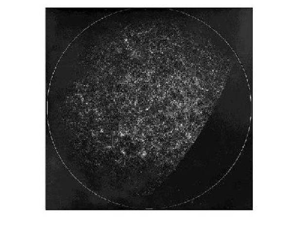
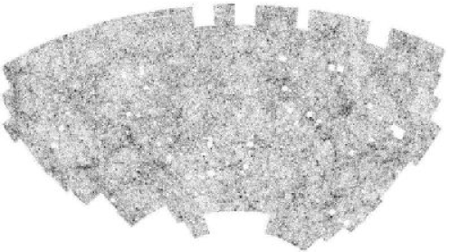
The Cambridge APM survey followed in the early 90’s cataloguing about 2 million galaxies in the Southern Galactic Cap. Maddox et al. 1990. See figure 1.2
Redshift Surveys
Redshift measurements involve determining the spectrum of the object to be measured. Once that is known, recognisable spectral lines can be found, and their deviation from their normal positions used to find the object’s redshift. The Hubble Law then allows one to turn that redshift into a radial distance from our galaxy.
When redshifts were first being measured, it would typically take a few hours on a large telescope to collect enough photons to obtain the required spectrum. Once telescopes with enough light gathering power became available and spectroscopic detectors became sophisticated enough to allow many redshifts to be taken simultaneously in a reasonable amount of time, astronomers started using these instruments to make maps of the 3 dimensional locations of galaxies and galaxy clusters.
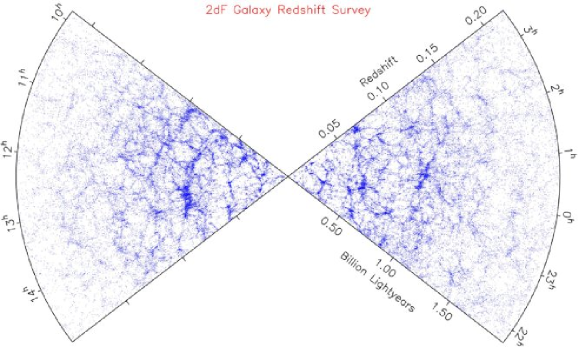
Figure 1.3 is a representation of some of the measured 3 dimensional galaxy positions in redshift space. The radial coordinate in this plot is the measured redshift (essentially indicating the distance from us) and the angular coordinates represent the angular position of the objects in the sky. Thus the 3-D mapping of the universe began:
-
•
In the late 70’s red-shift surveys finally became a reality with the very successful CfA (Center for Astrophysics) survey (Huchra et al. 1983). They managed to record 1100 spectroscopic red-shifts.
-
•
In the early 90’s the PSCz red-shift survey (Saunders et al. 2000) mapped 15,000 spiral galaxies from of the sky. This still stands as the largest survey in terms of sky coverage.
-
•
From 1998 to 2003, the Two Degree Field Galaxy Redshift Survey, using the Anglo-Australian telescope, accumulated 220,000 galaxy red-shifts. See Colless et al. 1999. This survey is illustrated in figure 1.3.
-
•
The Sloan Digital Sky Survey (SDSS) is an ongoing attempt to collect 1 million galaxy red-shifts. The current release, DR5, contains 674,749 galaxies. See Percival et al. 2006 (DR5) and Abazajian et al. 2005 (DR4).
1.3.1 Problems with this view
The information directly available to us on the observed spatial distribution of galaxies is systematically biased compared to the true galaxy distribution.
Angular positions are trivial, but precise distance estimates are more difficult to obtain. More serious, however, is the problem that the sampling rate of observable galaxies depends strongly on redshift. If one considers the universe to be homogeneously distributed with matter, then we would expect the number of objects, in some observed solid angle of the sky, to grow as . However this is not what we actually observe, instead we see distributions like figure (5.5), where the reference curve initially has the form of but soon drops off. This effect is due the diminished flux of faraway objects and our inability to collect enough photons from them to make valid observations. This ‘selection effect’ can be visualised in figure (1.3), as the fall off in the apparent number density of sampled galaxies at larger redshift. This is accounted for by weighting each observed object with the inverse of the selection function, , this increases the contribution of counted objects. The functional form of the selection function is,
| (1.4) |
In the above expression and are set parameters and is the proper distance to the observed galaxy.
Apart from the red-shifts, distances can also be estimated from the flux, , received from a source. To accurately use this method, the intrinsic luminosity, , of the source must be well known and that it radiates in a particular fashion, i.e. beamed or uniform. Considering the source to radiate uniformly, the distance can be calculated from,
| (1.5) |
The main problem with this distance estimator is that the vacuum of space is not so empty. It is filled with dust particles and gas, collectively termed the Interstellar Medium (ISM). The ISM can cause extinction of light (diminished flux) and leads to eq.(1.5) giving the wrong answer. The extinction of light is maximal at low galactic latitudes due to the dust content of our own galaxy. In fact at its worst this effect can completely block out the light coming from distant sources.
In figure 5.4, the masked regions (black) are shown for the PSCz survey. The majority of it is due to the extinction of light through the galaxy. The sweeping arcs (north and south) are due to cryogenic problems in the satellite near the end of the survey period, it was not completed. In figure 4.1, some masked regions for the 2dF survey are shown. These masks are placed over the survey because local object may be blocking the view in a particular direction.
Chapter 2 The Universe at Large
Of the four fundamental forces of nature, the universe on large scales is governed by a single force: Gravity. In the proceeding section we will employ the use of Einstein’s General Relativity to construct the main equations of cosmological evolution. From there we will relax our use of complicated tensor algebra and work in a Newtonian approximation to study the departures from the homogeneous Friedmann equations, due to the growth under gravity of tiny density inhomogeneities in the Universe. This is the ‘first order’ Universe.
2.1 General Relativity
In 1915 Einstein developed the theory of General Relativity to explain gravity as a consequence of the fundamental connection between the geometry and matter content of space-time. This can be summed up in the neat phrase ‘Space-time tells matter how to move and matter tells space-time how to curve’. More specifically, Einstein developed a set of equations which balanced the curvature of space-time and the matter it contained. It is this curvature which generates the force of gravity and determines how matter moves within it. Generally, this can be written as,
| (2.1) |
To explain the ideas and physical motivation of the above equation is beyond the scope of this thesis (for further details see Misner et al. 1973 and Weinberg 1972 for a more physical description). In eq.(2.1), is the Einstein tensor, and are the Ricci tensor and scalar respectively. is the space-time metric and is the Cosmological Constant. Although its inclusion in eq.(2.1) was described by Einstein to be his “Greatest blunder”, it is nowadays a very crucial parameter in cosmology. We will describe in more detail each of the above parameters as we go along.
In our study of cosmology we need a theory of gravity, which we have, and a metric to describe the space-time. A metric is a function that measures the distance between events in space-time. Assuming that the CP is true, the form of this metric must conserve the CP as described in §1.2; i.e. it must be homogeneous and isotropic. To construct the metric with the CP in mind, we slice up the 4-D space-time along hypersurfaces, i.e. constant time.
To impose isotropy it is easier to tackle this problem in spherical coordinates since there is no preferred direction. For homogeneity we insist that the Ricci scalar is constant at all points on the hypersphere. And since we are dealing with a universe which is expanding it would be to our advantage to use a coordinate system which reflects this property. So we will work in a comoving system and therefore preserve the positions of galaxies relative to one another. Under the above assumptions it can then be shown (e.g. Carroll S.M, 2004) that the metric takes the following form,
| (2.2) |
This is known as the Roberson-Walker metric (hereafter RWM). In the above expression is the cosmic scale factor, is a constant which determines the spatial curvature and we are working in units where . may take any real value but by suitable re-scaling of our coordinates it is only necessary to consider 3 possibilities.
-
•
, corresponds to zero curvature and thus a flat universe. Initially parallel trajectories remain parallel.
-
•
, has positive curvature and the universe is closed. Its geometry is like the surface of a sphere. Initially parallel trajectories will converge.
-
•
, has negative curvature and leads to an open universe. Its geometry can be represented by the surface of a saddle. Initially parallel trajectories will diverge.
The RWM in component notation is,
| (2.3) |
With the above information about the metric we can go about obtaining the non-vanishing components of the Christoffel Symbols, . The components are calculated via,
| (2.4) |
where is a summation index and a comma denotes partial derivative. Now it is merely a case of turning the handle to derive the essential non-zero elements of the Christoffel Symbols for the metric given by eq.(2.2),
| (2.5) |
From the above set of equations we can now determine the nonzero components of the Ricci tensor, .This is constructed by contraction of the Riemann tensor, .
| (2.6) |
Summation is implied on the index according to the Einstein summation convention. The components of the Ricci tensor are therefore related to the Christoffel symbols, above by,
| (2.7) |
In the above expression summation is implied over and . As an example this leads to, for the component:
| (2.8) | ||||
The rest of the nonzero components are:
| (2.9) | ||||
The Ricci scalar, , is then obtained via the contraction of i.e,
| (2.10) |
Therefore,
| (2.11) | ||||
Now looking back at equation (2.1), we can compute everything on the RHS of this equation. To evaluate the LHS we must define our energy-momentum tensor, . This tensor describes the matter and energy content of the universe. A perfect fluid approximation is completely defined by two quantities: the rest frame energy density and the isotropic rest frame pressure .
| (2.12) |
Now using eq.(2.12) with eq.(2.1) and assuming that , we can obtain two different equations. From the component we get,
| (2.13) |
and from the other components we obtain
| (2.14) |
These expressions are known as the Friedmann equations. is the Hubble parameter and is defined as,
| (2.15) |
Apart from the global expansion, we can now investigate other aspects of the RWM universe. The density parameter, is defined as,
| (2.16) |
with being the critical density required to produce a flat universe. Combining the above equation with (2.13) gives,
| (2.17) |
and rearranging this gives,
| (2.18) |
The special case of implies that , and since is a fixed constant it must be concluded that for all time.
2.2 Structure Formation
There are two crucial observations that any model of structure formation has to explain: the quadrupole anisotropy of CMB, as measured by WMAP, is one part in 105 (Hinshaw et al. 2003) suggesting that the amplitude of the fluctuations was very small at the epoch of recombination; while redshift surveys of the Local universe show highly inhomogeneous matter distributions over galactic and cluster scales. The gravitational instability is believed to be the physical mechanism which amplifies the small primeval fluctuations into the structure that we observe today.
We now have the main ingredients for analysing the evolution of structure, at least within a linear approximation, these are contained within equations (2.13)-(2.15). Combining the Friedmann equations and rearranging gives us the continuity equation,
| (2.19) |
which shows the conservation of energy as the universe expands. To proceed we will also make the assumption that the matter content of the universe is well described by an ideal gas equation of state, i.e.,
| (2.20) |
In standard cosmology we assume that the majority of the matter is in the form of cold dark matter (CDM), which has the equation of state, . So the pressure component is assumed to be negligible which greatly simplifies the following calculations.
In eq.(2.2) the effect of the curvature is small for distances much less than the Hubble radius (a variety of observations clearly favour and therefore ). Hence, the RWM is well approximated by (similar to the flat Minkowski metric of special relativity but with a time varying rescaling.), where denote the comoving Cartesian coordinates. Assuming a conformal Newtonian gauge111Also known as the longitudinal gauge. This transform is very useful when considering scalar perturbations. (cf. Ma & Bertschinger 1995) the Einstein field equations applied to the first-order perturbations of such a metric yield the Poisson equation of Newtonian gravity:
| (2.21) |
where indicates the fluctuation of the mass density about the mean density and is interpreted as the Newtonian potential. Note that eq.(2.21) does not assume that is small.
2.2.1 The Eulerian Formalism
The Eulerian Formalism considers the large scale universe as a continually expanding fluid, whereby momentum, energy and mass conservations are encapsulated within the equations below:
| (2.22) |
| (2.23) |
| (2.24) |
Equations (2.22)-(2.24) are the equations of motion of a non-relativistic perfect fluid in comoving coordinates. Eq.(2.22) is the continuity equation (expressing mass continuity) and eq. (2.23) is the Euler equation (conservation of the linear momentum). In this system of differential equations the over-density field, , appears rather than the usual density field,
with being the spatially averaged mean density and the peculiar velocity, , is defined as
| (2.25) |
Over-dots indicate partial time derivatives. The pressure is related to the density through equation (2.20). For adiabatic perturbations there are no spatial variations in the equation of state, therefore .
The Linear regime of Adiabatic perturbations
Linearising our system of equation, we obtain
| (2.26) |
| (2.27) |
| (2.28) |
Where represents the adiabatic sound speed, , and the subscript indicates constant entropy throughout the space ().
A general vector field may be decomposed into a (potential) longitudinal and a (rotational) transversal part:
| (2.29) |
From the curl of eq. (2.27) it follows that
| (2.30) |
This implies that rotational modes are not coupled to density perturbations and decay as . Combining the time derivative of the linearised continuity with the divergence of the linearised Euler (cf. eq. 2.27) we yield the equation of motion for the longitudinal density perturbations
| (2.31) |
Since the coefficients are spatially homogeneous (independent of ) this equation may be solved by expanding in plane waves, , , where is the proper wavelength. After some straightforward calculations, it is easy to show that the dynamical behaviour of obeys the following differential equation:
| (2.32) |
where we have defined the comoving Jeans wavenumber by
| (2.33) |
Two qualitative behaviours of the solutions can be easily discerned from eq. (2.32). For wavenumbers larger than pressure dominates the right hand term and perturbations do not grow, merely oscillate. For self-gravity dominates so that gravitational instability can take place. Exact solutions to eq. (2.32) exist for a variety of cases (see, for instance, Peebles 1980). Since the dynamical behaviour of is governed by a second order differential equation, in general, there is one monotonically growing solution and one monotonically decaying solution. In the limit the effects of the pressure are negligible and thus all modes grow at the same rate. In this regime, the general solution to eq. (2.31) is given
| (2.34) |
where and are the growing and decaying modes, respectively, while and are time independent functions (Heath 1977). The decaying solution is a perturbation with initial over-density and peculiar velocity arranged so its initial velocity quickly becomes negligible (Peebles 1980). Thus for most of the history of the universe the growing solution quickly comes to dominate. In an Einstein-de Sitter universe and . For a dust universe with 1, the growing mode is
| (2.35) |
indicates conformal time .
Given a solution for the density perturbation field , the velocity, gravitational potential and gravity field follow. For the longitudinal modes . The gravity field is . Thus, from the system of differential equations, eq’s. (2.26)–(2.28), for , we obtain
| (2.36) |
Where is defined by
| (2.37) |
The behaviour of at the present epoch (=0) is very well described by in the case of universes with negligible space curvature or rather small cosmological constant (Peebles 1980).
2.3 -body Simulations
So far we have only been concerned with the linear regime. To tackle the non-linear regime we must leave our analytical tools behind and instead buy a very big computer to run -body simulations. This is exactly what people have been doing since Sverre Aarseth wrote the first astrophysical -body codes (Aarseth, 1978)222Aarseth helped greatly in the early days of -body simulations by making his codes readily available and easily adaptable..
In the early days of this field, cosmological simulations could only handle roughly 1,000 particles (Goth & Turner, 1979). But with the exponential increase in computing power it was not long until very large -body simulation were being carried out. By the mid-80’s there were 30,000 particles being used (Efstathiou, 1985), this rose steeply to in the 90’s (Bertschinger & Gelb, 1991) and now the most recent effort by the “Virgo Consortium” has seen the first billion particle cosmological simulation (Evrard et al. 2002).
Over the last two decades cosmological -body simulations have played a crucial role in the study of the formation and evolution of cosmic structure. Primarily they have been used to match theory with observations. However, simulations like the recent “millennium run” (Springel et al. 2005) use only dark matter particles which form the gravitational potentials for structure growth. Therefore, there is a crucial step to go from dark matter particles to dark matter halos and finally individual galaxies. The basic technique for doing so is discussed in §5.3.1. One would hope that in this process we are not masking some underlying physics.
The impressive progress achieved in the observational front with the completion of very large surveys such as 2dF and SDSS poses a clear challenge to the numerical work in cosmology: the precision of the predictions provided by the current -body experiments have to be of the order of a few percent.
-body simulations, however, do not include all relevant physics like magnetic fields and gas dynamics. They also have resolution issues, which must play a roll on small scales. So while modern simulations are undoubtedly very useful tools, they must be used with care.
Chapter 3 Quantifying The Large Scale Structure
The issue of quantifying structure is not confined to cosmology, it is a complex matter which stretches across many areas of science. Patterns are there to be identified and exploited in order to find subtle connections and correlations between observables. This method of analysis can be seen in fields as diverse as studying the stock market and modelling biological systems. A wide variety of different statistical tools have been employed to quantify structure, but in studies of the large-scale distribution of galaxies perhaps the most common has been the 2-point correlation function
3.1 The Two Point Correlation Function:
The two point correlation function (hereafter 2PCF), , is defined as the excess probability, with respect to a Poisson distribution, of finding two galaxies in volumes and separated by a distance . The joint probability is then,
| (3.1) |
where is the average density of the sample. This is however not a straight forward working definition since we know that density is varying through the space. Consequently it is not straightforward to identify how large a volume of space must be sampled in order to reliably measure the average density of the galaxy population. Equally importantly, even if such a ‘fair sample’ volume can be identified, the number count of observable galaxies within that volume will not generally be a reliable estimate of the ‘true’ number of galaxies in the volume because of observational selection effects - i.e. a radial selection function and angular masked regions. Also, measuring accurately the distance of galaxies in a survey is not straightforward: redshifts are distorted by peculiar motions and redshift-independent distance indicators (e.g. using some form of ‘standard candle’ assumption) are rather noisy.
For this work we proceed to measure the mean density as the number of galaxies inside the survey, each weighted by the selection function, ; in practice we perform a Monte Carlo over the sample space (see Strauss & Willick, 1995 and references therein). We can also write the conditional probability, , of finding a galaxy in a volume , at a distance from another galaxy,
| (3.2) |
From this equation it is straightforward to see the properties of the function . For , we recover a uniformly random point set, such that the probability of finding a galaxy in volume is simply proportional to . The case of excess clustering is , where we have more galaxies than in the Poisson case. Then there is also the case where . This case corresponds to anti-clustering, and could be relevant e.g. to some models of galaxy formation where the formation of a galaxy may inhibit the formation of other galaxies in its vicinity.
In general the observed is well described by a power law scaling with distance and it is standard practice in the literature to write the 2PCF as,
| (3.3) |
Here is a characteristic scale length usually evaluated when . This description is however an over simplification as the physics of structure formation is richer in complexity than a simple power law.
One great advantage of using this estimator, is that the Fourier Transform of gives the Power Spectra, , of density anisotropies (see §3.1.4). It is also a statistic which is very easy to visualise and very easy to compute. From it is also possible to determine the correlation dimension, , of the discrete point distribution. is calculated via,
| (3.4) |
For a homogeneous distribution in 3-D we would expect . However, at scales around , (Davis-Peebles, 1983), corresponding to a dimensional value, . We will soon see where expression (3.4) comes from when we discuss generalised dimensions in §3.4.
3.1.1 -Correlation Estimators
There are a few different ways to measure , in the literature but the basic computational structure is more or less the same. The main differences between estimators are usually the way in which they deal with ‘edge effects’ and the ‘shot noise’. We are obviously looking for correlations between galaxies so we begin by centering on a galaxy, and proceed to count the number of galaxies within spherical shells of different radii around the central object. This procedure is repeated by centering on all, or a randomly chosen subset of all, the galaxies in the catalogue to obtain a statistical average. The number of galaxies counted in each cell is then normalised by a Poisson term which is related to the mean density. This estimator is written as,
| (3.5) |
| (3.6) |
where are data-data pairs, are data-random pairs and is the number of galaxies. is the selection function and
| (3.7) |
The problem with eq.(3.6) lies within the mean density term. To obtain , the most accurate method should be to sum over all the galaxies while weighting each by the inverse of the selection function. This is calculated as follows,
| (3.8) |
In the last equation, is the volume and the sum is over all galaxies. To reduce the variance associated with , the average can be taken,
| (3.9) |
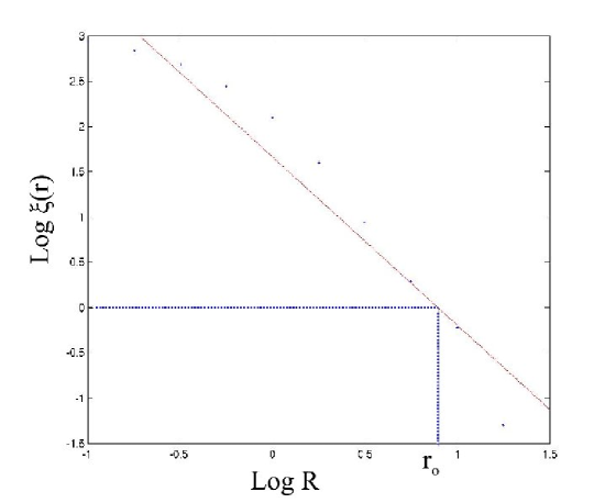
The angled brackets represent a statistical average, which usually invokes the use of the cosmological ergodic theorem (see §3.1.2). The result of applying eq.(3.6) to a mock galaxy catalogue can be seen in figure 3.1. The red line is a straight line fit to the data, giving .
So far we have used and , however pairs are also useful in calculating the 2PCF. Other estimators like the minimum variance estimator, by Landy & Szalay (1993), use the pairs to help correct for boundary effects. Their estimator takes the form,
| (3.10) |
where the is the number of random points. There are many more estimators for the 2PCF. Kerscher, Szapudi, & Szalay (2000) show that equation (3.10) is strongly preferred over other methods.
3.1.2 Ergodicity
A short note on the Ergodic Principle: The observed universe is unique. This implies that averages have to be spatial ones. Such averages will be equal to those obtained if instead we were to average over an ensemble of universes if the Cosmic Ergodic Theorem holds. Ergodicity in the cosmological context means that ensemble averaging and spatial averaging are equivalent. Note that, in contrast with the common practice in statistical mechanics, the cosmological Ergodic Hypothesis refers to the spatial distribution of a random field at a fixed time rather than to the time evolution of the system. Thus, for instance, the ensemble average of the random field at a point , , is simply the expectation value of the random variable .
3.1.3 Gaussianity
Let us introduce some of the statistics used by cosmologists to characterise the spatial distribution of matter. We define r.m.s. fluctuations of a continuous density field as
| (3.11) |
and the correlation function by
| (3.12) |
(Note that for a homogeneous and isotropic random process only depends on the distance between the two points .) The correlation function is a measure of the spatial correlation of the field .
A random field is said to be Gaussian if all -point multivariate probability distribution functions are multivariate Gaussian distributions defined by their mean vector (which the ergodicity implies to be identically zero) and their covariance matrix . Gaussianity is a very popular assumption for two reasons. The first one is that the calculations are “easy” to perform. The second reason is that the CMB seems to support a Gaussian initial density field, Komatsu et al. 2003.
3.1.4 Power spectrum
If we expand the field in plane waves as
| (3.13) |
we see that its Fourier transform is given by
| (3.14) |
where may be thought of a “fair sample” of the universe. The power spectrum of the density field is defined as the expectation of the two-point function in Fourier space, as follows:
| (3.15) |
where is the well-known Dirac delta function. This implies that even if is not a Gaussian distribution, the random variable , being an infinite sum of independent random variables, will still be Gaussian by the Central Limit Theorem for some well-behaved power spectra. We can see that the Dirac function in eq. (3.15) is required because of the translational invariance, . Similarly, we can also see that isotropy implies that depends only the magnitude of the wave-vector .
3.1.5 Window Functions
For some calculations it may be necessary to apply a cutoff at high spatial frequencies, this is due to non-linearities on small scales. The smoothed field that may be obtained by convolution of the “raw” field with some weighting function (called window function) having a characteristic scale is given by
| (3.16) |
has r.m.s. fluctuations given by
| (3.17) |
Where is the representation in Fourier space of . The window function has the following properties: if , if , satisfying the relation . One of the most common window functions is the “top hat” (TH) window function which is defined by the relation
| (3.18) |
where denotes the Heaviside step function if and if ). Another commonly used window function is the Gaussian kernel:
| (3.19) |
3.2 Higher Order Correlations
It is a natural question then to ask whether there are higher order correlations than the simple 2PCF, generally defined as, . The answer is most definitely YES. A Gaussian random field would in principle be completely defined by the 2PCF (the initial density field is thought to have this property), however due to non-linear structure formation we now have local non-gaussianity which means we must look to higher order moments to accurately quantify the galaxy distribution.
These higher order correlations are defined as, , where n is the order of the correlation function. As an example the 3 point correlation function is defined as the joint probability of there being a galaxy in volume elements and given that these elements have displacements and from the galaxy which is being investigated. This is illustrated in fig.(3.2). The joint probability can be written as,
| (3.20) |
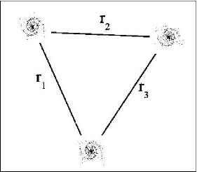
where , and are the sides of the triangle. Assuming homogeneity and isotropy means leads to being a symmetric function of the three lengths. Equation (3.20) is the full three-point correlation function, and is known as the reduced part.
The conditional probability of finding two objects to complete the triangular configuration given that we are centring on a galaxy is,
| (3.21) |
Then the conditional probability of finding a galaxy to complete the triangle, given that we have a pair of galaxies with separation , is,
| (3.22) |
In extending to N-point correlation functions the computational load is increased exponentially. This limits our ability to determine accurately , however there may be a way to avoid this problem by making some approximations.
Given that can be represented by a power law,
| (3.23) |
the 3PCF is then found to be well described by a combination of ’s (Peebles, 1980), i.e.,
| (3.24) |
with (Meiksin, Szapudi & Szalay, 1992).
3.3 Minimal Spanning Trees
One draw back with the 2PCF, as we have defined it in eq.(3.1), is that it is insensitive to filamentary structure. This is due to it being a function only of distance and not direction; thus all angular information is lost through the averaging. The Universe does appear to contain filaments, walls and other such features, but whether these are real or due to chance alignments has of course been a topic of debate over recent decades.
To quantify this kind of structure Barrow, Bhavsar and Sonoda (1985) introduced a method from Graph Theory, called Minimal Spanning Trees (MST). The procedure to implement this is as follows:
-
1
A galaxy A is chosen as a starting point within a 3-D galaxy distribution.
-
2
The nearest galaxy to A is labelled B and a straight line is drawn to connect the two. This line is known as a path.
-
3
The closest galaxy to the set of previous galaxies (in this case A and B) is added to the set and is connected to the closest galaxy in the set. This produces a branching behaviour, and this step is repeated.
-
4
After some time we are left with many paths and circuits (closed paths). If there are no circuits the graph is open and this is known as a tree.
-
5
To then transform this abstract visualisation into a numerical representation of structure we can do a few things, e.g.:
-
i
Calculate the number of lines in angular bins of w.r.t an adjoining line.
-
ii
Calculate the number of lines in distance bins, dr. Obtaining dN vs dr.
-
i
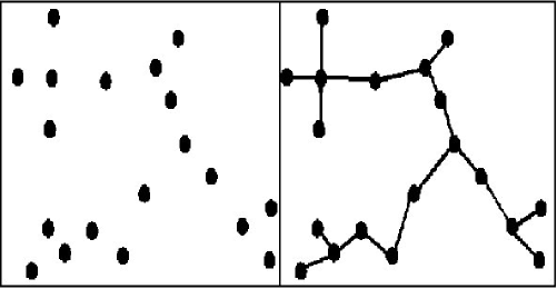
This method connects all galaxies in some fashion. But we know that not all galaxies are physically connected, as a galaxy in one cluster has little to do with another galaxy in a distant cluster.
To account for this, we adjust the previous method by only joining a galaxy to a pre-existing tree if its distance to the closest member is less than some threshold distance. This technique is known as separating and was introduced by Clark & Miller (1966). This method was recently applied to the SDSS DR1 by Doroshkevich et al.(2004). They found that groups and clusters are more likely to be found close to walls rather than filamentary structure.
3.4 The Fractal Universe
Fractal patterns can be thought of as the place where chaos and order meet. This is because self-similarity (fractality) seems to be an eventual by-product of chaotic systems. Fractal pictures are usually associated with “Julia” and “Mandelbrot” sets named after the French mathematicians.
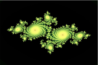
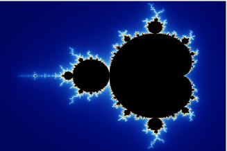
Fractals belong to a branch of mathematics known as Fractal Geometry. Unlike the usual definition of Geometry, where regular shapes and patterns are studied, fractals can be highly irregular and the dimensions which are explored are not confined to integer values like for surfaces and for volumes. The term fractal was originally coined by Mandelbrot himself, who is widely considered the father of fractal studies. In fig.(3.4) the Mandelbrot and Julia sets are shown. These are classical examples of fractal patterns, we can easily see that zooming in on certain areas will yield patterns which are reproductions of the whole picture. It is this self-similarity in fractal patterns which make them scale-invariant objects. Multifractals on the other hand are not scale invariant, since their spatial dimension can vary with scale length. In these terms monofractals can be thought of as a special case of a more general multifractal.
Fractals were merged with the physical sciences through their intimate connection to nonlinear physics and chaotic dynamics. In configuration space we may have chaotic motion for an unstable system, however, in phase space dynamics may be more ordered and the system may evolve towards an attractor. This is rather like a chaotic analogy to an equilibrium state. Phase space trajectories are, however, by no means an easy-to-use tool for analysing structures since, in cosmology, we only have access to spatial coordinates111This is not entirely true as we do have limited velocity information as well.. Nevertheless, this kind of ordered phase space gives rise to a self similar pattern in real space. This is, more specifically, a fractal pattern.
Now it is known that on large scales, the main ingredient to structure formation is the force of gravity. However the potential for gravity leads to highly nonlinear motions and also to cross talking between different spatial scales. So it is not so great a jump to consider the galaxy distribution as a fractal of some kind. In fact this line of analysis is not a new one. The distribution of galaxies in the universe has already been shown to be well described using a multifractal framework, see e.g. Jones et al. 1988.
3.4.1 Multifractal Formalism
In this analysis we will adopt the procedure layed out in Henschel et al. (1983) to determine the Rényi (Generalised) dimensions of a point set embedded in a three-dimensional Euclidean space. The probability of a galaxy, , being within a sphere of radius centred on galaxy is,
| (3.25) | ||||
Here is the number of galaxies within radius , is the total number of galaxies and
| (3.26) |
Equation (3.25) can then be related to the partition sum via Grassberger and Procaccia’s (1983) correlation algorithm,
| (3.27) |
In this case is the number of counting spheres and defines the generalised dimension we are investigating. is the scaling exponent, which is then related to the infinite set of dimensions through,
| (3.28) |
Clearly the special case of , the information dimension, cannot be determined using the above expression but can be found approximately in the limit . This is an important dimension to calculate as it gives equal weighting to voids and clusters. Voids are enhanced for and clusters are enhanced for , so is in this sense the most unbiased dimension in the set. To determine more accurately we must calculate,
| (3.29) |
where is the partition entropy of the point set.
In §3.1 the 2PCF was related to the correlation dimension, , through a differential operation. However, in Multifractal terms the correlation dimension is only one of an infinite number of generalised dimensions which we can use to characterise the distribution. Other important dimensions include, - information dimension, - Capacity dimension, and as . Multifractal distributions are usually defined by a curve which generally decreases with (see figure 3.5). Monofractals on the other hand produce a flat curve.
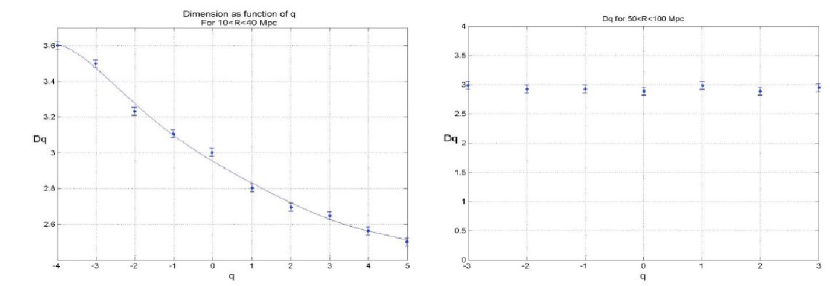
The methodology we have constructed is used to calculate the curve for the CDM -body simulations. The two plots in figure 3.5 show curves for different distance scales. A minimum approach was applied to the partition sum, as illustrated in figure 3.6(a).
The minimisation was performed on a straight line model fit to the data at two different distance scales; Mpc and Mpc. Both and were chosen as they appeared to have constant gradient in these regions. At small scales the data seems to be supporting a multifractal distribution, whereas on large scales the universe appears to reach homogeneity on scales considerably smaller than the size of the box.
3.4.2 Other Estimators
The partition sum can also be calculated using a counts-in-cells approach (Mandelbrot, 1982). Define a new measure of a discrete point set as,
| (3.30) |
which is just the fraction of all galaxies contained within cell . Also if the relation is satisfied, then it must follow that the cells cover the entire space (of topological dimension, ) and that the cubes have volume . We can now construct a new measure,
| (3.31) |
with being the number of occupied cells and is the number of occupied cells, weighted by . The measure is dominated, for large positive values of when the cells are more populated, and for large negative when the cells are sparsely occupied. This is a very important property of multifractal analysis, since under-dense and over-dense regions are probed by different values of .
In the limit , it follows that will be finite and nonzero. Then we can see from eq.(3.31) that,
| (3.32) |
and
| (3.33) |


3.4.3 The Curve
Grassberger et al. (1988) show that we can rewrite the usual fractal measure as,
| (3.34) |
The distribution of the scaling indices characterise the dimensionality of the survey. This is evaluated using the -spectrum,
| (3.35) |
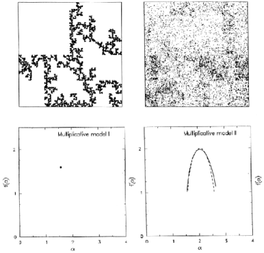
where is the number of times that takes values in the range . For a homogeneous fractal distribution the curve reduces to a single point: In any case the statistical properties of a distribution are equally described by either the generalised dimensions, or by the curve since they are a Legendre pair, as shown below. The only main drawback, as we will soon see, is that the latter strategy requires an extra differentiation of the data.
We can show this by considering the integral version of equation (3.27),
| (3.36) |
A solution to the above expression can be found using the Laplace integral approximation (Martinez et al. 1990), giving,
| (3.37) |
The conditions of this theorem defining the function are,
| (3.38) |
and
| (3.39) |
Using and (3.37) we get,
| (3.40) |
and using (3.38) with (3.39) leads to,
| (3.41) |
Equations (3.40) and (3.41) relate the variable pairs, and : a Legendre transform. So we can see that the distribution is equivalently characterised using either method. However, in practical terms the Generalised Dimension approach may prove to be more accurate, since the curves require a further differentiation of the data. i.e. curves (fig.3.7) are related to the derivative of the ’s (fig.3.5), through eq.(3.41)
In figure 3.7, two realisations of a multiplicative random fractal are shown with their corresponding curves. The method for constructing these distributions is discussed in Jones et al. (1988).
Chapter 4 Boundary Corrections
As we touched on in §1.3.1, the analysis of redshift surveys is prone to many problems, some subtle and some not so subtle. The presence of large ‘holes’ in a survey – regions where no galaxies have been observed – is clearly an example of a serious problem which needs to be appropriately corrected for.
To analyse real (or indeed mock) galaxy surveys we must, therefore, deal with the practical issue of incomplete sky coverage. This can arise firstly because of the geometry of the survey, which is usually a thin beam or a fan. Figure 4.1 illustrates the latter case for the recent example of the 2dF galaxy redshift survey (2dFGRS, Colless et al. 1999). The figure shows the projected distribution of galaxies on the plane of the sky, from which we see that the coverage of the survey is not all-sky – i.e. we do not sample galaxies over steradians. Also, we notice that there are small patches and strips within the geometrical area of the survey which were not sampled.
Secondly, incomplete sky coverage can be caused by the extinction of light through parts of our own galaxy, or regions being obscured by local objects. Hence, for example, even redshift surveys such as the IRAS PSCz (Saunders et al. 2000) which set out to be all-sky are missing galaxies within a ‘mask’ close to the plane of the Milky Way galaxy.
Thirdly, of course, as we already discussed in §1.3.1, redshift surveys are affected by radial incompleteness, which we describe in terms of a selection function, caused by the flux limit below which distance galaxies are too faint to be observed. We can see the influence of this flux limit in Figure 4.1, which shows the variation in magnitude limit from plate to plate in the 2dFGRS.
So, in summary, information about the ‘true’ population of galaxies is hidden or distorted by the effect of a flux limit, by the presence of masked regions and by the boundary of the survey itself.
There has been a number of methods created to account for the problems mentioned above. In the following sections a few of these methods will be reviewed and in §4.6 a new correction technique is introduced, whose benefits include computational and statistical efficiency.

4.1 Deflation Method
As we consider placing spherical shells of increasing radius around a galaxy, even allowing for our ‘weighting’ of the number count of galaxies in each sphere by the radial selection function of the survey, it is clear that we will eventually reach the edge of the survey (which of course we can think of as the distance beyond which the selection function is equal to zero). Therefore, unless some form of edge correction is applied, further increases in the shell radius will result in an estimate of the density for shells that are systematically underpopulated relative to the mean density of the underlying galaxy population, because of the volume of each shell that lies outside the survey. This effect is illustrated in the upper panel of Figure 4.2. For the outer (shaded) shell in this diagram, the estimated density will be systematically lower than the true density since the shell includes a region that lies entirely outside the survey volume and so, by definition, will contain no galaxies.
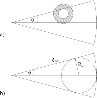
The deflation method is, perhaps, the simplest and crudest form of boundary correction. It simply restricts the sum in equation (3.25) to include only those counting spheres which lie completely within the survey region. However, this drastically reduces the distance out to which the density estimator can reliably probe, leading effectively to a ‘cosmic variance’111Cosmic variance is the cosmologist’s definition of sample variance. If the scales being sampled are comparable in size to the survey, then only a few independent measurements can be taken, i.e. only a few values available for averaging. problem at larger radii.
The maximum scale, which is probed using the deflation method is defined as (Hatton, 1999),
| (4.1) |
where is the opening angle of the survey and the volume limit.
As an example, the Stromlo-APM redshift survey (Loveday et al. 1992) had an opening angle, and a volume limit, Mpc, this leads to a maximum sampling radius of only, Mpc.
4.2 Capacity Correction
The capacity correction can be thought of as the next step up from the deflation method. Here we allow all counting spheres while using equation (3.25), even those which cross the boundary or contain masks. The missing volume is accounted for by re-weighting the contribution of the (incomplete) counting sphere, essentially equivalent to filling it with a distribution of mock galaxies. The main problem is in deciding which distribution should be used to fill the void. Borgani et al. (1994) chose to weight each cell by a factor which is determined by the missing volume.
This at first glance may seem to be a valid choice. On the other hand the weighting factor should be, more correctly, proportional to some measure of the average density in the counting sphere. This highlights the potential problem with the capacity correction: even though it can, in principle, be applied to considerably larger counting spheres than the deflation correction, its form is fundamentally flawed since it is assuming an answer to the question being posed – i.e. that , which is a statement of exactly the homogeneity that we are trying to test.
In practise the capacity correction is applied using the expression,
| (4.2) |
| (4.3) |
to obtain the corrected number of objects within radius from a given particle. The RHS of eq.(4.2) contains two main terms: the reduced number count, , and a term accounting for galaxies which are missing. This is done by calculating the missing volume of the survey and filling it with a density corresponding to the average density of the survey.
To determine the missing volume of the sphere one can place random points within it, or equivalently one can shoot off vectors in random directions from the central point in the sphere, and count how many of these lie within the survey. This approach is known as a Monte Carlo technique. The expression for the missing volume, therefore, requires us to determine two numbers:
-
1.
the number of random vectors emanating from the central galaxy which fall outside the survey
-
2.
the total number of random vectors emanating from the central galaxy.
Of course choosing to fill the missing portion of the counting cell with any presupposed density should be considered bad science. What we would ultimately like to do is fill the missing regions with the right amount of particles. To do this we need information which is hidden from us, behind the mask, but the Cosmological Principle may come to our rescue.
4.3 Angular Correction
In 2002 Pan & Coles, used the the assumption of isotropy222The Isotropy of the universe is a cornerstone of modern cosmology so in this case it is not a bad assumption to make. to infer properties of unknown regions, masks and boundaries, from the well known survey space. Essentially they proposed that you can average over the part of the sphere which is observed and use this average to fill in for the missing regions. Of course this has to be done in an angular fashion, since is assumed not to depend on direction.
Assuming that the universe is statistically the same in all directions, they concluded that the number of galaxies in a given solid angle should be comparable to the number of galaxies in the same solid angle but in a different direction. The average density of galaxies per steradian can then be defined. In order to achieve this, they introduce the weighting factor which has values . The value of the weight determines how much of the counting sphere is missing from the survey, and therefore needs to be accounted for. Then the corrected number of galaxies in a cell is computed from,
| (4.4) |
where is the selection function for a flux limited sample. The weighting factor appears in the above expression to increase the number count accordingly, just as the selection function does.
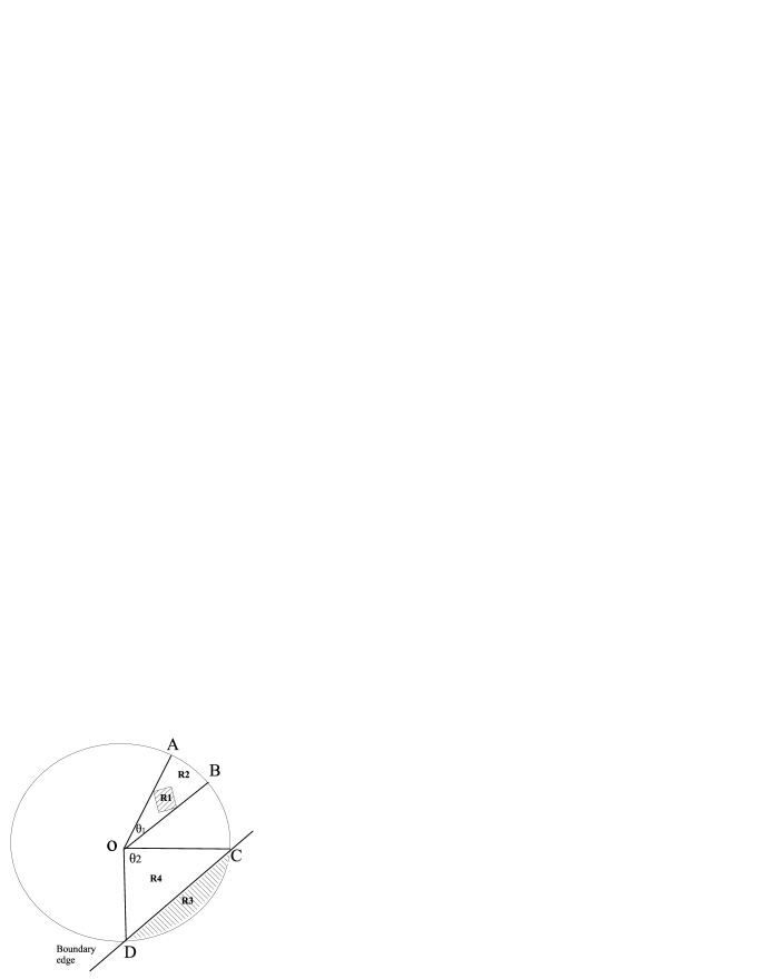
To implement the angular correction one would start as usual and centre on a galaxy within the survey. At a given radius the counting sphere may contain a part of a masked region (indicated by region R1 in fig.4.4) or the survey boundary (R3 in fig.4.4). If this were to occur, the solid angles which contains these features are cut out (slice AOB & COD in fig.4.4) and replaced by an average over the rest of the cell. As an example, for figure 4.4 the weighting factor in this 2-D analogy is . For computational purposes, the method to calculate equation (4.4) is as follows:
-
1
From the set of all galaxies, choose a galaxy as the centre of a counting sphere of radius and determine its position relative to the mask and boundary.
-
2
‘Shoot off’ random vectors () from the centre, where:
-
•
is sampled uniformly . - sphere radius.
-
•
is sampled uniformly .
-
•
, U is sampled uniformly from .
-
•
-
3
Determine which vectors lie outside the survey region. Any vector which does so, save its components.
-
4
Using the scalar product expressed in terms of vector components, calculate the angle between each pair of vectors which lie inside the survey. This allows us to define a reference direction, and a maximum angle, between vectors which lie inside the survey. ( is the opening angle of the cone which points in the reference direction).
-
5
Now begin counting those galaxies in the counting sphere which make an angle, relative to our reference direction.
-
6
The weighting factor, , is then simply related to .
This is essentially the algorithm developed by Pan & Coles (2002) which they tested on simulated catalogues and applied to analyse the fractal clustering of the IRAS PSCz survey.
The angular correction, although in principle a very successful method to correct for boundary effects, is very slow and inefficient. Moreover, and worse still, it throws away potentially useful data. We can see this from Figure 4.4, where the galaxies in regions R2 and R4 are excluded by the angular correction.
In the next section we consider a method which has the potential to improve further upon the angular correction.
4.4 Volume Correction
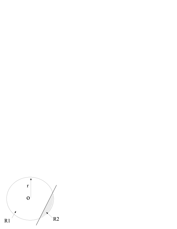
The basic idea of our new, volume, correction can be illustrated in figure 4.3. Here the counting sphere has exceeded the geometrical boundary of the survey. The number of galaxies counted in the sphere of radius is depleted which leads to being reduced through equation (3.25). As we have seen, to solve this problem we could either add galaxies to the missing region, as is the case with the capacity correction, or or equivalently we could somehow modify our definition of the volume itself (hence the name for our new correction!). Of course you may notice that eq.(3.25) does not contain any explicit reference to the volume, but we can cast this equation as,
| (4.5) | ||||
| (4.6) |
with being the true volume of the sphere and being what we can term the reduced volume. We have also introduced the reduced density, , as an intermediary step which need not be calculated, and related this with a reduced volume and number count, . On its own this method can be visualised in figure (4.3), as assigning to the missing region (R2) the same density as that of region (R1). This would be wrong if density varies with distance, so that . To overcome this problem we assume only that the density does not vary with or i.e. the universe is isotropic and hence equation (4.6) will hold for fixed . So to apply this method to a galaxy survey we must count in spherical shells, correcting our estimate of the density in each shell as we go along, and then integrate up the shells at the end. This method is illustrated in figure (4.5). The shells are individually corrected and summed according to,
| (4.7) |
where ; this is the enhancement factor of the shell at radius and has value 1.

The main advantage of this method is that makes the maximum use of the data. Specifically, if the boundary edge cuts across a counting sphere at a particular radius, the method still makes full use of galaxies at smaller radii from the centre of the counting sphere, even if they lie in the solid angle subtended by the boundary edge.
The deflation method and the angular correction, of Pan & Coles, on the other hand throw away a lot of potentially useful data, which limits the counting sphere radius within which the density may be reliably estimated.
4.5 Practical Computing Issues
One significant drawback faced when implementing the angular correction is that it must fill the counting spheres with random vectors to determine the missing regions. To obtain the required resolution means placing many random vectors at the centre of the sphere. For a cell with we have found that this requires the generation of random points.This is not a trivial computational task given that the vectors must be computed and angles stored at every step.
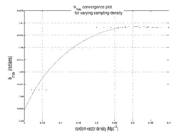
To see where this comes from consider figure 4.6. Here a simulation has been set up to mimic what happens when computing the angular correction. A counting sphere is placed close to the survey boundary and is calculated for varying numbers of random vectors. From the plot we can see the convergence of the opening angle at an approximate vector density of . Taking this value we can make a back of the envelope calculation of the required number of random vectors to accurately constrain at a typical scale of Mpc. The number of vectors required is then,
To make the comparison with the new volume correction, the same calculation is performed. In this case however we are calculating the number of vectors required to populate a spherical shell with thickness Mpc, as a typical value.
The volume correction is definitely more computationally efficient, especially when you consider that the missing volume must be calculated for every galaxy and at every distance iteration. One should also bear in mind however that these codes could be used on much bigger surveys, SDSS is now pushing 1 million galaxies.
4.6 Error Analysis
Error estimation in fractal analysis has been largely swept under the carpet by many in this field. One of the reasons for this is the computational costs of using, e.g., a set of mock galaxy catalogues to estimate error estimates via a Monte Carlo approach. Nevertheless, we can obtain an approximate expression for the error on an estimate of the galaxy number density via some remarkably simple mathematics.
We follow Grassberger and Procaccia’s (1983) suggestion and use the partition function ,
| (4.8) |
to estimate the generalised dimensions of a set of galaxies. Here is the probability,
| (4.9) |
of a cell, centred on the galaxy, having an occupation number . is the cell size while is a scaling exponent.
| (4.10) |
By construction the mean of the partition function is positive as there are always cells with galaxies within. However, there is a subtlety when handling astronomical data: in expression (4.8) we assume that any set contains an infinite number of elements and the size of the cells vanish. Redshift surveys, however, contain a finite number of objects in a finite volume. This will lead to configurations where none of the cells have galaxies other than the central one when .
We can then construct the second moment of the distribution and rearrange as below,
| (4.11) | |||
| (4.12) | |||
| (4.13) | |||
| (4.14) |
| (4.15) |
Where represents an ensemble average. Applying the Cosmological Ergodic Theorem to the above equation leads to sums over the cells.
Thus, for the can be cast as
| (4.16) | |||||
| (4.17) | |||||
| (4.18) | |||||
| (4.19) |
We can then estimate the standard deviation directly from,
| (4.20) |
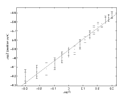
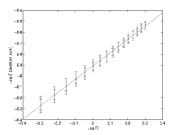
We show a comparison between our error estimation, from eq.(4.20), and an error estimation from 100 simulated Lévy Flight fractals (see figure 4.7).
The left hand plot, of figure (4.7), shows the partition function calculated as a function of distance. To each point is attached a larger error bar estimated from the prescription discussed in §4.6 and a smaller error bar obtained via an average over the 100 simulations. We can see from the plot that the gradient of is constant and the points are all very close to the fitted straight line. The fit was obtained by minimising the function. The right hand plot shows similar points but now the partition function calculated at each distance is also averaged over the 100 simulations, with error bars computed as before. The excellent agreement in the fitted slopes of the left and right hand plots indicates that the partition function is an unbiased estimator.
Chapter 5 Analysis & Results
We will begin in the proceeding section by applying the different corrections to a toy fractal model. This model can be used to compare and contrast the differing methods. Then the volume correction will be used to analyse in detail the distribution of particles produced from an -body simulation.
5.1 The Lévy Flight
An initial test for the different corrections is to analyse a simple fractal distribution, the Lévy Flight. This fractal is very easy to construct and has an analytical determined dimension (see Meakin 1998).
The Lévy flight fractal is finding its way into many areas of physics due to its close connection to Brownian Random Motion. For example it has been used to explain Interstellar scintillation (Boldyrev & Gwinn 2003) and even modelling the financial market (Chowdhury & Stauffer 1999) The Lévy Flight is constructed as follows:
-
1
A point A is chosen at random, maybe the origin, in Cartesian space.
-
2
A displacement is given to A by a vector (,,) to give a second point B. The angular direction is uniformly sampled and the Probability of exceeding a value r is given by,
(5.1) -
3
This procedure is repeated many times to ‘fill’ the 3-D space, which was restricted to a cubic box of side 400 Mpc.
In expression (5.1), is the fractal dimension and is a characteristic scale length, both of which we can adjusted to produce different features. The resulting distribution is not so dissimilar to a true galaxy survey (cf. figure 5.1). can be related to the average inter-cluster separation.
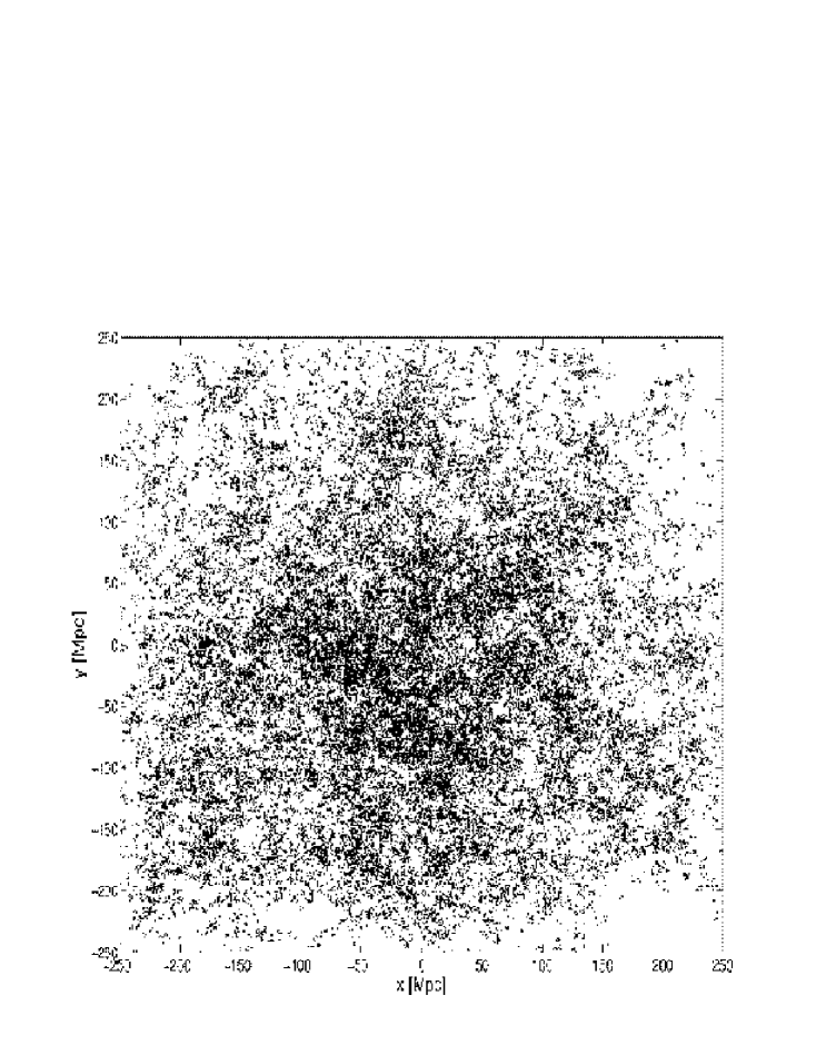
5.1.1 Multifractal Analysis
A multifractal analysis, as described in § 3.4.1, is performed on a Lévy Flight distribution of particles (cf. fig 5.1). The boundary is corrected by considering each of the different methods from Ch.4. This setup should give a fair comparison of the different correction methods.
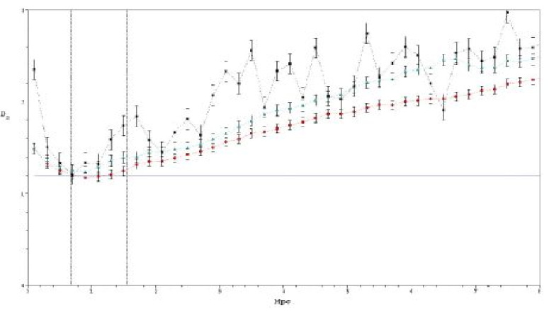
Since the correlation dimension is known analytically, the multifractal analysis will be restricted to the dimension. Now from the partition sum , equation (3.28) will provide the value through differentiation. This differentiation was performed directly on the data by applying a linear fit to every three consecutive data points. The errors, as described in § 4.6, were considered when minimising the function.
The results of this procedure are plotted in figure 5.2. There are a few points to note in this plot. Firstly, the Lévy Flight is highly anisotropic, which is a cause for concern when applying a statistic which does not consider angular information. Although this may be a problem, following the suggestion of Martínez et al. (1990), the correct result from the simulation seems to be confined to the range between the average nearest neighbour separation and the mean inter-particle spacing. In figure 5.2 it can be easily seen that the volume correction lies closer to the analytical answer of , than either the capacity or angular corrections.
Secondly, the volume correction is more or less always closer to the true value, even as the methods begin to over estimate on larger scales. This over estimation by all the methods is due to the anisotropic nature of the Lévy Flight distribution.
Thirdly, the large errors and visual noisiness of the angular correction are not present in either the capacity or volume corrections. This, I can only conclude, is due to the angular method throwing away data, leading to low number statistics, i.e. intrinsic noise.
5.2 CDM Simulation
In this section we will analyse the distribution of dark matter halos from a CDM simulation. Since there are no galaxies in this analysis, it is only the underlying dark matter distribution which is being probed. This simulation was performed by Warren et al. (2006), see reference for a detailed description. For this work we are using a 384Mpc box with a flat geometry and cosmological parameters,
| (5.2) |
Initial conditions were derived from the transfer functions as calculated by CMBFAST (Seljak & Zaldarriaga, 1996). The final catalogue has approximately 1.5 million halo positions.
5.2.1 Multifractal Analysis
The multifractal analysis as presented in §3.4.1, must be applied over a range of different distance scales. In figure (3.5) the results of this analysis are shown over two different ranges; Mpc and Mpc. These scales were chosen almost arbitrarily111The only reason was that the partition sum, , seemed to have a constant gradient in these regions.. The left hand plot of fig.(3.5) shows a clear sign of multifractality on small scales whereas the right hand plot appears to signal a transition to homogeneity. However, since the partition function (like figure 3.6 (a)) is generally smooth, we can expect a smooth transition to homogeneity.
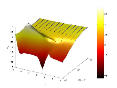
Instead of applying this analysis in certain ranges, the plots in figure 3.5 could be extended by adding another axis: distance. This would give us a Surface.
The Surface
Figure 5.3 shows the result of extending the multifractal analysis to include varying scales. The high peak and dip on low scales (Mpc) corresponds to a multifractal distribution. The surface then levels off to a constant value of three advocating a transition to homogeneity at a scale of Mpc. Another interesting feature is that homogeneity is not reached at the same scale for all .
5.3 PSCz Mock Catalogue
In the previous section the whole halo catalogue was used, thus the analysis is only relevant for the underlying dark matter distribution. In this section the galaxies are under investigation. The galaxy mock catalogue is extracted from the -body simulation (cf. § 5.3.1).
5.3.1 Making Mock Catalogues
Mock PSCz catalogues have been extracted from the -body simulations performed by Cole et al. (1997). They used the AP3M code of Couchman (1991) loaded with 1923 particles in a box of comoving size of 345.6. The particle mass is 1.6210. Further details can be found in Cole et al. (1997). For the analysis performed in § 5 we have considered two different cosmologies (cf. Table 5.1): a flat model and cosmological constant term, and a critical density universe () with power spectrum shape parameter, . The relevant details of the two cosmological models explored are summarised in the table below.
| Model | ||||
|---|---|---|---|---|
| LCDM | 0.3 | 0.7 | 0.25 | 1.13 |
| SCDMG | 1.0 | 0.0 | 0.25 | 0.55 |
Ten different mock catalogues, which we will refer to as LCDM0, SCDMG0, , have been extracted from each of the above models.
Although in this work we have not created an -body code or extracted the mock catalogues from it, it is still worth discussing the procedure for doing so.
-
•
A population of particles with properties similar to those of the Local Group (LG) is identified. A LG-like observer is defined by implementing two observationally based constraints: the peculiar velocity of the point must be km s-1, and the particle must be located in a region for which the fractional overdensity averaged in a radius of 5 is in the range .
-
•
A sphere of 120 radius is drawn around the LG-like observer and the whole frame is rotated so that the motion of the observer is in the direction (, ), the direction of the LG peculiar velocity with respect to the CMB frame (e.g. Wilkinson 1988).
-
•
A friends-of-friends algorithm is implemented to find galaxy clusters. (see Frenk et al. 1988 for details)
-
•
The number density of particles in the simulation is Mpc-3 while the number density given by the PSCz selection function exceeds this density closer than some critical distance. Thus, the simulations are volume-limited for distances less than 10.9, where the PSCz number density (Saunders et al. 1999) matches the -body one. For distances greater than this the simulated surveys follow the PSCz number density.
-
•
A Monte Carlo rejection was used to choose particles according to the PSCz selection function (Saunders et al. 2000):
(5.3) The optimal parameters are listed in Table 5.2. For the mock catalogues are volume-limited and thus . A random flux consistent with the PSCz selection function is then attributed at each selected galaxy.
0.53 1.90 10.90 86.40 Table 5.2: Selection Function Parameters for Eq. (5.3) -
•
Despite the large sky coverage, PSCz is not a full-sky catalogue. Unsurveyed regions are present both at high and low galactic latitudes that need to be accounted for to properly reproduce the existing observational biases. All the galaxies which fall within masked regions have been rejected leaving the final sky coverage to be complete.
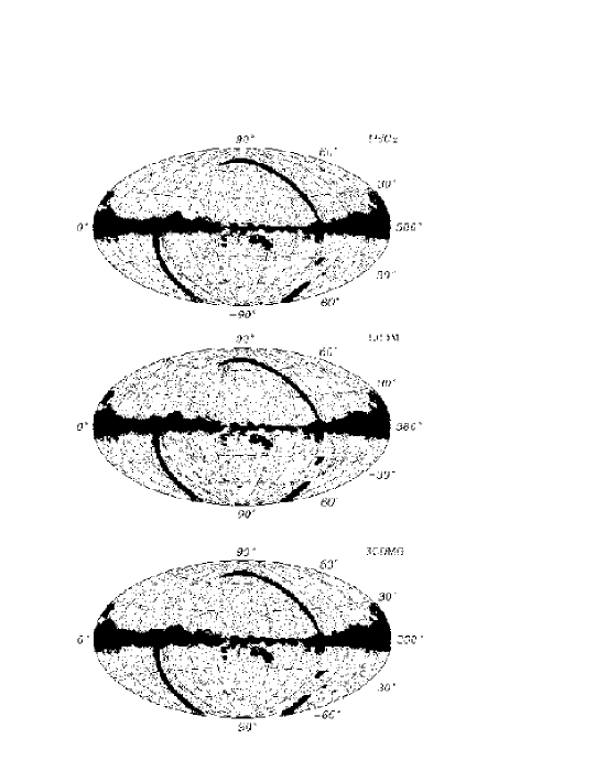
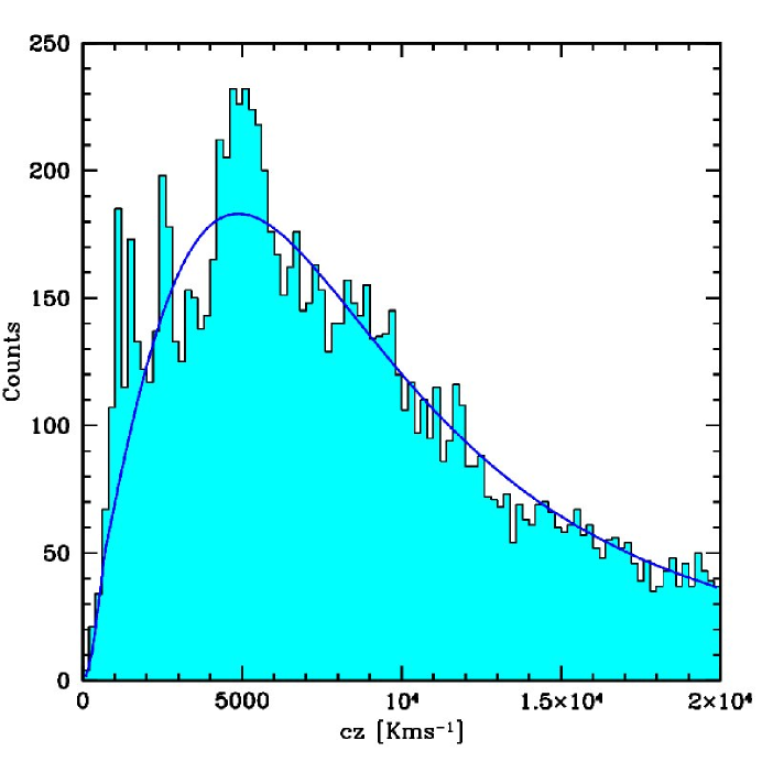
The final mock catalogue contains the positions of the galaxies in redshift-space and their “observed” flux. The galaxy redshifts are assigned by adding the line-of-sight component of the peculiar velocity to the recession velocity.
5.3.2 Multifractal Analysis
Figure 5.3 shows the surface for the halo positions in an ideal and complete box. It has a standard CDM cosmology with no galaxies, so only the underlying dark matter distribution was investigated. Overall, it is a very smooth surface, which tends towards homogeneity at scales Mpc. A clear peak, at low , and dip, at high corresponds to multifractality for Mpc.
The same surface analysis is repeated, this time for the Mock galaxy catalogues mentioned above. The main difference is, now there are a lot less particles to analyse, . However, given that we have 10 mock realisations to average over, the noise should not be much worse. Figure 5.6 shows the averaged surfaces of the CDM and the SCDMG cosmologies.
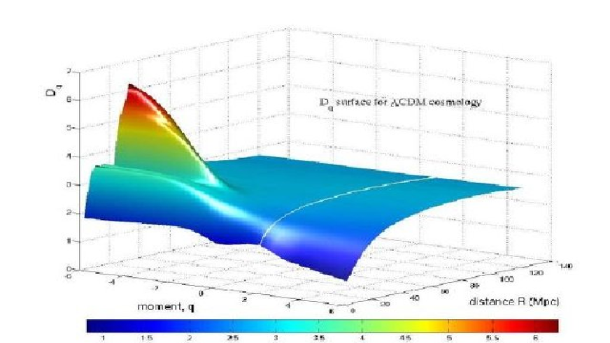
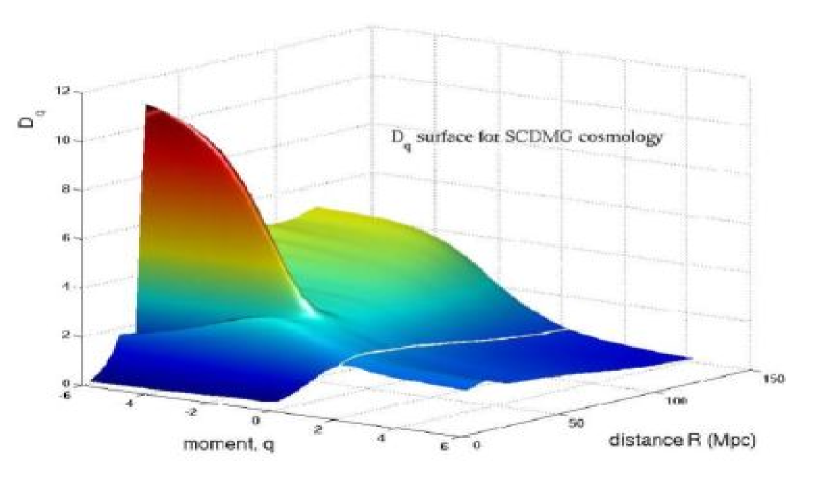
Surface - CDM
There are some points we should note regarding the surfaces of figure 5.6. The CDM cosmology yields a plot quite similar to that of figure 5.3, this should not be too surprising given that they have the same cosmological parameters. There is however clearly a few features on small scale where the two differ. In fig.(5.6) at Mpc there is a multifractal feature peaking at . A little further out at Mpc there is a second multifractal signature with a much higher peak . Recalling that figure 5.6 is an average taken over 10 realisations, it is interesting that the two multifractal features on small scales have not merged into one i.e. they are probably not statistical anomalies. It would be premature to suggest that these distinct features have any physical significance222This same point has been made by Bernard Jones in many of his papers, most recently in the review article (Jones et al. ,2005). but there is definitely room here for further study.
On scales larger than Mpc the surface flattens to homogeneity, . The white reference line shows the correlation dimension, , varying with scale. This is related to the derivative of the 2PCF. Visually this shows that all the information which the 2PCF can provide is but a very small part of the surface.
Surface - SCDMG
In the lower panel of figure 5.6, the surface is plotted for the SCDMG cosmology. It clearly shows on small scales a similar multifractal peak to that of the CDM model. However, there seems to be only one very sharp distinct peak at Mpc and for , . Casting our mind back to §3.4.1, this is telling us that on scales Mpc void under-dense regions are more clustered.
Looking beyond the first peak it can be seen that the surface does not flatten off like the CDM model. In fact on scales beyond Mpc there is no transition to homogeneity in this universe, on scales up to the size of the simulation it is entirely multifractal.
It is evident, therefore, that on large scale the surface can in principle discriminate between different cosmological models.
Chapter 6 Summary
We have shown that our volume correction recovers the true fractal dimension, when tested with the extreme case of an anisotropic Lévy Flight. The increase in accuracy over Pan & Coles angular correction estimator is marginal, however the computational load required is much less. This fact will become increasingly more important as red-shift surveys are now pushing 1,000,000+ galaxies.
We present the surface as a possible unique descriptor of a discrete point distribution. Whether this is strictly true or not does not differ from the fact that there is much more information contained in our multifractal analysis than can be extracted from the usual 2PCF. In fact to go from a 2PCF to our multifractal measure, is of no significant computational cost.
The 2PCF in our formalism, is represented by the integral along the line in figures (5.6) & (5.3). It is clearly apparent that is confined to a rather boring and flat part of the surface and generally for the surface is very smooth and tends towards a constant value without any interesting features.
There has been a lot of interest, since the dawn of cosmological simulations, to apply statistics to the resulting distributions so that a comparison can be made with real surveys. Much of this effort has involved the 2PCF (also Minimal Spanning Trees and other geometrically motivated descriptors). However it must be made clear that the trade off between statistical robustness and visual interpretation is of prime importance when quantifying structure. Neither should be favoured too heavily.
As we have presented here, our surface gives varying weights to under dense (void) regions and over dense (clustered) regions, this obviously has a significant advantage over calculating higher order correlations. The major task now, regarding the surface, is to make full use of it and to extracted as much information as is statistically possible.
Our methodology as presented in §3.4.1 also has the possibility to contribute to parameter estimation. Especially in the area of Baryon Acoustic Oscillations (BAO). BAO’s are difficult to measure accurately due to the low amplitude on scale above 100Mpc. To help increase the power in this range, clusters, instead of individual galaxies, could be used as they show a higher clustering amplitude. This technique has some drawbacks The biggest problem it faces is in accurately determining what is a cluster. Another technique for measuring BAO’s would be to use the surface as we introduced in §5.2.1. Since this method treats dense and under-dense regions differently, it suggests that the usual 2PCF (or ) may not be the best suited to observing and measuring BAO’s. In future work we hope to explore the use of the surface as a cosmological tool.
Bibliography
- [1] S. J. Aarseth. Computer simulations of galaxy clustering. In M. S. Longair and J. Einasto, editors, IAU Symp. 79: Large Scale Structures in the Universe, pages 189–194, 1978.
- [2] K. Abazajian et al.. The Third Data Release of the Sloan Digital Sky Survey. Astro. J., 129, March 2005.
- [3] G. O. Abell. The Distribution of Rich Clusters of Galaxies. ApJ Suppl., 3(211), May 1958.
- [4] J. D. Barrow, S. P. Bhavsar, and D. H. Sonoda. Minimal spanning trees, filaments and galaxy clustering. MNRAS, 216:17–35, September 1985.
- [5] E. Bertschinger and J. M. Gelb. Cosmological N-body simulations. Computers in Physics, 5:164–175, April 1991.
- [6] S. Boldyrev and C. R. Gwinn. Lévy Model for Interstellar Scintillations. Physical Review Letters, 91(13):131101, September 2003.
- [7] S. Borgani, V. J. Martinez, M. A. Perez, and R. Valdarnini. Is there any scaling in the cluster distribution? ApJ, 435, November 1994.
- [8] S. M. Carroll. Spacetime and geometry. An introduction to general relativity. Spacetime and geometry / San Francisco, CA, USA: Addison Wesley, ISBN 0-8053-8732-3, 2004, 2004.
- [9] D. Chowdhury and D. Stauffer. A generalized spin model of financial markets. Euro. Phys Journal B, 8:477, 1999.
- [10] R. Clark and W.F. Miller. Math. Comp. Phy, 1966.
- [11] S. Cole, D. H. Weinberg, C. S. Frenk, and B. Ratra. Large-scale structure in COBE-normalized cold dark matter cosmogonies. MNRAS, 289, July 1997.
- [12] M. Colless. First results from the 2dF Galaxy Redshift Survey. In G. Efstathiou, editor, Large-Scale Structure in the Universe, 1999.
- [13] H. M. P. Couchman. Mesh-refined P3M - A fast adaptive N-body algorithm. ApJ Lett., 368, February 1991.
- [14] M. Davis and P. J. E. Peebles. A survey of galaxy redshifts. V - The two-point position and velocity correlations. ApJ, 267:465–482, April 1983.
- [15] A. Doroshkevich, D. L. Tucker, S. Allam, and M. J. Way. Large scale structure in the SDSS galaxy survey. A&AP, 418:7–23, April 2004.
- [16] G. Efstathiou, M. Davis, S. D. M. White, and C. S. Frenk. Numerical techniques for large cosmological N-body simulations. ApJ Suppl., 57:241–260, February 1985.
- [17] C. S. Frenk, S. D. M. White, M. Davis, and G. Efstathiou. The formation of dark halos in a universe dominated by cold dark matter. ApJ, 327, April 1988.
- [18] J. R. Gott, III and E. L. Turner. An extension of the galaxy covariance function to small scales. ApJ Lett., 232:L79–L81, September 1979.
- [19] P. Grassberger and I. Procaccia. Estimation of the Kolmogorov entropy from a chaotic signal. Phys. Rev. A, 28, October 1983.
- [20] S. Hatton. Approaching a homogeneous galaxy distribution: results from the Stromlo-APM redshift survey. MNRAS, 310:1128–1136, December 1999.
- [21] D. J. Heath. The growth of density perturbations in zero pressure Friedmann-Lemaitre universes. MNRAS, 179:351–358, May 1977.
- [22] H. G. E. Hentschel and I. Procaccia. Fractal nature of turbulence as manifested in turbulent diffusion. Phys. Rev. A, February 1983.
- [23] G. Hinshaw, D. N. Spergel, L. Verde, R. S. Hill, S. S. Meyer, C. Barnes, C. L. Bennett, M. Halpern, N. Jarosik, A. Kogut, E. Komatsu, M. Limon, L. Page, G. S. Tucker, J. L. Weiland, E. Wollack, and E. L. Wright. First-Year Wilkinson Microwave Anisotropy Probe (WMAP) Observations: The Angular Power Spectrum. ApJ Suppl., 148:135–159, September 2003.
- [24] J. Huchra, M. Davis, D. Latham, and J. Tonry. A survey of galaxy redshifts. IV - The data. ApJ Suppl., 52, June 1983.
- [25] B. J. Jones, V. J. Martínez, E. Saar, and V. Trimble. Scaling laws in the distribution of galaxies. Reviews of Modern Physics, 76:1211–1266, February 2005.
- [26] B. J. T. Jones, V. J. Martinez, E. Saar, and J. Einasto. Multifractal description of the large-scale structure of the universe. ApJ Lett., 332, September 1988.
- [27] M. Kerscher, I. Szapudi, and A. S. Szalay. A Comparison of Estimators for the Two-Point Correlation Function. ApJ Lett., 535:L13–L16, May 2000.
- [28] E. Komatsu, A. Kogut, M. R. Nolta, C. L. Bennett, M. Halpern, G. Hinshaw, N. Jarosik, M. Limon, S. S. Meyer, L. Page, D. N. Spergel, G. S. Tucker, L. Verde, E. Wollack, and E. L. Wright. First-Year Wilkinson Microwave Anisotropy Probe (WMAP) Observations: Tests of Gaussianity. ApJ Suppl., 148, September 2003.
- [29] S. D. Landy and A. S. Szalay. Bias and variance of angular correlation functions. ApJ, 412:64–71, July 1993.
- [30] J. Loveday, B. A. Peterson, G. Efstathiou, and S. J. Maddox. The Stromlo-APM Redshift Survey. I - The luminosity function and space density of galaxies. ApJ, 390, May 1992.
- [31] C.-P. Ma and E. Bertschinger. Cosmological Perturbation Theory in the Synchronous and Conformal Newtonian Gauges. ApJ, 455, December 1995.
- [32] S. J. Maddox, G. Efstathiou, W. J. Sutherland, and J. Loveday. The APM galaxy survey. I - APM measurements and star-galaxy separation. MNRAS, 243:692–712, April 1990.
- [33] B. B. Mandelbrot. The Fractal Geometry of Nature. The Fractal Geometry of Nature, San Francisco: Freeman, 1982, 1982.
- [34] V. J. Martinez, B. J. T. Jones, R. Dominguez-Tenreiro, and R. van de Weygaert. Clustering paradigms and multifractal measures. ApJ, 357:50–61, July 1990.
- [35] P. Meakin. Fractal, scaling and growth far from equilibrium. Cambridge University Press, 1998.
- [36] A. Meiksin, I. Szapudi, and A. Szalay. Higher order correlations of IRAS galaxies. ApJ, 394:87–90, July 1992.
- [37] C. W. Misner, K. S. Thorne, and J. A. Wheeler. Gravitation. San Francisco: W.H. Freeman and Co., 1973, 1973.
- [38] J. Pan and P. Coles. Large-scale cosmic homogeneity from a multifractal analysis of the PSCz catalogue. MNRAS, 318:L51–L54, November 2000.
- [39] J. Pan and P. Coles. Boundary corrections in fractal analysis of galaxy surveys. MNRAS, March 2002.
- [40] P. J. E. Peebles. The large-scale structure of the universe. Princeton University Press, 1980. 435 p., 1980.
- [41] P. J. E. Peebles. Principles of physical cosmology. Princeton University Press, 1993.
- [42] W. J. Percival et al. . The shape of the SDSS DR5 galaxy power spectrum. ArXiv Astrophysics e-prints, August 2006.
- [43] W. C. Saslaw. The Distribution of the Galaxies. The Distribution of the Galaxies. ISBN 0521394260. Cambridge University Press, October 1999.
- [44] W. Saunders, S. Oliver, O. Keeble, M. Rowan-Robinson, S. Maddox, R. McMahon, G. Efstathiou, W. Sutherland, H. Tadros, S. D. M. White, and C. S. Frenk. The IRAS Point Source Catalog Redshift (PSCz) Survey. In ASP Conf. Ser., 2000.
- [45] U. Seljak and M. Zaldarriaga. A Line-of-Sight Integration Approach to Cosmic Microwave Background Anisotropies. ApJ, 469, October 1996.
- [46] V. Springel, S. D. M. White, A. Jenkins, C. S. Frenk, N. Yoshida, L. Gao, J. Navarro, R. Thacker, D. Croton, J. Helly, J. A. Peacock, S. Cole, P. Thomas, H. Couchman, A. Evrard, J. Colberg, and F. Pearce. Simulations of the formation, evolution and clustering of galaxies and quasars. nature, 435, June 2005.
- [47] M. A. Strauss and J. A. Willick. The density and peculiar velocity fields of nearby galaxies. Phys. Rep., 261:271–431, 1995.
- [48] W. N. Venables and B. D. Ripley. Modern Applied Statistics with S-PLUS. Springer, New York, 1999.
- [49] J.-M. Virey, P. Taxil, A. Tilquin, A. Ealet, C. Tao, and D. Fouchez. Determination of the deceleration parameter from supernovae data. Phys. Rev. D, 72(6):061302, September 2005.
- [50] M. S. Warren, K. Abazajian, D. E. Holz, and L. Teodoro. Precision Determination of the Mass Function of Dark Matter Halos. ApJ, 646, August 2006.
- [51] S. Weinberg. Gravitation and Cosmology: Principles and Applications of the General Theory of Relativity. ISBN 0-471-92567-5. Wiley-VCH, July 1972.
- [52] D. T. Wilkinson. Recent Measurements of the Cosmic Microwave Radiation. In J. Audouze, M.-C. Pelletan, and S. Szalay, editors, IAU Symp. 130: Large Scale Structures of the Universe, 1988.
- [53] F. Zwicky et al.. Catalogue of Galaxies and of Clusters of Galaxies. vol. 6. In California Inst. Techn., 1968.