The exact numerical treatment of inflationary models
Abstract
The precision reached by the recent CMB measurements gives new insights into the shape of the primordial power spectra of the cosmological perturbations. In the context of inflationary cosmology, this implies that the CMB data are now sensitive to the form of the inflaton potential. Most of the current approaches devoted to the derivation of the inflationary primordial power spectra, or to the inflaton potential reconstruction problem, rely on approximate analytical treatments that may break down for exotic models. In this article, we numerically solve the inflationary evolution of both the background and all the perturbed quantities to extract the primordial power spectra exactly. Such a method solely relies on General Relativity and linear perturbation theory. More than providing a tool to test analytical approximations, one may consider, without complications, the treatment of non-standard inflationary models as those involving several fields, eventually non-minimally coupled to gravity.
The usefulness of the exact numerical approach to deal with CMB data is illustrated by analysing the WMAP third year data in the context of single field models. For this purpose, we introduce a new inflationary related parameter encoding the basic properties of the reheating era. This reheating parameter has significant observable effects and provides a self-consistency test of inflationary models. As a working example, the marginalised probability distributions of the reheating and potential parameters associated with the small field models are presented.
1 Motivations
The inflationary paradigm is currently passing all the tests raised by the so-called high precision cosmology measurements Spergel:2006hy . Although this suggests that the existence of a quasi-exponential accelerated era in the early universe may be viewed as a standard lore, one has to keep in mind that almost all the inflationary field models lasting more than sixty efolds and leading to an almost scale-invariant power spectrum for adiabatic scalar perturbations may do the job. It is therefore of both theoretical and observational interest to look for inflationary properties that are, or will be in a foreseeable future, significant enough in the data to allow disambiguation between the different models. Many works are devoted to this task ranging from the details of the reheating era to the search of a theoretical embedding of inflation in supersymmetry or string theory Bassett:2005xm ; Allahverdi:2006iq ; Allahverdi:2006we ; Tye:2006uv . In the following, we will be interested in the model disambiguation problem through the cosmological perturbations and the Cosmic Microwave Background (CMB) anisotropies.
Among the analytical tools available to study inflation in the cosmological context, the so-called slow-roll approximation provides analytical expressions for both the field evolution and the primordial scalar and tensor power spectra. It relies on an order by order expansion in terms of the so-called Hubble-flow functions , where is the number of efolding from the beginning of inflation and the Friedman-Lemaître-Robertson-Walker (FLRW) scale factor Schwarz:2001vv . The Hubble flow fonctions are defined from the Hubble parameter by
| (1) |
If the underlying field model is such that these functions remain small at the time where the length scales of cosmological interest today leave the Hubble radius, then the scalar and tensor power spectra can be Taylor expanded around a given pivot wavenumber . At first order, one gets Lyth:1998xn ; Mukhanov:1990me ; Stewart:1993bc ; Martin:1999wa
| (2) |
for the scalar modes and
| (3) |
for the tensor modes. In Eqs. (2) and (3), is the gravitational coupling constant and is a constant coming from the Taylor expansion (). The Hubble parameter and the two first Hubble flow functions are evaluated at : the number of efold before the end of inflation at which the pivot length scale crosses the Hubble radius: .
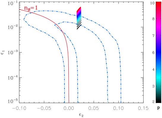
From these power spectra, assuming the conservation of the comoving curvature perturbation after Hubble exit (), the CMB anisotropies induced by the scalar and tensor perturbations can be derived and compared with the data. Using Markov-Chains-Monte-Carlo (MCMC) methods, one can extract constraints on the power spectra parameters, namely , and . Assuming a flat FLRW universe, the WMAP third year data lead to the posterior probability distributions plotted in Fig. 1.
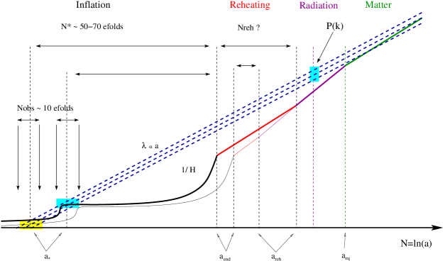
A great advantage of the slow-roll approach is that one does not need to specify an explicit model of inflation Martin:1999wa ; Liddle:1994dx ; Martin:1997zd ; Martin:2004um . The constraints verified by and apply to all (single field) inflationary models verifying the slow-rolling conditions and (see however Refs. Schwarz:2004tz ; deOliveira:2005mf ). However, using these results for a given model of inflation requires the knowledge of to determine the associated theoretical values of . As can be seen in Fig. 2, the value of depends on the number of efold during which the universe reheated before the radiation era. The reheating era depends on the microphysics associated with the decay of the inflaton field whose complexity renders the determination of difficult Felder:2000hj ; Kofman:1997yn ; Garcia-Bellido:1997wm ; Senoguz:2004vu ; Podolsky:2005bw ; Desroche:2005yt ; Allahverdi:2006wh . However, under reasonable assumptions, it has been shown in Ref. Liddle:2003as that typically , although these bounds may vary by a factor of two for extreme models. For the large field models represented in Fig. 1, the uncertainties on the reheating blur the theoretically predicted values of the slow-roll parameters (see the short segments in Fig. 1). Notice that the resulting errors in the remain small compared to the current CMB data accuracy, but this is not necessarily the case for other models, as for instance the small field models discussed in the following. The problem is expected to become even more significant with the next generation of more accurate CMB measurements.
Another difficulties that may show up with the slow-roll approach concern the existence of features in the inflaton potential. Although the current data support the almost scale invariance of the primordial power spectra, the presence of sharp localised deviations is still allowed by the data and might even be favoured Martin:2006rs ; Barriga:2000nk ; Martin:2003sg ; Martin:2004iv ; Martin:2004yi ; Easther:2004vq ; Hunt:2004vt ; Covi:2006ci . In the framework of field inflation, features in the power spectra generically result from transient non-slow-rolling evolution associated with sharp features in the inflation potential. In these cases, deriving analytical approximations for the perturbations require the use of more involved methods Martin:2002vn ; Casadio:2004ru ; Casadio:2005xv ; Casadio:2006wb . Let us also stress that one of the key ingredient rendering analytical methods attractive is the conservation of the comoving curvature perturbation on super-Hubble scales. As illustrated in Fig. 2, this allows one to identify the scalar and tensor power spectra deep in the radiation era, which seed the CMB anisotropies and structure formation, to the ones derived a few efolds after Hubble exit during inflation. However, as soon as inflation is driven by more than one field, the existence of isocurvature modes that may source after Hubble exit requires that the modes evolution should be traced till the end of reheating Gordon:2000hv . Although analytical methods can still be used, their use is restricted by their domain of validity Noh:2001ia ; DiMarco:2002eb ; DiMarco:2005nq .
The previous considerations suggest to use numerical methods to directly compute the inflationary perturbations and deduce the primordial power spectra. Numerical integrations in inflation are not new and have been used to test the validity of analytical approximations, or to derive the shape of the power spectra for some particular models Salopek:1988qh ; Grivell:1999wc ; Adams:2001vc ; Tsujikawa:2002qx ; Parkinson:2004yx ; Makarov:2005uh ; Chen:2006xj . However, with the advent of MCMC methods in cosmology, one may be interested in merging a full numerical integration of the perturbation during inflation with the CMB codes such as camb and cosmomc Lewis:1999bs ; Lewis:2002ah . The advantage of such an approach is that the inflationary parameters become part of the cosmological model under scrutiny. When compared with the data, one may expect to get consistent marginalised constraints on both the parameters entering the inflaton potential and the usual cosmological parameters describing the radiation and matter content of the observed universe. From a Bayesian point of view, this is the method that should be used when one is interested in assessing the probability of one model to explain the data (statistical evidence). Moreover, since the underlying approximation is just linear perturbation theory, one may consider without additional complications the treatment of non-standard models as those involving several fields. Let us mention that our objective is to use numerical methods in a well defined theoretical framework. For a given model, we use the CMB data to constrain the theoretical parameters and discuss the overall model ability to explain the data. Numerical (non-exact) methods have also been used in the context of the potential reconstruction problems where the goal is to constrain the shape of the inflaton potential along the observable window Peiris:2006sj ; Peiris:2006ug ; Kinney:2006qm (see Fig. 2).
However, as discussed before, to solve the cosmological perturbations from their creation as quantum fluctuations during inflation to now, it is necessary to model the reheating era. In fact, the importance of reheating for inflation is very similar to the importance of the reionisation for the CMB anisotropies. Although reionisation of the universe is a complex process, its basic effects on the CMB anisotropies can be modelled through the optical depth . Similarly, we will show that the basic effects induced by the reheating on the inflationary perturbations may be taken into account through a new parameter which has not been considered so far.
The plan is as follow. In a first section, the theoretical setup is introduced. We use the sigma-model formalism which allows an easy implementation of any scalar field inflation models in General Relativity and multi-scalar tensor theories. The equations of motion for the background fields and their perturbations are presented in the first section. Their numerical integration is the subject of the second part. After having introduced our modelisation of the reheating era, the last section illustrates the usefulness of the exact numerical method by an analysis of the third year WMAP data in the context of the small field models
2 Multifield inflation
It is out of the scope of this work to deal with all the inflationary models proposed so far. However, four-dimensional effective actions associated with many inflation models, and especially the ones being embedded in extra-dimensions, share the common feature that they involve several scalar fields that may be non-minimally coupled to gravity. This is for instance the case for the moduli associated with the position of the branes in various string-motivated inflation models Brax:2004xh . It is therefore convenient to consider an action that may generically drive the dynamics of both minimally and non-minimally coupled scalar fields, as in the sigma-model Damour:1992we ; Damour:1993id ; Koshelev:2005wk ; Ringeval:2005yn .
2.1 Sigma-model formalism
Denoting by the dimensionless scalar fields living on a sigma-model manifold with metric , we consider the action
| (4) |
where is the usual four dimensional metric tensor of determinant , the Ricci scalar and the field potential.
For instance, if and , this action describes a unique minimally coupled scalar field. In this case, the associated potential is and we recover the standard form
| (5) |
Another example is provided by the models of brane inflation where the inflaton field lives on the brane and a bulk field in the four-dimensional effective action couples to gravity in a non-minimal way Langlois:2002bb ; Maartens:2003tw ; Brax:2004xh . With , and , Eq. (4) can be recast into
| (6) | ||||
for
| (7) |
This action describes the dynamics, in the Einstein frame, of the field evolving in a potential in a scalar-tensor theory of gravity where is the scalar partner to the graviton Schimd:2004nq . The conformal function and the self-interaction potential depend on the brane setup considered Lukas:1998tt ; Lukas:1999yn ; Brax:2000xk ; Kobayashi:2002pw . In the general case, Eq. (4) can be used to describe multifield inflation in a multi-scalar tensor theory of gravity.
Differentiating the action (4) with respect to the metric leads to the Einstein equations
| (8) |
with the source terms
| (9) |
where
| (10) |
Similarly, the fields obey the Klein-Gordon-like equation
| (11) |
where denotes the Christoffel symbol on the field-manifold
| (12) |
and should be understood as the vector-like partial derivative of the potential
| (13) |
2.2 Background evolution
In a flat (FLRW) universe with metric
| (14) |
being the conformal time and and referring to the spatial coordinates, the equations of motion (8) and (11) simplify to
| (15) | ||||
| (16) | ||||
| (17) |
where a prime denotes differentiation with respect to the conformal time and is the conformal Hubble parameter. In terms of the efold time variable , the field equations can be decoupled from the metric evolution and one gets
| (18) | ||||
| (19) | ||||
| (20) |
a dot being a differentiation with respect to . We have introduced a velocity field
| (21) |
In fact, is the so-called adiabatic field introduced in Ref. Gordon:2000hv which describes the collective evolution of all the fields along the classical trajectory. From Eqs. (19) and Eq. (20) one may determine its equation of motion
| (22) |
with and where the are unit vectors along the field trajectory:
| (23) |
In the Einstein frame, inflation occurs for , or in terms of the first Hubble flow function, for111Notice that this does not imply that the universe is accelerating in the string frame and one has to verify that there are enough efolds of inflation to solve the homogeneity and flatness issues in that frame Ringeval:2005yn ; Esposito-Farese:2000ij ; Martin:2005bp .
| (24) |
The multifield system induces an accelerated expansion of the universe if the resulting adiabatic field velocity remains less than . According to Eq. (20), the term in acts as a relativistic-like inertia for the fields evolution and thus (for a positive potential). In this equation, the first term on the left hand side may be interpreted as a covariant acceleration on the curved field manifold, the second as a constant friction force and the right hand side as a driving force deriving from the potential . In fact, we recover the well-known attractor behaviour of the inflationary evolution: whatever the initial fields velocity, the friction term ensures that the terminal velocity of the fields will be, after a transient regime,
| (25) |
Analytical integration of the previous expression is at the basis of the slow-roll approximation when the effective potential is flat enough. In the general case, the driving force is always pushing the fields towards the minimum of . Let us note that this is why the monomial potentials are actually “flat” for the large field values: which goes to zero for .
2.3 Linear perturbations
Scalar modes
In the longitudinal gauge, the scalar perturbations (with respect to the rotations of the three-dimensional space) of the FLRW metric can be expressed as
| (26) |
where and are the Bardeen potentials. With the field perturbations, the Einstein equations perturbed at first order read
| (27) | ||||
| (28) | ||||
| (29) |
where use has been made of from the perturbed Einstein equation with . For flat spacelike hypersurfaces,
| (30) |
Similarly, the perturbed Klein-Gordon equations read
| (31) |
As discussed in the introduction, if there is more than one scalar field involved, the entropy perturbation modes can source the adiabatic mode even after Hubble exit. The equation governing the evolution of the comoving curvature perturbation can be obtained from Eqs. (2.3) to (2.3), using the background equations. Firstly, the Bardeen potential verifies
| (32) |
Using the geometrical definition for the comoving curvature perturbation Martin:1997zd
| (33) |
Eq. (28) yields
| (34) |
where the adiabatic perturbation is also the resulting perturbation of all fields projected onto the classical trajectory [see Eqs. (21) and (23)]:
| (35) |
The dynamical equation (32) now exhibits couplings between the adiabatic and entropy modes
| (36) |
which can be recast into
| (37) |
The orthogonal projector is defined by
| (38) |
where is the first fundamental form of the one-dimensional manifold defined by the classical trajectory Carter:1997pb . Clearly, the comoving curvature perturbation on super-Hubble scales for which is only sourced by the entropy perturbations defined as the projections of all field perturbations on the field-manifold subspace orthogonal to the classical trajectory. If, on the contrary, there is a single field involved during inflation, then these terms vanish and we recover that remains constant after Hubble exit.
Tensor modes
In the Einstein frame, the scalar and tensor degrees of freedom are decoupled. Therefore, the equation of evolution for the tensor modes remains the same as in General Relativity. For a flat perturbed FLRW metric
| (39) |
where is a traceless and divergenceless tensor
| (40) |
one gets Mukhanov:1990me ; Liddle:1993fq
| (41) |
Primordial power spectra
The initial conditions for the cosmological perturbations require the knowledge of the two-point correlation functions for all of the observable scalar and tensor modes deep in the radiation era. In Fourier space, these are just the power spectra associated with the values taken by the adiabatic and entropy perturbations at the end of the reheating, i.e.
| (42) |
where stands for or the entropy modes. Similarly, taking into account the polarisation degrees of freedom, the tensor power spectrum reads
| (43) |
3 Numerical method
3.1 Integrating the background
As suggested by the form of Eqs. (18) to (20), it is convenient to use the number of efold as the integration variable. In fact, the background evolution only requires the integration of the fields equation of motion (20). From the Cauchy theorem, the solution is unique provided all the and are given at . Plugging the solutions for into Eq. (18) uniquely determine the Hubble parameter and thus the geometry during inflation.
Initial conditions
However, as previously mentioned, the attractor behaviour induced by the friction term erases any effect associated with the initial field velocities after a few efolds. This is the very reason why initial conditions in inflation are essentially related to the initial field values only. On the numerical side, the attractor ensures the stability of almost all forward numerical integration schemes222as well as the instability of backward integrations.. In the following, we have used a Runge-Kutta integration method of order five and the initial field velocities have been chosen on the attractor by setting
| (44) |
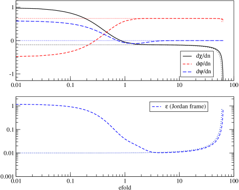
The robustness of the attractor during inflation may be quantified by comparing the numerical solutions obtained from various arbitrary choices of the initial field velocities, at fixed value of . As an illustration, we have plotted in Fig. 3 the efold evolution of in a brane inflation model involving three scalar fields, two of them are non-minimally coupled to gravity and represent the position of two branes in a five-dimensional bulk (see Ref. Ringeval:2005yn ). As can be seen on this plot, all the fields are on the attractor after a few efolds.
End of inflation
From the above initial conditions the fields evolve toward the minimum of the potential while the expansion of the universe accelerates as long as . It would therefore be natural to define the end of inflation by the efold at which . However, this is usually not the end of the fields evolution since they have not yet reached the minimum of the potential. On the contrary, just signals that the kinetic terms in Eq. (4) start to dominate over the potential. Since the expansion factor is decelerating for , this late stage evolution takes place during a few efolds and the fields rapidly reach the minimum of the potential. In the standard picture, the fields oscillate around the minimum of the potential and decay through parametric resonances into the relativistic fluids present during the radiation era Kofman:1997yn ; Turner:1983he (see Fig. 4)

The details of the reheating process are very model dependent and require the knowledge of all the couplings between the inflaton and the standard model particles Bassett:2005xm . This implies that the number of efolds the universe reheated also depends on the model at hand. Another complications come in multifield inflationary models in which the end of inflation and the reheating may be triggered by tachyonic instabilities. In these cases the condition is not longer relevant and one should rather introduce a limiting field value to classically define the beginning of the reheating era (and the end of inflation).
Following the previous discussion, our phenomenological approach to the end of inflation is to assume an instantaneous transition to the reheating era. The efold at which the transition occurs is either determined by the condition or when the relevant field cross a limiting value ; the choice being made according to the inflation model we are interested in. The value of may be given by the underlying microphysics or considered as an additional parameter of the inflation model. For instance, as can be seen in Fig. 4, it is convenient to define the end of inflation for the large field models by : the field evolution afterwards, oscillations around the minimum of the potential and subsequent decay, is supposed to be part of the reheating stage.
Knowing the fields value from to , the background geometry is given by Eqs. (18) and (19) and we can now numerically integrate the linear perturbations on the same efold range. As discussed in the introduction, the link with the cosmological perturbations observed today still requires a reheating model that will be introduced in Sect. 4.1.
3.2 Integrating the perturbations
As for the background, we have chosen to integrate the linear perturbations in efold time. Focusing on the scalar perturbations, their dynamics is driven by the Einstein and Klein-Gordon equations given in Sect. 2.3. These ones are however redundant due to the stress energy conservation already included in the Bianchi identities. As a result, it is necessary to integrate only a subset of Eqs. (2.3) to (2.3). Although the Bardeen potential could be explicitly expressed in terms of the field perturbations only, such an expression is singular in the limit and , which is not appropriate for a numerical integration (see below). It is more convenient to simultaneously integrate the second order equations (2.3) and (32). Recast in efold time, they read
| (45) | ||||
| (46) |
The constraint equations (2.3) and (28) being first integrals of the above equations, there is still an integration constant that should be set to restore the equivalence to the full set of Einstein and Klein-Gordon equations. This one can be fixed by choosing the appropriate initial conditions at for the Bardeen potential . Setting all the and , the initial conditions for the Bardeen potential are indeed uniquely given by Eq. (2.3) and (28). In efold time, one gets
| (47) | ||||
these expressions being evaluated at the initial efold time. As a result, the linear perturbations of both the fields and metric are uniquely determined by the initial conditions and . As discussed in the next section, the initial conditions are set on sub-Hubble scales for which ensuring the regularity of Eqs. (47).
Quantum initial conditions
In the context of single field inflation, the initial conditions for the linear perturbations are given by the quantum fluctuations of the field-metric system on sub-Hubble scales . In this limit, the perturbations decouple from the expansion of the universe and a field quantisation can be performed along the lines described in Refs. Mukhanov:1990me ; Martin:2004um . The canonically normalised quantum degrees of freedom are encoded in the Mukhanov-Sasaki variable
| (48) |
with for single field models. In terms of , the equation of motion (2.3) can be recast into
| (49) |
showing that in the small scales limit , the quantity follows the dynamics of a free scalar field. Assuming a Bunch-Davies vacuum, has a positive energy plane wave behaviour on small scales and in Fourier space one gets
| (50) |
This solution uniquely determines the subsequent evolution of the perturbations during inflation and will be our starting point for the numerical integration. According to Eq. (47), provided the initial conditions are set in the limit , Eq. (50) is also the small scales behaviour of the rescaled adiabatic field perturbations .
For a multifield system the previous results can be generalised and the quantum modes identify with the adiabatic perturbations together with the canonically normalised entropy modes introduced in Sect. 2.3. In fact, if the original fields are already canonically normalised, i.e. , and independent dynamical variables in the small scales limit, the adiabatic and entropy perturbations can be obtained from the original field perturbations by local rotations on the -dimensional field manifold Gordon:2000hv ; DiMarco:2002eb ; Ringeval:2005yn . In this case, denoting by the adiabatic and entropy perturbations, with the convention , one has
| (51) |
where is an instantaneous rotation matrix, , depending on the background quantities only. Under these assumptions, the quantum modes are independent in the small scales limit and their two point correlators reduce to
| (52) |
being the free field power spectrum given by the square modulus of Eq. (50). Consequently, all the correlators between the original field perturbations inherit these initial conditions:
| (53) |
The previous results can be generalised for the sigma-models with a diagonal metric non equal to the identity by the transformation (no summation). In the general case, the transformation matrix would mix all the fields and the cross correlators. However, since it is always possible to diagonalise through a field redefinition, we will now assume without lost of generality that is diagonal.
Defining the normalised quantum modes by
| (54) |
with evaluated along the background solution, in the small scales limit Eq. (50) can be recast into the initial conditions
| (55) |
up to a phase factor. In terms of the field perturbations, the initial conditions in efold time therefore read
| (56) | ||||
The efold at which these initial conditions should be set has not been specified yet. In fact, the limit would correspond to the infinite past and does not make sense for non-eternal field inflation models333Eternal inflation may occur when the quantum fluctuations on Hubble length scales become dominant over the classical field evolution and the semi-classical approach used here would no longer be valid, at least in the self-reproducing regime.. However, by definition of , the condition is already satisfied a few efolds before Hubble exit. For all inflation models lasting more than efolds, it would be natural to set the initial conditions for the perturbations at the beginning of inflation (see Fig. 2).
Choosing is however not appropriate for a numerical integration. Indeed, according to the initial values of the background fields, the total number of efolds can be much greater than . In such cases, most of the computing time for the perturbations would be spent into the deep sub-Hubble regime for which the modes behave as free plane waves. It is rather more convenient to set the initial conditions “closer” to the time at which a given mode cross the Hubble radius . Following Ref. Salopek:1988qh , a simple choice is to define for each mode according to
| (57) |
being a constant verifying and characterising the decoupling limit. Strictly speaking, this choice introduces small trans-Planckian-like interferences between the modes444In the free field limit, a more accurate choice for is . This definition maintains the phase factor in Eq. (50) independent of on the initial hypersurface. which remain however negligible provided is big enough Niemeyer:2002kh .
Mode integration
For each perturbation mode of wavenumber , Eqs. (3.2) and (46) are numerically solved by setting the initial conditions (56) at the efold , solution of Eq. (57). In order to significantly speed-up the numerical integration, instead of using the already computed background solution it is more convenient to integrate both the background and the perturbations simultaneously555For direct numerical integrations, each step requires various forward and backward evaluations of the background functions. If these ones are not analytically known but precomputed, one has to use spline and interpolation methods which are heavily time-consuming.. This can be done along the following steps.
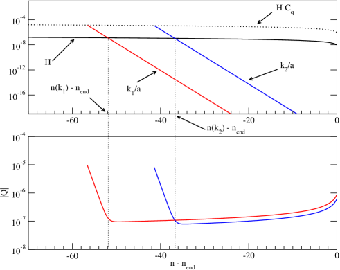
Firstly, Eq. (57) is solved to determine for the largest wavelength mode we are interested in. The background equations (20) and are then integrated from to . At that efold, Eqs. (20), (3.2) and (46) are simultaneously integrated till the end of inflation at . This process is iterated for each of the mode wanted. However, to speed-up the integration, it is enough to re-integrate the background from to rather than from before switching on the perturbations (see Fig. 5). Such an integration gives the value of all the field and metric perturbations at the end of inflation . In principle, the power spectra can then be deduced by using Eq. (42).
Primordial power spectra
For a multifield system, since the perturbation modes are supposed to be independent deep under the Hubble radius, they can be considered, from a classical point of view, as independent stochastic variables. As a result, the power spectra at the end of inflation are no longer given by Eq. (42) but should be computed as Tsujikawa:2002qx
| (58) |
where, as before, stands for the observable perturbations one is interested in. The can be the field perturbations themselves but it is more customary for CMB analysis to use the comoving curvature perturbation and the rescaled entropic perturbations (). The index “” in Eq. (58) refers to the independent initial conditions obtained by setting only one perturbation mode in the Bunch-Davies vacuum at , the other vanishing. Notice that we have not explicitly written the entropy modes since various definitions are used in the literature. The definition of the entropy modes through the standard orthogonalisation procedure along the field trajectory can be found in Refs. Gordon:2000hv ; DiMarco:2002eb and has the advantage to give canonically normalised perturbations. Another definitions introduce a reference field and define the entropy perturbations to be the relative perturbations of the other fields with respect to it. These differences come from the fact that one has to specify how the fields decay after inflation to know between which cosmological fluids entropy perturbations may exist. For instance, if all the cosmological fluids observed today are produced by the decay of one field only, then, although entropy perturbations exist during inflation, they are usually not observable afterwards Weinberg:2004kf ; Lemoine:2006sc . Their only effect would be to break the conservation of on super-Hubble scale thereby requiring the integration of all the perturbations till the end of inflation to determine the power spectrum.
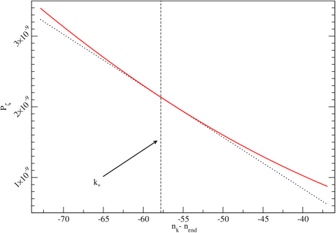
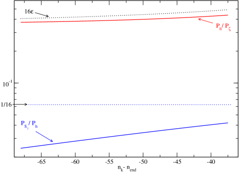
As an illustration, Fig. 6 shows the exact numerical power spectrum for the comoving curvature perturbation for the single field chaotic model . As can be seen on this plot, although the exact power spectrum differs from its first slow-roll approximated version given by Eq. (2), the differences remain small on a efold observable range. Another example involving entropy perturbations is plotted in Fig. 7 for a two fields model of inflation. The presence of one entropy mode breaks the conservation of on super-Hubble scale and the so-called consistency check of inflation [see Eqs. (2) and (3) at zero order].
Tensor perturbations
Since in the Einstein frame the tensor and scalar degrees of freedom are decoupled, the numerical integration of the tensor modes does not present any difficulties. The equation of motion (41) can be recast into the equation of a parametric oscillator by defining the canonical mode function satisfying the deep sub-Hubble initial conditions (50) for a Bunch-Davies vacuum Mukhanov:1990me . The power spectrum is readily obtained by evaluating Eq. (43) at the end of inflation.
Physical wavenumbers
Up to now, one may have noticed that all the power spectra have been plotted with respect to and not with respect to the values of . For astrophysical purpose, one needs to know the correspondence between the comoving appearing in the above equations and the physical wavenumbers measured today , whose typical unit is the . As it appears in the initial conditions (56), rendering explicit requires the knowledge of , i.e. the redshift associated with the end of inflation. As discussed in Sect. 1, this can only being done if one knows the number of efolds during which the universe reheated. Let us also notice that the physics involved in the quantum generation of cosmological perturbations appears through these very numbers: are the wavenumbers measured today, usually of size, expressed in unit of the Planck mass with [see Eq. (56)].
4 Application to CMB data analysis
Fig. 2 makes clear that from the integration of the perturbations described in the previous section, their power spectra are known at the end of inflation. These primordial correlations then evolve through the reheating, radiation and matter era to shape the universe into its current state. The theory of cosmological perturbations precisely predicts how such linear perturbations evolve in a FLRW universe from the tightly coupled regime deep inside the radiation era to today. As a result, we still have to know how the power spectra are modified through the reheating era. As already mentioned, reheating is very model dependant and a detailed analysis is out of the scope of our current approach. Instead, remembering that the objective is to use the CMB anisotropies measurements as a probe to get information on the primordial correlations, we introduce a basic model of reheating described by some phenomenological parameters.
4.1 Reheating
Assuming that perturbations on super-Hubble scales are not significantly modified till the beginning of the radiation era666Although such an assumption is motivated by the fact that the physical processes involved during reheating are sub-Hubble, this assumption may not longer be true in presence of entropy modes., the reheating may influence the observed power spectra through its effects on (see Fig. 2). For instantaneous transitions between inflation, the reheating era and the radiation era Liddle:2003as , one has
| (59) |
where , and are respectively the scale factor at the end of inflation, at the end of reheating and at equality between the energy density of radiation and the energy density of matter. The redshift of equality can be expressed in terms of the density parameter of radiation today and the Hubble parameter today . Moreover, during the radiation era , and Eq. (59) can be recast into
| (60) |
where denotes the total energy density at the end of the reheating era. It is clear that the first two terms depend on the physics involved during the reheating. For instance, they would only depend on the energy density at the end of inflation for a radiation-like reheating era. This suggests to introduce a phenomenological parameter Martin:2006rs
| (61) |
From this parameter, the quantity entering the equations of motion for the perturbations (3.2) and (46) can be evaluated in terms of the values measured today
| (62) |
and similarly for the initial conditions in Eq. (56).
4.2 CMB anisotropies
For a given value of , the primordial power spectra deep in the radiation era are now uniquely determined by the numerical integration described in Sect. 3 and can be used as initial conditions for the subsequent evolution of the perturbations.
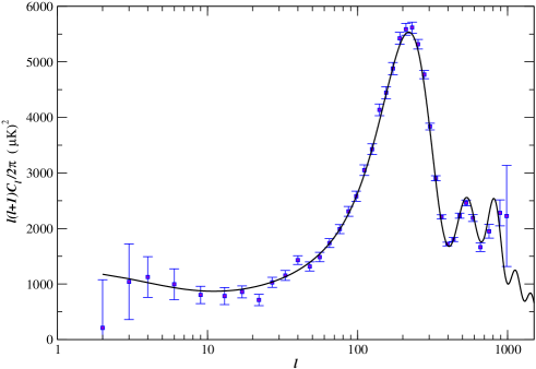
The integration of the cosmological perturbations through the radiation and matter era, as well as the resulting CMB anisotropies, have been performed by using a modified version of the camb code Lewis:1999bs . The model parameters involved are both the inflation parameters and the usual cosmological parameters describing the FLRW model at late time. For instance, for a CDM universe experiencing large field inflation in its earliest times, there are two parameters fixing the potential , one parameter describing the reheating era , plus the four cosmological base parameters: the number density of baryons , of cold dark matter , the Hubble parameter today and the redshift of reionisation of the universe Lewis:2002ah . Let us recap that we have defined the end of large field inflation by . Combined with the existence of the attractor during inflation, this ensures that is fixed by the potential parameters [see Eq. (25)]. The resulting angular power spectrum for the CMB temperature fluctuations is represented in Fig. 8 for a fiducial set of the parameters.
The next step is to use CMB measurements to constrain the models. For this purpose, the parameter space can be sampled by using Markov Chain Monte Carlo (MCMC) methods as implemented in the cosmomc code Lewis:2002ah to extract the probability distributions satisfied by the model parameters. In the next section, we illustrate such a procedure for the CDM model born under small field inflation by using the WMAP third year data Page:2006hz ; Hinshaw:2006ia ; Jarosik:2006ib .
4.3 WMAP3 constraints on small field models
Small field inflation can be described by the action (5) when the potential reads
| (63) |
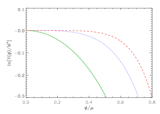
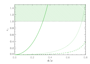
The inflation model parameters are the energy scale , the power and the vacuum expectation value scale . As can be seen in Fig. 9, inflation proceeds for small initial field values and stops when . Notice that the potential in Eq. (63) is negative for which means that the above description is no longer correct. This is however not an issue since it occurs well after the end of inflation and the basic effects of the reheating are already encoded in our extra parameter .
Observable parameters
Since flatness is inherited from inflation, the CDM cosmological model is described by the density parameters associated with the different cosmological fluids: , plus the Hubble parameter today . The cosmological constant is fixed by . However, in order to minimise the parameter degeneracies with respect to the CMB angular power spectra, it is more convenient to perform the MCMC sampling on the equivalent set of parameters , , the optical depth and the quantity which measures the ratio of the sound horizon to the angular diameter distance ( is the reduced Hubble parameter today) Lewis:2002ah .
Similarly for the potential parameters, as can be seen in Eqs. (2) and (3), the overall amplitude of the CMB anisotropies is proportional to the Hubble parameter squared and thus to the potential [see Eq. (18)]. Since the amplitude of the cosmological perturbations is a well measured quantity, the data may be more efficiently used by directly sampling the primordial amplitude of the scalar power spectrum instead of ( being a fixed observable wavenumber: ).
However, the numerical method used to integrate the perturbations during inflation requires the input of a numerical value for to predict the value of . In fact, one can use the trick described in Ref. Martin:2006rs : under a rescaling , the power spectrum scales as at fixed . The idea is therefore to integrate the perturbations with an artificial normalisation of the potential, for instance , and then analytically rescale from unity to its physical value that would be associated with . The required value of is given by the ratio , where is the amplitude of the scalar power spectrum stemming from the numerical integration with and evaluated at . Still, it is not really straightforward to determine since both and change simultaneously. The last subtlety is to remark that if instead of considering fixed, one considers the rescaling of at fixed , with defined by
| (64) |
The parameters and differ only by , the energy density at the end of inflation which is uniquely determined from , and . It will be therefore more convenient to sample the model parameters and (together with and ) rather than and .
Priors
The prior probability distributions for the base cosmological parameters , , and have been chosen as wide top hat uniform distribution centred over their current preferred value Spergel:2006hy ; Lewis:2002ah .
Concerning the inflaton potential parameters, their priors can be chosen according to various theoretical prejudices Martin:2006rs . Since is related to the energy scale during inflation, a uniform prior has been considered around a value compatible with the amplitude of the cosmological perturbations: . For the scale associated with the vacuum expectation value of , we have considered two priors. The first includes smaller and larger values than the Planck mass: . The second prior is also uniform but include values much larger than the Planck mass: . Finally, a uniform prior is chosen for the power on ( is a particular case, see Ref. Martin:2006rs ).
It remains to express our prior knowledge on the reheating parameter . As previously mentioned, we are assuming that gravity can still be described classically which only makes sense if the energy densities involved remain smaller than the Planck energy scale, namely for . On the other side of the energy spectrum, the success of big-bang nucleosynthesis (BBN) requires that the universe is radiation dominated at that time, thus with (and ). Moreover, we will assume that during reheating the expansion of the universe can be described as dominated by a cosmological fluid of pressure and energy density . In this case, in order to satisfy the strong and dominant energy conditions in General Relativity, one has (notice that would be inflation). From Eqs. (61) and (64), the resulting bounds read
| (65) |
and an uniform prior on have been chosen in between.
Results
The data sets used to constrain the small field CDM model are the WMAP third year data together with the Hubble Space Telescope (HST) measurements ( Freedman:2000cf ) and a top hat prior on the age of the universe between and .
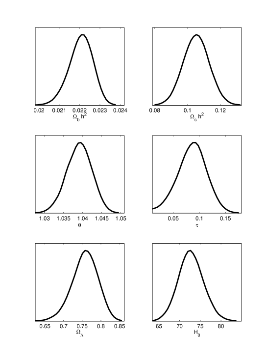
The resulting marginalised posterior probability distributions for the base cosmological parameters are represented in Fig. 10. They are not significantly affected by the various prior choices on and their corresponding mean values and confidence intervals are compatible with the current state or art Spergel:2006hy .
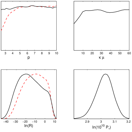
The constraints obtained on the small field inflation parameters are showed in Fig. 11. As expected, the allowed range for the power spectra amplitude is narrow. Concerning the above panels their interpretation require some precautions. Indeed, the probability that takes small values depends on our theoretical prejudice on how big the field expectation value of the inflaton may be. If is allowed to be much greater than then all are equiprobable. On the other hand, if cannot take values bigger than then small field inflation models with are disfavoured. The posterior shows on its own that, independently of the values, is slightly preferred by the data. Since these posteriors are marginalised over the other parameters, the previous statements are necessarily robust with respect to any reheating model, in the framework of our modelisation.
But more than being a nuisance parameter, Fig. 11 shows that is also mildly constrained by the data: the probability distribution of has a lower bound slightly above the prior given by Eq. (65). Although this is not obvious, the upper cut-off seen in the posterior comes from the upper bound of Eq. (65) (see Ref. Martin:2006rs for a more detailed discussion). For in , we finally obtain at confidence level777The dependence of the posterior distribution with respect to the prior disappears as soon as is allowed to be greater than .
| (66) |
Plugging this inequality into Eq. (64) constrains some properties of the reheating era. This result can be understood by looking at Fig. 2. Since varying the reheating properties allow the observable window to move along the inflaton potential, it is not surprising that some part of the potential may be preferred from a data point of view. For the small field models, a more involved analysis would show that the spectral index of the scalar power spectrum gets away from what is allowed by the data when becomes too small Martin:2006rs . This is precisely why the current WMAP data lead to the bound (66).
5 Conclusion
As a conclusion, we would like to discuss the future directions associated with the possibility of constraining some basic properties of the reheating era with the CMB data.
In the small field CDM inflation analysed in the previous section, the bound found in Eq. (66) can be further explored by being more specific on the way the universe reheated. As a toy example, if one assumes that reheating proceeded with a constant equation of state , then Eq. (64) simplifies into
| (67) |
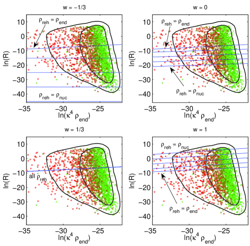
In the parameter plane , for a given value of the reheating energy, Eq. (67) corresponds to a straight line. In Fig. 12, five of these lines exploring the range have been superimposed to the two-dimensional probability distributions associated with the small field model, and this for four different equations of state having and , respectively.
At can be seen on the top left frame, for , low values of the reheating temperature are out of the confidence contours. From a more robust analysis using importance sampling, one would find in that case that, at of confidence, Martin:2006rs . Of course this bound is not really impressive and close to the limits already set by BBN, moreover, it holds only for small field models and a quite extreme equation of state. However, is shows that it is already possible to get some information on the reheating era in a given model of inflation from the CMB data only. This is precisely on this point that particle physics models may be decisive. Indeed, once the inflaton couplings to the other particles are specified, the properties of the reheating era are fixed and a given particle physics model would appear as one curve parametrised by some coupling constants in the plane of Fig. 12. With the incoming flow of more accurate cosmological data, this may be an interesting way of constraining inflation as well as particle physics at very high energy.
Acknowledgments
I would like to thank Jérôme Martin for his comments on the manuscript as well as the organisers of the “Inflation+25” conference for the outstanding scientific atmosphere that took place during this colloquium. This work was partially supported by the Belgian Federal Office for Scientific, Technical and Cultural Affairs through the Inter-University Attraction Pole grant P6/11.
References
- (1) D. N. Spergel et. al., Wilkinson microwave anisotropy probe (wmap) three year results: Implications for cosmology, astro-ph/0603449.
- (2) B. A. Bassett, S. Tsujikawa, and D. Wands, Inflation dynamics and reheating, Rev. Mod. Phys. 78 (2006) 537–589, [astro-ph/0507632].
- (3) R. Allahverdi, K. Enqvist, J. Garcia-Bellido, and A. Mazumdar, Gauge invariant mssm inflaton, Phys. Rev. Lett. 97 (2006) 191304, [hep-ph/0605035].
- (4) R. Allahverdi, K. Enqvist, J. Garcia-Bellido, A. Jokinen, and A. Mazumdar, Mssm flat direction inflation: Slow roll, stability, fine tunning and reheating, hep-ph/0610134.
- (5) S. H. H. Tye, Brane inflation: String theory viewed from the cosmos, hep-th/0610221.
- (6) D. J. Schwarz, C. A. Terrero-Escalante, and A. A. Garcia, Higher order corrections to primordial spectra from cosmological inflation, Phys. Lett. B517 (2001) 243–249, [astro-ph/0106020].
- (7) D. H. Lyth and A. Riotto, Particle physics models of inflation and the cosmological density perturbation, Phys. Rept. 314 (1999) 1–146, [hep-ph/9807278].
- (8) V. F. Mukhanov, H. A. Feldman, and R. H. Brandenberger, Theory of cosmological perturbations. part 1. classical perturbations. part 2. quantum theory of perturbations. part 3. extensions, Phys. Rept. 215 (1992) 203–333.
- (9) E. D. Stewart and D. H. Lyth, A more accurate analytic calculation of the spectrum of cosmological perturbations produced during inflation, Phys. Lett. B302 (1993) 171–175, [gr-qc/9302019].
- (10) J. Martin and D. J. Schwarz, The precision of slow-roll predictions for the cmbr anisotropies, Phys. Rev. D62 (2000) 103520, [astro-ph/9911225].
- (11) J. Martin and C. Ringeval, Inflation after wmap3: Confronting the slow-roll and exact power spectra with cmb data, JCAP 0608 (2006) 009, [astro-ph/0605367].
- (12) A. R. Liddle, P. Parsons, and J. D. Barrow, Formalizing the slow roll approximation in inflation, Phys. Rev. D50 (1994) 7222–7232, [astro-ph/9408015].
- (13) J. Martin and D. J. Schwarz, The influence of cosmological transitions on the evolution of density perturbations, Phys. Rev. D57 (1998) 3302–3316, [gr-qc/9704049].
- (14) J. Martin, Inflationary cosmological perturbations of quantum- mechanical origin, Lect. Notes Phys. 669 (2005) 199–244, [hep-th/0406011].
- (15) D. J. Schwarz and C. A. Terrero-Escalante, Primordial fluctuations and cosmological inflation after wmap 1.0, JCAP 0408 (2004) 003, [hep-ph/0403129].
- (16) H. P. de Oliveira and C. A. Terrero-Escalante, Troubles for observing the inflaton potential, JCAP 0601 (2006) 024, [astro-ph/0511660].
- (17) G. N. Felder et. al., Dynamics of symmetry breaking and tachyonic preheating, Phys. Rev. Lett. 87 (2001) 011601, [hep-ph/0012142].
- (18) L. Kofman, A. D. Linde, and A. A. Starobinsky, Towards the theory of reheating after inflation, Phys. Rev. D56 (1997) 3258–3295, [hep-ph/9704452].
- (19) J. Garcia-Bellido and A. D. Linde, Preheating in hybrid inflation, Phys. Rev. D57 (1998) 6075–6088, [hep-ph/9711360].
- (20) V. N. Senoguz and Q. Shafi, Reheat temperature in supersymmetric hybrid inflation models, Phys. Rev. D71 (2005) 043514, [hep-ph/0412102].
- (21) D. I. Podolsky, G. N. Felder, L. Kofman, and M. Peloso, Equation of state and beginning of thermalization after preheating, Phys. Rev. D73 (2006) 023501, [hep-ph/0507096].
- (22) M. Desroche, G. N. Felder, J. M. Kratochvil, and A. Linde, Preheating in new inflation, Phys. Rev. D71 (2005) 103516, [hep-th/0501080].
- (23) R. Allahverdi and A. Mazumdar, Towards a successful reheating within supersymmetry, hep-ph/0603244.
- (24) A. R. Liddle and S. M. Leach, How long before the end of inflation were observable perturbations produced?, Phys. Rev. D68 (2003) 103503, [astro-ph/0305263].
- (25) J. Barriga, E. Gaztanaga, M. G. Santos, and S. Sarkar, On the apm power spectrum and the cmb anisotropy: Evidence for a phase transition during inflation?, Mon. Not. Roy. Astron. Soc. 324 (2001) 977, [astro-ph/0011398].
- (26) J. Martin and C. Ringeval, Superimposed oscillations in the wmap data?, Phys. Rev. D69 (2004) 083515, [astro-ph/0310382].
- (27) J. Martin and C. Ringeval, Addendum to “superimposed oscillations in the wmap data?”, Phys. Rev. D69 (2004) 127303, [astro-ph/0402609].
- (28) J. Martin and C. Ringeval, Exploring the superimposed oscillations parameter space, JCAP 0501 (2005) 007, [hep-ph/0405249].
- (29) R. Easther, W. H. Kinney, and H. Peiris, Observing trans-planckian signatures in the cosmic microwave background, JCAP 0505 (2005) 009, [astro-ph/0412613].
- (30) P. Hunt and S. Sarkar, Multiple inflation and the wmap ’glitches’, Phys. Rev. D70 (2004) 103518, [astro-ph/0408138].
- (31) L. Covi, J. Hamann, A. Melchiorri, A. Slosar, and I. Sorbera, Inflation and wmap three year data: Features have a future!, Phys. Rev. D74 (2006) 083509, [astro-ph/0606452].
- (32) J. Martin and D. J. Schwarz, Wkb approximation for inflationary cosmological perturbations, Phys. Rev. D67 (2003) 083512, [astro-ph/0210090].
- (33) R. Casadio, F. Finelli, M. Luzzi, and G. Venturi, Improved wkb analysis of cosmological perturbations, Phys. Rev. D71 (2005) 043517, [gr-qc/0410092].
- (34) R. Casadio, F. Finelli, M. Luzzi, and G. Venturi, Higher order slow-roll predictions for inflation, Phys. Lett. B625 (2005) 1–6, [gr-qc/0506043].
- (35) R. Casadio, F. Finelli, A. Kamenshchik, M. Luzzi, and G. Venturi, Method of comparison equations for cosmological perturbations, JCAP 0604 (2006) 011, [gr-qc/0603026].
- (36) C. Gordon, D. Wands, B. A. Bassett, and R. Maartens, Adiabatic and entropy perturbations from inflation, Phys. Rev. D63 (2001) 023506, [astro-ph/0009131].
- (37) H. Noh and J.-c. Hwang, Inflationary spectra in generalized gravity: Unified forms, Phys. Lett. B515 (2001) 231–237, [astro-ph/0107069].
- (38) F. Di Marco, F. Finelli, and R. Brandenberger, Adiabatic and isocurvature perturbations for multifield generalized einstein models, Phys. Rev. D67 (2003) 063512, [astro-ph/0211276].
- (39) F. Di Marco and F. Finelli, Slow-roll inflation for generalized two-field lagrangians, Phys. Rev. D71 (2005) 123502, [astro-ph/0505198].
- (40) D. S. Salopek, J. R. Bond, and J. M. Bardeen, Designing density fluctuation spectra in inflation, Phys. Rev. D40 (1989) 1753.
- (41) I. J. Grivell and A. R. Liddle, Inflaton potential reconstruction without slow-roll, Phys. Rev. D61 (2000) 081301, [astro-ph/9906327].
- (42) J. A. Adams, B. Cresswell, and R. Easther, Inflationary perturbations from a potential with a step, Phys. Rev. D64 (2001) 123514, [astro-ph/0102236].
- (43) S. Tsujikawa, D. Parkinson, and B. A. Bassett, Correlation-consistency cartography of the double inflation landscape, Phys. Rev. D67 (2003) 083516, [astro-ph/0210322].
- (44) D. Parkinson, S. Tsujikawa, B. A. Bassett, and L. Amendola, Testing for double inflation with wmap, Phys. Rev. D71 (2005) 063524, [astro-ph/0409071].
- (45) A. Makarov, On the accuracy of slow-roll inflation given current observational constraints, Phys. Rev. D72 (2005) 083517, [astro-ph/0506326].
- (46) X. Chen, R. Easther, and E. A. Lim, Large non-gaussianities in single field inflation, astro-ph/0611645.
- (47) A. Lewis, A. Challinor, and A. Lasenby, Efficient computation of cmb anisotropies in closed frw models, Astrophys. J. 538 (2000) 473–476, [astro-ph/9911177].
- (48) A. Lewis and S. Bridle, Cosmological parameters from cmb and other data: a monte- carlo approach, Phys. Rev. D66 (2002) 103511, [astro-ph/0205436].
- (49) H. Peiris and R. Easther, Slow roll reconstruction: Constraints on inflation from the 3 year wmap dataset, JCAP 0610 (2006) 017, [astro-ph/0609003].
- (50) H. Peiris and R. Easther, Recovering the inflationary potential and primordial power spectrum with a slow roll prior, astro-ph/0603587.
- (51) W. H. Kinney, E. W. Kolb, A. Melchiorri, and A. Riotto, Inflation model constraints from the wilkinson microwave anisotropy probe three-year data, Phys. Rev. D74 (2006) 023502, [astro-ph/0605338].
- (52) P. Brax, C. van de Bruck, and A.-C. Davis, Brane world cosmology, Rept. Prog. Phys. 67 (2004) 2183–2232, [hep-th/0404011].
- (53) T. Damour and G. Esposito-Farese, Tensor multiscalar theories of gravitation, Class. Quant. Grav. 9 (1992) 2093–2176.
- (54) T. Damour and K. Nordtvedt, Tensor - scalar cosmological models and their relaxation toward general relativity, Phys. Rev. D48 (1993) 3436–3450.
- (55) N. A. Koshelev, Adiabatic and entropy perturbations in inflationary models based on non-linear sigma model, Grav. Cosmol. 10 (2004) 289–294, [astro-ph/0501600].
- (56) C. Ringeval, P. Brax, v. de Bruck, Carsten, and A.-C. Davis, Boundary inflation and the wmap data, Phys. Rev. D73 (2006) 064035, [astro-ph/0509727].
- (57) D. Langlois, Brane cosmology: An introduction, Prog. Theor. Phys. Suppl. 148 (2003) 181–212, [hep-th/0209261].
- (58) R. Maartens, Brane-world gravity, Living Rev. Rel. 7 (2004) 7, [gr-qc/0312059].
- (59) C. Schimd, J.-P. Uzan, and A. Riazuelo, Weak lensing in scalar-tensor theories of gravity, Phys. Rev. D71 (2005) 083512, [astro-ph/0412120].
- (60) A. Lukas, B. A. Ovrut, K. S. Stelle, and D. Waldram, Heterotic m-theory in five dimensions, Nucl. Phys. B552 (1999) 246–290, [hep-th/9806051].
- (61) A. Lukas, B. A. Ovrut, and D. Waldram, Boundary inflation, Phys. Rev. D61 (2000) 023506, [hep-th/9902071].
- (62) P. Brax and A. C. Davis, Cosmological solutions of supergravity in singular spaces, Phys. Lett. B497 (2001) 289–295, [hep-th/0011045].
- (63) S. Kobayashi and K. Koyama, Cosmology with radion and bulk scalar field in two branes model, JHEP 12 (2002) 056, [hep-th/0210029].
- (64) G. Esposito-Farese and D. Polarski, Scalar-tensor gravity in an accelerating universe, Phys. Rev. D63 (2001) 063504, [gr-qc/0009034].
- (65) J. Martin, C. Schimd, and J.-P. Uzan, Testing for w ¡ -1 in the solar system, Phys. Rev. Lett. 96 (2006) 061303, [astro-ph/0510208].
- (66) B. Carter, Brane dynamics for treatment of cosmic strings and vortons, hep-th/9705172.
- (67) A. R. Liddle and D. H. Lyth, The cold dark matter density perturbation, Phys. Rept. 231 (1993) 1–105, [astro-ph/9303019].
- (68) M. S. Turner, Coherent scalar field oscillations in an expanding universe, Phys. Rev. D28 (1983) 1243.
- (69) J. C. Niemeyer, R. Parentani, and D. Campo, Minimal modifications of the primordial power spectrum from an adiabatic short distance cutoff, Phys. Rev. D66 (2002) 083510, [hep-th/0206149].
- (70) S. Weinberg, Must cosmological perturbations remain non-adiabatic after multi-field inflation?, Phys. Rev. D70 (2004) 083522, [astro-ph/0405397].
- (71) M. Lemoine and J. Martin, Neutralino dark matter and the curvaton, astro-ph/0611948.
- (72) L. Page et. al., Three year wilkinson microwave anisotropy probe (wmap) observations: Polarization analysis, astro-ph/0603450.
- (73) G. Hinshaw et. al., Three-year wilkinson microwave anisotropy probe (wmap) observations: Temperature analysis, astro-ph/0603451.
- (74) N. Jarosik et. al., Three-year wilkinson microwave anisotropy probe (wmap) observations: Beam profiles, data processing, radiometer characterization and systematic error limits, astro-ph/0603452.
- (75) W. L. Freedman et. al., Final results from the hubble space telescope key project to measure the hubble constant, Astrophys. J. 553 (2001) 47–72, [astro-ph/0012376].