Efficiency of mass transfer in massive close binaries

Abstract

Aims. One of the major uncertainties in close binary evolution is the efficiency of mass transfer $\beta$: the fraction of transferred mass that is accreted by a secondary star. We attempt to constrain the mass-transfer efficiency for short-period massive binaries undergoing case A mass transfer.

Methods. We present a grid of about 20,000 detailed binary evolution tracks with primary masses 3.5–35 $\mathrm{M}_{\odot}$, orbital periods 1–5 days at a metallicity $Z=0.004$, assuming both conservative and non-conservative mass transfer. We perform a systematic comparison, using least-squares fitting, of the computed models with a sample of 50 double-lined eclipsing binaries in the Small Magellanic Cloud, for which fundamental stellar parameters have been determined. About $60\%$ of the systems are currently undergoing slow mass transfer.

Results. In general we find good agreement between our models and the observed detached systems. However, for many of the semi-detached systems the observed temperature ratio is more extreme than our models predict. For the 17 semi-detached systems that we are able to match, we find a large spread in the best fitting mass-transfer efficiency; no single value of $\beta$ can explain all systems. We find a hint that initially wider systems tend to fit better to less conservative models. We show the need for more accurate temperature determinations and we find that determinations of surface abundances of nitrogen and carbon can potentially constrain the mass-transfer efficiency further.

1 Introduction

Evolutionary calculations of massive close binaries have been conducted with various stellar evolution codes since the 1960s, e.g. Paczyński (1966), Kippenhahn (1969), De Greve & De Loore (1992), Pols (1994), De Loore & Vanbeveren (1994), Wellstein et al. (2001) and Nelson & Eggleton (2001). One of the major uncertainties in these calculations is the efficiency of mass transfer: what fraction $\beta$ of the transferred mass is actually accreted by the secondary star? Conservative evolution, i.e. the case where mass and angular momentum of the binary system are conserved, corresponds to $\beta=1$. Non-conservative evolution has been considered in most calculations by assuming a constant $\beta<1$ while the amount of angular momentum loss is described using a second parameter.

This question is relevant for many current astrophysical problems as it affects, for example, the formation rate of progenitor models of long-soft gamma-ray burst (Petrovic et al. 2005), of double neutron star binaries (Dewi et al. 2006, 2007), which are thought to be the progenitors of short-duration gamma-ray bursts, and Type Ia supernovae (Yoon & Langer 2005), which are used as standard candles to measure universal expansion.

Two effects of mass transfer on the accreting star are likely to result in mass loss from the system: expansion and spin up. Benson (1970), Ulrich & Burger (1976) and others have shown that when mass transfer occurs on a timescale on the order of the thermal timescale of the donor star, the less massive accreting star, with a longer thermal timescale, is driven out of thermal equilibrium and expands. In systems with initial mass ratios very different from unity, this leads to a contact or common-envelope configuration. Significant mass and angular momentum loss from the system is then expected (Flannery & Ulrich 1977). The second effect, spin up, was pointed out by Packet (1981): after gaining only a few percent of its original mass through disk accretion, enough angular momentum is transferred to spin up an isolated accreting star to critical rotation. In principle this can lead to significant mass loss from the system (e.g. Langer et al. 2003, 2004), depending on how efficient tidal effects can keep the accreting star rotating in synchrony with the orbit.

No consensus has been reached on this topic. Many relevant processes are still not yet well understood. Hydrodynamical simulations are the most promising approach, but are still far too time-consuming to study the dependence of the mass transfer efficiency on the binary parameters. At the moment the most fruitful way to address the efficiency problem is to parametrize the process of mass transfer and to use observations to calibrate the parameters. The most stringent tests come from double-lined eclipsing binaries for which the stellar parameters can be determined with accuracies of a few percent. Semi-detached systems undergoing their first phase of mass transfer provide the best test objects, to avoid uncertainties introduced by an unknown mass loss history.

Various studies in which theory is compared to observations indeed indicate evidence for non-conservative mass transfer. Refsdal et al. (1974) showed that it is very likely that the semi-detached binary AS Eri is the result of non-conservative evolution. Sarna (1993) studied the semidetached system $\beta$ Per (Algol) and claimed that it has lost about 15 percent of its initial total mass and 30 percent of its initial total angular momentum. Also for $\beta$ Lyr moderate mass loss was inferred (De Greve & Linnell 1994). Figueiredo et al. (1994) compared Galactic OB binaries, of which 8 are semi-detached, to stellar evolution models. They estimate that these systems have lost between 30% and 60% of the transferred mass. Many Wolf-Rayet binaries with O-type companions require a highly non-conservative first mass-transfer phase to explain their orbital periods and masses (Petrovic et al. 2005). Van Rensbergen et al. (2006) compared a grid of calculated binary models statistically to observed orbital periods and mass ratios of Algols. They need to assume a significant amount of mass loss to obtain agreement between models and observations.

Other studies, however, show that mass transfer is fairly conservative, at least for some systems. Nelson & Eggleton (2001) compared observations of semi-detached binaries with intermediate mass, in which both components have spectra in the range G0 to B1, to models assuming conservative evolution and they found an acceptable agreement overall. However, they did not compare the observed systems to non-conservative models. Almost conservative evolution during the first phase of mass transfer is also needed to explain the formation of several types of evolved binaries, including some massive X-ray binaries, e.g. Wray 977 (Kaper et al. 1995), and eccentric binary systems consisting of a white dwarf and a neutron star (Portegies Zwart & Yungelson 1999; Tauris & Sennels 2000).

In view of the observational evidence for non-conservative mass transfer, in many calculations of binary evolution a single constant mass transfer efficiency has been assumed for all systems, often $\beta=0.5$ (e.g. De Greve & De Loore 1992; Chen & Han 2002). However, neither the above-mentioned observational comparisons nor the theoretical considerations outlined earlier provide a basis for such an assumption – in fact, they clearly indicate that $\beta$ is not a constant but probably depends on the masses and orbital properties of a binary. No clear picture of this dependence has emerged yet, partly hampered by the fact that much of the evidence is based on incidental studies or heterogeneous observational samples.

In this paper we attempt to shed more light on this question by means of a systematic comparison between binary evolution models and a homogeneous sample of binaries undergoing mass transfer. Recently Harries et al. (2003, hereafter H03) and Hilditch et al. (2005, hereafter H05) presented the fundamental stellar parameters for a sample of 50 double-lined eclipsing binaries in the Small Magellanic Cloud (SMC). It is the largest single set of fundamental parameters determined for high mass stars in any galaxy. More than $50\%$ of the systems are semi-detached and believed to be currently undergoing the slow phase of case A mass transfer (mass transfer in a system consisting of two main sequence stars). As case A mass transfer is the first phase of mass transfer after the stars left the zero-age main sequence, there are no uncertainties induced by previous mass transfer phases. The detached systems in the sample enable us to test our models in the pre-mass transfer phase.

No suitable set of case A binary models are available at this moment. Large grids have been calculated before, for example by Nelson & Eggleton (2001) and Wellstein et al. (2001), but not at the metallicity of the SMC, i.e. $Z=0.004$. With this work we present a large grid of detailed case A binary evolution models at the metallicity of the SMC with different assumptions for the mass transfer efficiency. We address the problem of mass transfer efficiency by fitting binary evolution tracks to each individual system in the observed sample presented by H03 and H05. We then investigate if correlations can be found between the best fitting mass transfer efficiency parameter $\beta$ and the initial binary parameters.

2 Stellar evolution code

To calculate detailed binary evolution tracks, we used the STARS stellar evolution code, a variant of the code originally developed by Eggleton (1971, 1972). An important update (Pols et al. 1995, and references therein) was the improvement of the original equation of state (Eggleton et al. 1973) by inclusion of pressure ionization and Coulomb interactions, OPAL opacity tables and recent nuclear reaction and neutrino loss rates. A recent addition to the code, which we have used in the calculations presented here, is the so-called TWIN mode in which the structure and composition equations for both stars in a binary are solved simultaneously with equations for the spin and orbital angular momentum, the orbital eccentricity and the mass flux between the stars (Eggleton 2006).

Convective mixing is modeled by a diffusion equation for each of the composition variables. A mixing length ratio $l/H_{\mathrm{p}}=2.0$ is assumed. Convective overshooting is taken into account as in Schröder et al. (1997) with a free parameter $\delta_{\mathrm{ov}}=0.12$ calibrated against accurate stellar data from non-interacting binaries (Schröder et al. 1997; Pols et al. 1997).

In close binary systems tidal interaction tends to circularize the orbit and to synchronize the orbital period with the spin periods of the stars. Spin-orbit interaction by tides is treated according to the equilibrium tide theory (Hut 1981; Eggleton et al. 1998). We enforce synchronized rotation in all our models by decreasing the tidal friction timescale by a factor of $10^{-4}$ with respect to the default value given by Eggleton & Kiseleva-Eggleton (2002). The effect of rotation on stellar structure is taken into account as a reduction of the effective gravity assuming rigid rotation.

The prescription for mass transfer implemented in the TWIN version of the code allows us to treat both semi-detached and contact binaries. Mass transfer by Roche-lobe overflow is modelled as a function of the potential difference $\phi_{\mathrm{s}}$ between the stellar surface and the Roche-lobe surface, for each star. As long as neither star exceeds its Roche lobe ($\phi_{s}<0$) the mass-transfer rate is zero. If one of the stars overfills its Roche lobe, the mass transfer rate is calculated by solving an additional differential equation for the mass flux at each mesh point outside the Roche surface potential, simultaneously with the other structure equations,

$$\frac{d\dot{M}}{dm}=-C\times\frac{\sqrt{2\phi_{\mathrm{s}}}}{r},$$ (1)

where $m$ is the mass coordinate and $r$ the radius. The mass transfer rate is then given by the integral of eq. (1) over all mesh points outside the Roche surface potential. By choosing a sufficiently large value for the free parameter $C$, i.e. $10^{4}$, we make sure that the radius stays close to the Roche lobe radius in semi-detached binaries and the mass transfer rate is self-regulating. In the case of stable mass transfer the mass loss rate does not depend on this function, it is set by the evolutionary expansion rate and the change in orbital separation. The exact form of eq. (1) is therefore not important. The main rationale for using it is that we can treat the case where both stars overfill their Roche lobes in a similar way. The direction of mass flow now depends on the difference in surface potentials $\phi_{s1}-\phi_{s2}$ between the stars,

$$\frac{d\dot{M_{1}}}{dm}=-C\times\mathrm{sign}(\phi_{s1}-\phi_{s2})\frac{\sqrt{2|\phi_{s1}-\phi_{s2}|}}{r},$$ (2)

with the equivalent equation for star 2 having the reverse sign. Hence mass flows from star 1 to star 2 if $\phi_{\mathrm{s}1}>\phi_{\mathrm{s}2}$ and vice versa.

We note that the physics and evolution of contact binaries is a complex and currently unsolved problem in stellar evolution. Massive contact binaries are quite common, and although they are less well studied than their low-mass equivalents, the W UMa systems, both classes appear to share the property of having components with nearly equal effective temperatures. This requires a mechanism for heat transfer between the stars. A simple physical model for heat transfer in low-mass contact binaries with convective envelopes was developed and included in the TWIN version of the code by Yakut & Eggleton (2005). However, the physics of heat transfer in binaries with radiative envelopes is probably quite different. For want of a quantitative model, we ignored the possibility of heat transfer between the stars in the calculations presented in this paper.

Mass and angular momentum loss during mass transfer is modeled by treating the mass transfer efficiency as a free parameter,

$$\beta=-\dot{M_{A}}/\dot{M_{D}},$$ (3)

where $A$ stands for accreting star and $D$ for the mass donor. $\beta$ is assumed to be constant throughout the evolution. We assume that the mass lost from the system takes away the specific angular momentum of the orbit of the accreting star,

$$h=\left(\frac{M_{D}}{M_{\rm tot}}\right)^{2}a^{2}\omega,$$ (4)

where $M_{\rm tot}$ represents the total mass of the system, $a$ the separation between the two stars and $\omega$ the orbital angular velocity. Reverse mass transfer, i.e., mass transfer in an evolved system from the initially less massive component to the initially more massive component, is assumed to be conservative. This assumption does not affect the comparison with the observed sample as all stars are on the main sequence and reverse mass transfer occurs only in evolved systems.

The rate of stellar wind mass loss decreases with metallicity (Vink et al. 2001; Mokiem et al. 2006). For comparison with the observed systems our main interest is the core hydrogen burning phase during which the amount of wind mass loss is small compared to later stages of evolution and compared to the amount of mass loss during Roche lobe overflow. Therefore we assume no mass loss in the form of a stellar wind.

We calculated our models at a metallicity of $Z=0.004$. For the hydrogen and helium abundance we assume

$$\begin{array}[]{ccl}X&=&0.76-3.0Z,\\ Y&=&0.24+2.0Z.\\ \end{array}$$ (5)

The abundances of the heavier elements are assumed to scale to solar and meteoric abundance ratios as determined by Anders & Grevesse (1989) so that they are consistent with the opacity tables (Rogers & Iglesias 1992) even though the actual abundances in the SMC deviate to some extent from solar proportions (Russell & Dopita 1992).

3 Binary evolution tracks

Figure 1: Classification of different types of binary evolution. In each diagram the sub-type is given as a function of initial orbital period and mass ratio for a fixed primary mass and fixed mass transfer efficiency $\beta$. The initial primary mass is $5\mbox{$\mathrm{M}_{\odot}$}$ for the figures on the left and $25\mbox{$\mathrm{M}_{\odot}$}$ for the figures on the right. In the two top figures conservative evolution is assumed, $\beta=1.0$, and the two lower figures $\beta=0.5$. The subtypes abbreviations are described in the text.

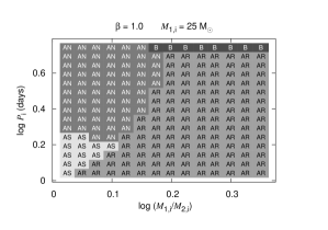
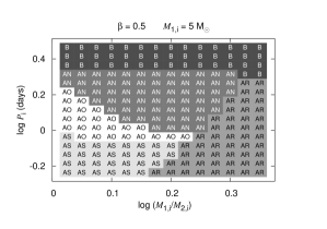
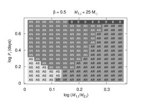
We have calculated four data cubes of binary evolution tracks with different initial primary masses $M_{1,i}$, mass ratios $q_{i}=M_{1,i}/M_{2,i}$ and separations or orbital periods $P_{i}$. The subscript $i$ is used to indicate that these values are the initial values, i.e. at the moment both stars start burning hydrogen on the main sequence. These parameters are spaced at approximately equal logarithmic intervals,

$$\begin{array}[]{cccccc}\log M_{1,i}&=&0.55,&0.60,&\ldots,&1.55,\\ \log q_{i}&=&0.025,&0.050,&\ldots,&0.350,\\ \log(P_{i}/P_{\mathrm{ZAMS}})&=&0.05,&0.1,&\ldots,&0.75,\\ \end{array}$$

with $P_{\rm ZAMS}$ an approximation of the orbital period at which the initially more massive component would fill its Roche lobe on the zero-age main sequence for a system with equal masses,

$$P_{\rm ZAMS}\approx\frac{0.19M_{1,i}+0.47M_{1,i}^{2.33}}{1+1.18M^{2}_{1,i}}.$$ (6)

One data cube of binary tracks is calculated assuming conservative mass transfer $(\beta=1)$. Three additional data cubes are calculated assuming non-conservative mass transfer $(\beta=0.75,0.5\ \mathrm{and}\ 0.25)$. Each binary evolution track is terminated when one of the following conditions is met:

• 4000 time steps are taken,

• The stellar radius exceeds the Roche lobe radius by more than 10%, which happens if deep contact is established, a situation our code is not designed for.

• The mass loss rate becomes larger than $3\times 10^{2}M/\tau_{\mathrm{KH}}$, where $M$ is the mass of the initially more massive star and $\tau_{\mathrm{KH}}$ its Kelvin Helmholtz timescale. These systems are expected to come into contact.

• The code fails to converge. This occurs for example during advanced burning stages and in models for which the mass loss rate becomes very high. These models are expected to come into contact shortly after.

3.1 Subtypes of case A evolution

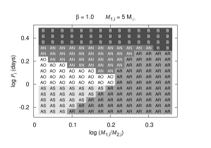
Our conservative grid of models is very similar to the survey of case A binary evolution at solar metallicity published by Nelson & Eggleton (2001). In line with their definitions we identify different subtypes of case A binary evolution. As an example the subtypes are plotted in Figure 1 for two different primary masses and for different assumptions about the mass transfer efficiency $\beta$.

• Case B: In our widest systems the initially most massive star will not fill its Roche lobe before depleting hydrogen in the core. A system is classified as case B if it fills it Roche lobe after leaving the main sequence, which we define as the moment the central hydrogen abundance drops below $0.001$.

• Case AR Contact during rapid mass transfer: In systems with large mass ratios, the mass-accreting star reacts to the mass exchange by expanding rapidly as it is driven out of thermal equilibrium. This leads to a contact situation during the first rapid phase of case A mass transfer. If the mass transfer rate $\dot{M}$ just before contact occurs is larger than $2\%$ of the typical thermal mass transfer rate $M/\tau_{\rm KH}$ a system is classified as case AR.

• Case AS Contact during slow mass transfer: Binaries with small periods and moderately equal masses stay semi-detached during thermal-timescale mass transfer, but come into contact during the subsequent slow nuclear-timescale mass transfer phase.

• Case AO Contact by overtaking: Mass transfer accelerates the evolution of the mass-accreting star. Especially in lower-mass systems there is a significant range of initial separations for which the mass-accreting star depletes its central hydrogen first. Most systems come into contact shortly afterwards as the mass-accreting star expands in the Hertzsprung gap. This subtype corresponds to case AE in Nelson & Eggleton (2001), with the small difference that we explicitly check if the system comes into contact.

• Case AN No contact on the MS: Wider systems with moderately equal mass can avoid contact while both components are still on the main sequence. This subtype comprises cases AG, AL, AN and AB in Nelson & Eggleton (2001) between which we do not distinguish here.

Figure 2: The natural logarithm of the radius over the Roche lobe radius as function of time for the mass-accreting star in binary systems with initial primary mass $M_{1,i}=18M_{\odot}$, initial orbital period $P_{i}=2.2$ days for three different mass ratios. The primary star of the system with $\log q=0.2$ fills its Roche lobe at an age of $\approx 8.87$ Myrs. During the phase of rapid mass transfer the mass-accreting star expands so much that contact is established. Shortly afterwards it restores its thermal equilibrium and shrinks inside its Roche lobe again. The mass-accreting star in the system with $\log q_{i}=0.1$ stays well inside its Roche-lobe. The accreting star in the $\log q_{i}=0.3$ system excess its Roche Lobe by more than 10%. We stop the evolutionary calculations as our code is not able to handle deep contact configurations. Systems with more extreme initial mass ratios are likely to merge during rapid mass transfer.

3.2 Comparison to Nelson & Eggleton (2001)

In contrast to Nelson & Eggleton (2001) our models are calculated at $Z=0.004$ instead of $Z=0.02$. Due to lower opacity the stars are more compact, which causes the different subtypes of case A binary evolution to shift to smaller orbital periods.

Another difference between our survey and Nelson & Eggleton (2001) is that in our version of the code the equations for both stars are solved simultaneously instead of first evolving the primary star, keeping track of the mass transfer rate and then evolving the secondary applying the stored mass transfer rate. This enables us to model reverse mass transfer, although this does not occur often and it is not very relevant for the comparison with observations we undertake. A second advantage is that we continue our evolutionary calculations when the stars reach contact, see Figure 2. Therefore we find a subset of type AR systems that come into contact during rapid mass transfer, but in which the mass-accreting star quickly restores its thermal equilibrium and shrinks inside its Roche lobe again. This is followed by a slow mass-transfer phase like in systems that avoid contact altogether during rapid mass transfer. Some of the observed systems may have followed this type of evolution. Further evolution is either as case AS, AO or AN.

Figure 3: Time in years (color shading) spent in a semi-detached configuration for binary systems with different initial parameters. For a description of the difference between the four diagrams and their axis see Fig. 1. The duration of the semi-detached phase for non-conservative models is longer than for conservative models and more systems avoid contact during rapid mass transfer, see also Fig. 1. This trend is seen for all different primary masses in our grid of binary models over the full range of $\beta$

3.3 The influence of the mass transfer efficiency

An important effect of lowering the mass transfer efficiency is that more systems avoid contact during rapid mass transfer. The critical mass ratio, which defines the border between type AN and type AR systems is up to $25\%$ larger if we assume $\beta=0.5$ than for the conservative tracks, see Fig 1. Since contact during rapid mass transfer potentially has catastrophic consequences for the further evolution of the binary, we expect that non-conservative mass transfer results in a larger number of binaries reaching a long-lived semi-detached phase.

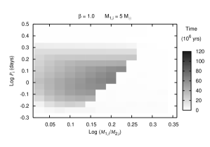
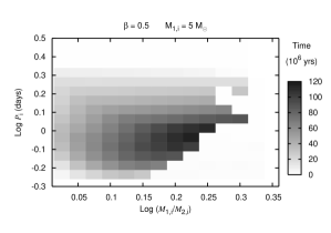
The mass transfer efficiency also strongly influences how much time a binary systems spends in a semi-detached phase, see Fig 3. The accreting star will be less massive in non-conservative models and therefore it will evolve more slowly. The duration of the slow mass transfer phase can be twice as long for non-conservative models ($\beta=0.5$) compared to the conservative models.

The implication of non-conservative mass transfer that more binary systems become semi-detached and the duration of the semi-detached phase is longer, can in principle give a strong test of the mass transfer efficiency if the number of semi-detached systems is compared to the number of detached systems. However, a good understanding of the selection effects and knowledge of the initial mass-ratio distribution are critical in performing such a test.

4 Observed systems

Table 1: Parameters of 50 double-lined eclipsing binaries in the SMC. Details are given in Section 4.

id	OGLE-id	$M_{p}(M_{\odot})$	$M_{p}/M_{s}$	$R_{p}(R_{\odot})$	$R_{s}(R_{\odot})$	$T_{p}(kK)$	$T_{p}/T_{s}$	$P$ (d)
		Detached systems
01	04 056804	$13.0\pm 0.3$	$0.912\pm 0.019$	$4.11\pm 0.09$	$4.94\pm 0.08$	$30.1\pm 2.0$	$1.245\pm 0.017$	1.08987
02	04 103706	$17.5\pm 0.6$	$1.768\pm 0.020$	$5.36\pm 0.13$	$4.05\pm 0.12$	$27.8\pm 2.0$	$1.028\pm 0.017$	1.35585
03	04 163552	$13.3\pm 1.0$	$1.070\pm 0.052$	$5.31\pm 0.15$	$5.18\pm 0.15$	$25.5\pm 2.0$	$1.005\pm 0.007$	1.54581
04	05 038089	$17.1\pm 1.5$	$0.893\pm 0.058$	$6.27\pm 0.21$	$6.19\pm 0.26$	$30.1\pm 2.0$	$1.033\pm 0.036$	2.38946
05	05 095194	$20.3\pm 4.5$	$0.870\pm 0.149$	$8.06\pm 0.56$	$9.53\pm 0.66$	$33.8\pm 2.0$	$1.038\pm 0.002$	3.18742
06	05 140701	$6.9\pm 0.7$	$1.307\pm 0.064$	$7.88\pm 0.31$	$7.01\pm 0.31$	$23.5\pm 2.0$	$1.535\pm 0.025$	3.62544
07	05 180064	$10.7\pm 0.4$	$1.521\pm 0.019$	$5.57\pm 0.27$	$4.49\pm 0.29$	$25.5\pm 2.0$	$1.493\pm 0.107$	2.51491
08	05 255984	$11.6\pm 2.0$	$1.659\pm 0.133$	$4.16\pm 0.43$	$3.38\pm 0.34$	$25.5\pm 2.0$	$1.019\pm 0.038$	1.56384
09	05 305884	$17.6\pm 1.3$	$1.086\pm 0.059$	$7.76\pm 0.27$	$6.52\pm 0.37$	$33.8\pm 2.0$	$1.040\pm 0.007$	2.17648
10	05 311566	$12.9\pm 0.6$	$1.261\pm 0.034$	$4.38\pm 0.13$	$3.21\pm 0.19$	$30.1\pm 2.0$	$1.050\pm 0.024$	3.29139
11	06 011141	$15.1\pm 0.3$	$1.068\pm 0.016$	$5.05\pm 0.05$	$5.01\pm 0.06$	$30.1\pm 2.0$	$1.324\pm 0.027$	1.17737
12	06 180084	$16.2\pm 1.3$	$1.169\pm 0.073$	$5.85\pm 0.25$	$5.70\pm 0.25$	$27.8\pm 2.0$	$0.995\pm 0.011$	1.47523
13	06 215965	$16.0\pm 0.5$	$0.931\pm 0.027$	$9.91\pm 0.19$	$10.35\pm 0.19$	$27.8\pm 2.0$	$1.000\pm 0.037$	3.94304
14	06 221543	$11.9\pm 1.8$	$1.025\pm 0.103$	$5.27\pm 0.48$	$4.53\pm 0.52$	$25.5\pm 2.0$	$0.959\pm 0.009$	3.41678
15	07 120044	$12.5\pm 0.5$	$1.004\pm 0.028$	$4.78\pm 0.10$	$4.68\pm 0.12$	$25.5\pm 2.0$	$0.998\pm 0.016$	1.31081
16	07 255621	$9.3\pm 0.8$	$1.293\pm 0.049$	$5.04\pm 0.29$	$3.54\pm 0.56$	$25.5\pm 2.0$	$1.091\pm 0.043$	4.33063
17	08 087175	$12.0\pm 1.0$	$1.119\pm 0.073$	$4.48\pm 0.21$	$4.38\pm 0.22$	$25.5\pm 2.0$	$1.033\pm 0.021$	1.10226
18	08 104222	$13.1\pm 0.9$	$1.078\pm 0.055$	$5.25\pm 0.38$	$5.19\pm 0.38$	$25.5\pm 2.0$	$1.012\pm 0.033$	1.56384
19	10 037156	$19.5\pm 0.4$	$1.147\pm 0.014$	$7.19\pm 0.16$	$4.41\pm 0.46$	$32.2\pm 2.0$	$1.028\pm 0.012$	2.69834
20	10 110440	$10.8\pm 2.1$	$1.825\pm 0.131$	$3.97\pm 0.39$	$3.66\pm 0.34$	$25.5\pm 2.0$	$1.194\pm 0.027$	1.56384
21	11 057855	$12.4\pm 1.1$	$1.510\pm 0.061$	$5.22\pm 0.21$	$3.73\pm 0.24$	$27.8\pm 2.0$	$1.072\pm 0.039$	1.29695
		Semi-detached systems and contact systems (47 and 49)
22	01 099121	$11.3\pm 0.8$	$1.704\pm 0.048$	$4.97\pm 0.19$	$6.66\pm 0.24$	$27.8\pm 2.0$	$1.758\pm 0.018$	2.45890
23	04 110409	$13.7\pm 0.8$	$1.544\pm 0.046$	$4.34\pm 0.20$	$8.36\pm 0.29$	$25.5\pm 2.0$	$1.660\pm 0.017$	2.97315
24	05 026631	$11.5\pm 0.6$	$1.021\pm 0.039$	$5.12\pm 0.11$	$5.65\pm 0.12$	$25.5\pm 2.0$	$1.489\pm 0.026$	1.41169
25	05 060548	$10.8\pm 0.4$	$1.238\pm 0.027$	$8.39\pm 0.14$	$9.63\pm 0.15$	$30.1\pm 2.0$	$1.722\pm 0.025$	3.63863
26	05 202153	$19.9\pm 1.1$	$1.592\pm 0.036$	$9.53\pm 0.26$	$12.84\pm 0.32$	$32.2\pm 2.0$	$1.374\pm 0.012$	4.60677
27	05 208049	$10.0\pm 0.2$	$2.093\pm 0.014$	$6.62\pm 0.08$	$6.82\pm 0.08$	$25.5\pm 2.0$	$1.791\pm 0.020$	3.02982
28	05 243188	$27.3\pm 1.5$	$1.466\pm 0.041$	$7.29\pm 0.19$	$7.89\pm 0.20$	$35.5\pm 2.0$	$1.104\pm 0.002$	1.87174
29	05 277080	$17.4\pm 0.9$	$1.540\pm 0.036$	$5.05\pm 0.14$	$6.82\pm 0.17$	$25.5\pm 2.0$	$1.607\pm 0.015$	1.93934
30	05 300549	$25.4\pm 1.0$	$1.458\pm 0.027$	$6.35\pm 0.11$	$6.15\pm 0.11$	$30.1\pm 2.0$	$1.879\pm 0.030$	1.33167
31	05 316725	$16.9\pm 1.5$	$1.916\pm 0.048$	$6.13\pm 0.25$	$7.66\pm 0.29$	$33.8\pm 2.0$	$1.072\pm 0.006$	2.55606
32	06 077224	$15.9\pm 1.0$	$1.218\pm 0.049$	$8.93\pm 0.26$	$11.52\pm 0.32$	$32.2\pm 2.0$	$1.253\pm 0.026$	3.82087
33	06 152981	$12.5\pm 0.4$	$1.533\pm 0.018$	$4.94\pm 0.08$	$6.26\pm 0.09$	$25.5\pm 2.0$	$1.268\pm 0.009$	2.00334
34	06 158118	$16.0\pm 0.7$	$2.029\pm 0.023$	$7.61\pm 0.15$	$7.38\pm 0.15$	$29.2\pm 2.0$	$1.589\pm 0.020$	2.57832
35	06 251047	$8.1\pm 0.2$	$1.473\pm 0.016$	$4.62\pm 0.11$	$6.40\pm 0.12$	$23.5\pm 2.0$	$1.738\pm 0.012$	2.51323
36	06 311225	$21.2\pm 0.4$	$1.773\pm 0.012$	$6.55\pm 0.06$	$6.69\pm 0.06$	$30.1\pm 2.0$	$1.282\pm 0.015$	1.84606
37	06 319960	$10.6\pm 0.8$	$1.569\pm 0.057$	$4.47\pm 0.18$	$9.38\pm 0.34$	$25.5\pm 2.0$	$1.567\pm 0.014$	4.05690
38	07 066175	$19.6\pm 1.8$	$1.703\pm 0.059$	$7.88\pm 0.31$	$10.38\pm 0.40$	$32.2\pm 2.0$	$1.271\pm 0.021$	3.62638
39	07 142073	$12.6\pm 1.2$	$2.000\pm 0.053$	$9.57\pm 0.35$	$7.75\pm 0.28$	$30.1\pm 2.0$	$1.435\pm 0.019$	3.18871
40	07 189660	$15.3\pm 1.2$	$1.498\pm 0.046$	$5.35\pm 0.16$	$5.98\pm 0.18$	$25.5\pm 2.0$	$1.510\pm 0.014$	1.66784
41	07 193779	$11.6\pm 1.0$	$1.966\pm 0.053$	$5.79\pm 0.21$	$4.93\pm 0.18$	$25.5\pm 2.0$	$1.486\pm 0.019$	1.67293
42	07 243913	$18.6\pm 1.1$	$1.768\pm 0.034$	$8.23\pm 0.20$	$8.28\pm 0.20$	$32.2\pm 2.0$	$1.242\pm 0.015$	2.63160
43	08 209964	$18.8\pm 0.9$	$1.300\pm 0.031$	$7.67\pm 0.20$	$10.69\pm 0.24$	$36.3\pm 2.0$	$1.371\pm 0.014$	3.31475
44	09 010098	$17.8\pm 1.8$	$1.304\pm 0.075$	$5.08\pm 0.22$	$5.06\pm 0.22$	$33.8\pm 2.0$	$1.062\pm 0.003$	1.11208
45	09 047454	$12.6\pm 2.3$	$1.362\pm 0.107$	$4.20\pm 0.26$	$5.58\pm 0.35$	$27.8\pm 2.0$	$1.644\pm 0.029$	1.57397
46	09 064498	$8.4\pm 0.7$	$3.092\pm 0.044$	$5.40\pm 0.24$	$5.10\pm 0.23$	$25.5\pm 2.0$	$1.496\pm 0.032$	2.63512
47	09 175323	$23.5\pm 1.6$	$1.451\pm 0.041$	$10.16\pm 0.26$	$8.48\pm 0.23$	$39.3\pm 2.0$	$1.021\pm 0.006$	2.20596
48	10 094559	$12.0\pm 1.0$	$1.208\pm 0.065$	$4.68\pm 0.21$	$6.19\pm 0.26$	$30.1\pm 2.0$	$1.262\pm 0.019$	1.75193
49	10 108086	$16.9\pm 1.2$	$1.183\pm 0.057$	$5.67\pm 0.18$	$5.32\pm 0.16$	$33.8\pm 2.0$	$1.130\pm 0.038$	0.88308
50	11 030116	$14.3\pm 1.9$	$1.868\pm 0.086$	$7.42\pm 0.42$	$8.05\pm 0.46$	$27.8\pm 2.0$	$1.368\pm 0.016$	2.95427
		Alternative solutions for system 1 (51) and system 6 (52)
51	04 056804	$16.8\pm 2.1$	$1.724\pm 0.088$	$4.46\pm 0.25$	$4.48\pm 0.25$	$30.1\pm 2.0$	$1.250\pm 0.009$	1.08987
52	05 140701	$7.0\pm 0.7$	$1.307\pm 0.064$	$6.00\pm 0.20$	$8.30\pm 0.30$	$24.3\pm 2.0$	$1.493\pm 0.007$	3.62544

The stellar masses, radii and temperatures of the components of 50 double-lined eclipsing OB-type binaries in the SMC were presented by H03 and H05. In this section we will summarize their work. The systems were initially taken from 1400 eclipsing binaries detected in the Optical Gravitational Lensing Experiment (OGLE) survey. 169 systems were chosen for spectroscopic follow-up observations by selecting systems brighter than $B<16$, to allow a sufficient signal-to-noise ratio, and orbital period $P_{\rm orb}<5$, to ensure adequate phase coverage. About 100 systems had spectroscopic observations obtained near quadrature phases calculated from the adopted photometric ephemeris (Wyrzykowski et al. 2004; Udalski et al. 1998). A spectral disentangling procedure was used to establish the orbital parameters directly, together with the average disentangled spectrum of each binary component. Orbital solutions were determined for a total of 50 systems, and were combined with analysis of the OGLE $I$-band light curves to yield complete astrophysical parameters. The 50 systems are spread over the 10 OGLE fields which cover the central 2.4 square degree area of the Small Magellanic Cloud.

Twenty-one systems are in a detached configuration, two are contact systems. The remaining 27 systems are semi-detached and believed to be undergoing their first phase of mass transfer. In Table 1 the observed stellar parameters are summarized. For two of the detached systems, 1 and 6, alternative semidetached solutions were found after the publication of H05. These are listed as system 51 and 52 respectively.

The light curves show no evidence for departures from circular orbits, except for the following detached systems: 10 ($e=0.063\pm 0.002$), 14 ($e=0.113\pm 0.004$), 16 ($e=0.190\pm 0.006$) and 19 ($e=0.013\pm 0.009$). We can therefore assume that the spin periods of the stars in each system are synchronized with the orbital period. The orbital periods are taken from Wyrzykowski et al. (2004) and Udalski et al. (1998). The mass of the brightest component, the stellar radii, their errors and the temperature of the brightest component are taken directly from H03 and H05. We derived the mass ratio $q=M_{\mathrm{p}}/M_{\mathrm{s}}$ (where $M_{\mathrm{p}}$ is the mass of the primary, i.e. the star eclipsed during the deepest eclipse which is usually the most luminous component, and $M_{\mathrm{s}}$ is the mass of the companion) and its error directly from the radial velocity semi-amplitudes $K_{\mathrm{s}}$ and $K_{\mathrm{p}}$ and their errors, given in the same papers ($q=K_{\mathrm{s}}/K_{\mathrm{p}}$). The three authors independently classified the spectral type of the primary component to determine the effective temperature. They estimate the error on the temperature to be in the order of the difference in temperature between two spectral subtypes An error of 1000 K is given in H03 while an error of 1500 K is given in H05. However, the average temperature difference between spectral subtypes in the range O6-B2 is $\sigma_{T_{\rm eff}}\approx 1800$ K. In addition there are significant uncertainties in the conversion of spectral type to temperature at the metallicity of the SMC. Therefore we decided to adopt an error of $\Delta T_{\rm eff}=2000$ K to allow for some systematic uncertainty. The temperature ratio and its error were determined by H05 and H03 from the $I$-band flux ratio. Unfortunately this band is not very sensitive to temperature for OB stars as it covers the Raleigh-Jeans tail of the spectrum. Nevertheless, the formal errors on the temperature ratio as quoted in Table 1 are often very small. Photometric observations in additional bands or higher resolution spectra would improve the determination of the primary temperature, the temperature ratio and their errors.

5 Fit method

For each system in the observed sample we determine the best fitting binary evolution track using a least-squares fit. Our four fitting parameters are the three initial binary parameters that determine the binary evolution track – the initial primary mass $M_{1,i}$, the initial mass ratio $q_{i}$ and the initial orbital period $P_{i}$ – and the age $t$ of the best fitting model on that track.

There is freedom in the set of observed parameters we can use for fitting. To avoid propagation of errors, we preferentially use observables that are determined directly from the light curve and the spectra. For a proper $\chi^{2}$-test the observables should be independent. In case of the semi-detached systems the radius of the Roche-lobe filling star is determined from the light curve, but it is not independent of the mass ratio and the orbital period. Therefore we cannot use all three observables at the same time. In detached binaries the orbital period does not change significantly during the evolution before the onset of mass transfer. Fitting the period within the tiny observed error is pointless given the much larger uncertainties in the other observables. We therefore choose a definition of $\chi^{2}$ which does not include the orbital period. We do demand that a fit solution matches the period within the accuracy of our grid.

We use the following set of six observed parameters, listed in Table 1: the mass of the most luminous star $\log M_{\mathrm{p}}$, the mass ratio $\log q$, the radius of the most luminous star $\log R_{\mathrm{p}}$, the radius of the companion star $\log R_{\mathrm{s}}$, the temperature of the most luminous star $\log T_{\mathrm{p}}$ and the temperature ratio $\log T_{\mathrm{p}}/T_{\mathrm{s}}$. With six independent observables and four model parameters we have two degrees of freedom ($\nu=2$) when we fit semi-detached systems. In the case of detached systems one of our model parameters, the initial orbital period, is degenerate because stars evolve essentially as if they were single until the onset of mass transfer. In practice we therefore have three model parameters which yields $\nu=3$ for the detached systems.

The cube of models only has discrete values for the model parameters $M_{1,i}$, $q_{i}$ and $P_{i}$. Ideally we want to vary the model parameters continuously, but our grid spacing is not fine enough for some of the more accurately determined observables. Following Nelson & Eggleton (2001) we therefore introduce ‘theoretical errors’ $\sigma_{\rm th}$ to account for the discreteness of the model grid. For the total error $\sigma_{j}$ on the $j$-th observed parameter we add the observational error $\sigma_{\rm obs}$ and the model error $\sigma_{\rm th}$ in quadrature,

$$\sigma_{j}^{2}=\sigma_{\rm obs}^{2}+\sigma_{\rm th}^{2}.$$ (7)

This leads to the following definition of $\chi^{2}$,

$$\chi^{2}\,(M_{1,i},\,q_{i},\,P_{i},\,t\,)=\frac{1}{\nu}\sum_{j}\frac{[\,X_{\mathrm{obs},j}-X_{\mathrm{th},j}\,(\,M_{1,i},\,q_{i},\,P_{i},\,t)\,]^{2}}{\sigma_{j}^{2}}.$$ (8)

The sum is taken over all observed parameters $X_{\mathrm{obs},j}$ and the corresponding values in our models $X_{\mathrm{th},j}$. We determine the best fitting evolution track $(M^{*}_{1,i},\,q^{*}_{i},\,P^{*}_{i})$ and the best fitting age ($t^{*}$) by minimizing $\chi^{2}$ with a systematic grid search of the fitting parameters. We define

$$\chi^{2}_{\min}=\chi^{2}\,(M^{*}_{1,i},\,q^{*}_{i},\,P^{*}_{i},\,t^{*}).$$ (9)

We only allow fit solution in which the observed period is matched within $|\log P_{\mathrm{obs}}-\log P_{\mathrm{th}}|<0.05$. For the theoretical errors we take half the initial grid spacing, i.e. for $\log M_{1,\mathrm{i}}$ and $\log P_{\mathrm{i}}$, $\,\sigma_{\mathrm{th}}=0.025$ and for $\log q_{\mathrm{i}}$, $\sigma_{\mathrm{th}}=0.0125$. We estimate the initial grid spacing for the radii and the effective temperature for each system individually from the two initial models with primary masses closest to the observed mass of the primary.

The initial grid spacing for the logarithm of the temperature ratio scales approximately linearly with the spacing of the logarithm of the mass ratio, with no dependence on the orbital period and a weak dependence on the primary mass. For a typical primary mass of $10\,\mbox{$\mathrm{M}_{\odot}$}$ we fit a straight line through $\log T_{1}/T_{2}$ as function of $\log M_{1}/M_{2}$, which results in an estimate for the theoretical error on the logarithm of the temperature ratio of $0.0065$.

We realize that the introduction of theoretical errors in the definition of $\chi^{2}$ compromises a rigorous statistical interpretation of the obtained $\chi^{2}_{\rm{min}}$ values. Furthermore, using the initial grid spacing is not ideal, especially for post-mass transfer systems, because the real grid spacing will vary during the evolution. Therefore we compared different definitions of $\chi^{2}$ and of $\sigma_{\mathrm{th}}$. We tested the effect of using the orbital period as an observable instead of the radius of the Roche-lobe filling star, and we varied the magnitude of $\sigma_{\mathrm{th}}$ between zero and the full initial grid spacing. The latter definition was used by Nelson & Eggleton (2001). The magnitude $\chi_{\min}^{2}$ for a certain system depends directly the chosen definition; in particular, overestimating $\sigma_{\mathrm{th}}$ leads to artificially low values of $\chi^{2}$. On the other hand, $\sigma_{\mathrm{th}}=0$ can yield artificially high values of $\chi^{2}$ due to incomplete sampling of the model parameters. Therefore, although we attempted to choose a reasonable definition, $\chi^{2}_{\min}$ can not be used as an objective criterion to determine whether a fit is good or bad, only as a relative estimate. Nevertheless, we found that the $\chi_{\min}^{2}$ values obtained with different methods are well correlated; in other words, the relative quality of a fit is independent of the chosen fit method. The best fitting parameters are not sensitive to the chosen definition, i.e. do not vary more than one step in our grid of models except for a few systems for which no good fit could be obtained at all.

For the detached systems we only take detached solutions, i.e. the radii of both stars should be smaller than 98$\%$ of their Roche-lobe radii. This definition is consistent with the definition used for the observed systems (H05). For the semi-detached systems we only accept solutions during which the evolution is slow, on a nuclear timescale. Case A mass transfer starts with a phase of rapid mass transfer on the thermal timescale, $\tau_{\rm KH}$. After the mass ratio reverses, the orbit widens and a phase of slow mass transfer follows on the nuclear timescale, $\tau_{\rm nuc}$, of the mass-donating star. As $\tau_{\rm KH}\approx 0.01\tau_{\rm nuc}$ one would expect only 1 out of 100 systems to be in the rapid mass transfer phase, if no other biases play a role. We therefore assume that all observed semi-detached systems are currently in the slow mass transfer phase, and we only fit models in which:

• the donor star is filling its Roche lobe, such that the radius of the initially more massive star is larger than $98\%$ of the Roche-lobe,

• the stars are in thermal equilibrium, i.e. the thermal luminosity of the mass donor is less than $1\%$ of its total luminosity,

• the mass transfer rate is smaller than $1\%$ of the typical thermal-timescale mass transfer rate of the donor, $M_{\mathrm{D}}/\tau_{1,\rm{KH}}$, and

• the donor star has become less massive than the accreting star, $M_{\mathrm{D}}<M_{\mathrm{A}}$.

To determine confidence limits on the fitted model parameters one has to determine for which values of the parameters the condition $\chi^{2}(M_{i},q_{i},P_{i},t)<\chi^{2}_{\min}+c$ is satisfied, varying each parameter in turn, where $c=1/\nu$ to determine $1\sigma$ boundaries for a proper $\chi^{2}$-test. To compensate for any systematic over- or underestimation of the observational and theoretical errors we take $c=\chi^{2}_{\min}/\nu$. As our model grid is discrete we determine the upper and lower limit on each parameter by the maximum and minimum values for which the condition is satisfied, plus or minus half of the grid spacing for that parameter. To estimate the range of $\beta$ values which fit well for a certain model, we first determine the best fitting model for each of the four assumptions of $\beta$, and the corresponding $\chi^{2}_{\rm{min}}$. To obtain $\chi^{2}_{\rm min}$ as a function of $\beta$ on the full range $0.25\leq\beta\leq 1.0$ we interpolate linearly between the four values. Let $\beta^{*}$ denote the best-fitting value of $\beta$. To estimate the confidence limits on $\beta$ we determine for which values $\chi_{\min}^{2}(\beta)<\chi_{\min}^{2}(\beta^{*})+\chi_{\min}^{2}(\beta^{*})/\nu$.

6 Results

The best fitting model parameters for the detached systems are given in Table 2 and for the semi-detached systems in Table 3.

6.1 Detached Systems

Figure 4: Example of a fit for a detached system. The star-shaped symbols indicate the observed parameters for system 21, the circles (green in on-line version) indicate the best-fitting model. The conservative evolution track of the best-fitting model is plotted in dark gray (red) for the star indicated as the primary, see Table 1, and in lighter gray (blue) for the companion. On the left a Hertzsprung-Russel diagram is given for reference, although we do not use the luminosity as a fit parameter. The error bars on the filled star symbols indicate the error on the primary mass, temperature and radius. In contrast the error bars on the open star symbols indicate the error on the mass ratio, the temperature ratio and the secondary radius. The error bars on the circles indicate the adopted theoretical errors on the same quantities (see Sect. 5), which correspond to half the initial grid spacing of the models.

Table 2: Fit-results for the detached systems: The best fitting initial primary mass $M_{1,i}$, initial mass ratio $q_{\mathrm{i}}=M_{1,{\mathrm{i}}}/M_{2,{\mathrm{i}}}$ and initial orbital period $P_{\mathrm{i}}$ are given together with estimates of the 1$\sigma$ confidence limits (for details see the last paragraph of Section 5). The last two columns give the best fitting age on the best fitting evolution track and, for systems with $\chi^{2}<10$, the evolutionary subtype assuming conservative mass transfer, see Section 3.1. The notation AR $\rightarrow$ … indicates that the best-fitting model experiences a temporary contact phase during rapid mass transfer after which the evolution continues as indicated.

id	$\chi^{2}_{\rm min}$	$M_{1,i}$ ($M_{\odot}$)			$q_{\mathrm{i}}$			$P_{\mathrm{i}}$ (days)			$t$ (Myrs)	case
1	43.0	14.1	-4.7	+4.7	1.05	-0.05	+0.24	1.12	-0.21	+0.18	3.1	-
2	21.8	15.8	-2.5	+5.3	1.58	-0.21	+0.15	1.31	-0.16	+0.32	6.8	-
3	1.2	12.6	-0.7	+0.7	1.06	-0.06	+0.03	1.51	-0.08	+0.29	10.6	AS
4	1.7	17.8	-2.8	+1.0	1.06	-0.06	+0.03	2.18	-0.12	+0.60	6.2	AN
5	1.0	20.0	-1.2	+3.7	1.13	-0.13	+0.02	3.21	-0.39	+0.60	8.1	AN
6	114.0	10.0	-3.3	+27.6	1.06	-0.06	+1.31	3.47	-0.42	+1.20	23.7	-
7	10.7	11.2	-1.8	+3.8	1.49	-0.12	+0.14	2.57	-0.41	+0.59	14.8	-
8	4.5	10.0	-1.6	+3.3	1.33	-0.11	+0.21	1.55	-0.18	+0.40	15.3	AN
9	1.2	20.0	-3.2	+1.1	1.13	-0.04	+0.02	2.27	-0.36	+0.47	6.3	AN
10	2.3	12.6	-0.7	+0.7	1.26	-0.11	+0.04	3.02	-0.17	+0.78	3.9	AN
11	30.9	15.8	-3.9	+5.3	1.18	-0.18	+0.19	1.31	-0.30	+0.20	4.3	-
12	2.0	14.1	-0.8	+2.7	1.05	-0.05	+0.10	1.58	-0.25	+0.27	9.4	AS
13	3.6	17.8	-2.8	+1.0	1.06	-0.06	+0.03	4.34	-0.84	+0.53	10.0	B
14	2.1	11.2	-1.8	+2.1	1.06	-0.06	+0.10	3.63	-0.71	+0.63	12.7	B
15	2.0	12.6	-2.0	+0.7	1.06	-0.06	+0.03	1.20	-0.07	+0.42	8.0	AS
16	0.3	10.0	-0.6	+0.6	1.27	-0.04	+0.11	3.89	-0.22	+0.48	17.1	B
17	0.9	11.2	-0.6	+0.7	1.06	-0.06	+0.10	1.15	-0.18	+0.14	9.7	AS
18	0.9	12.6	-0.7	+0.7	1.06	-0.06	+0.03	1.51	-0.08	+0.39	10.7	AS
19	3.1	17.8	-1.0	+3.3	1.19	-0.10	+0.03	2.44	-0.14	+0.77	7.2	AN
20	3.7	11.2	-1.8	+2.1	1.58	-0.12	+0.15	1.45	-0.08	+0.51	9.6	AR
21	1.4	12.6	-0.7	+0.7	1.42	-0.04	+0.12	1.35	-0.21	+0.16	10.0	AR $\rightarrow$ AS

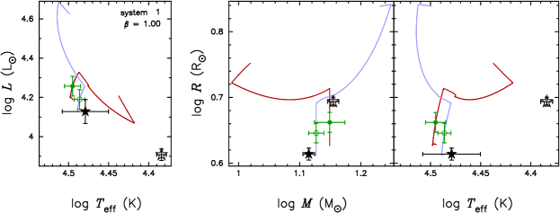
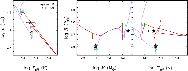
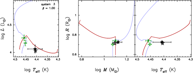
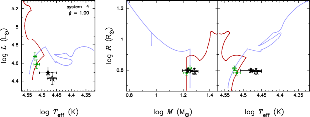
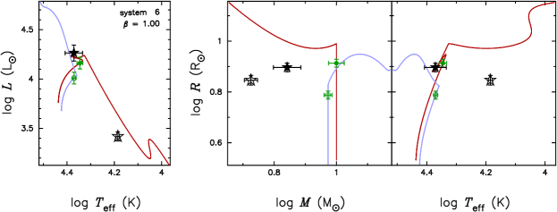
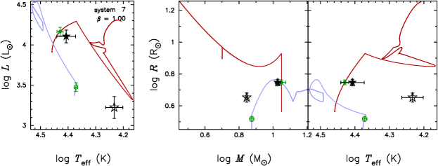
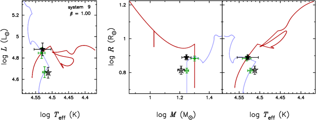
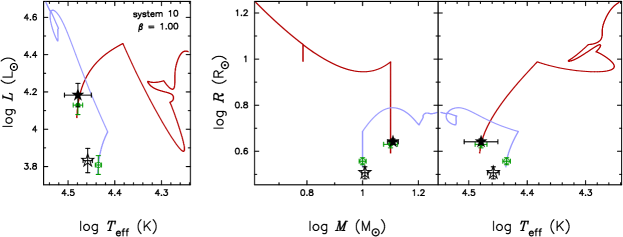
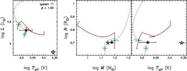
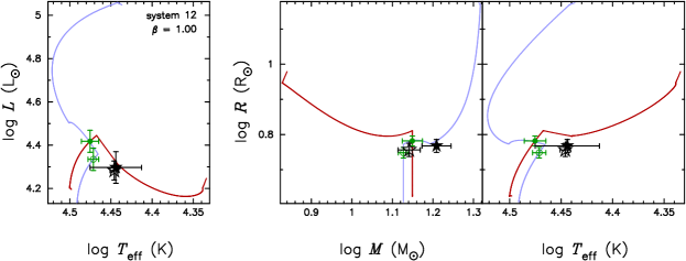
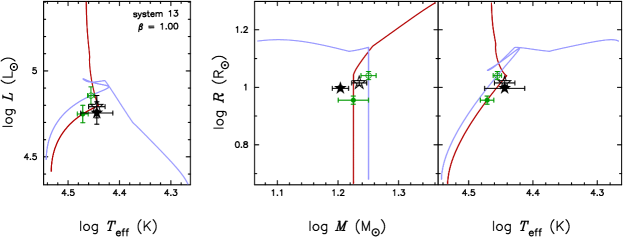
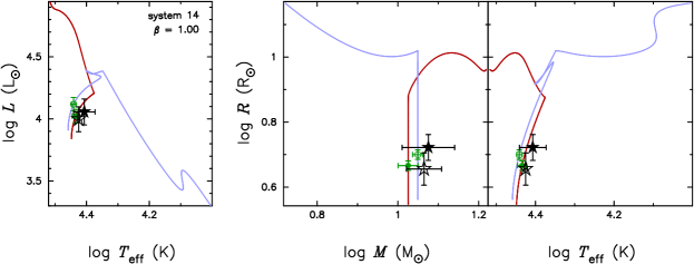
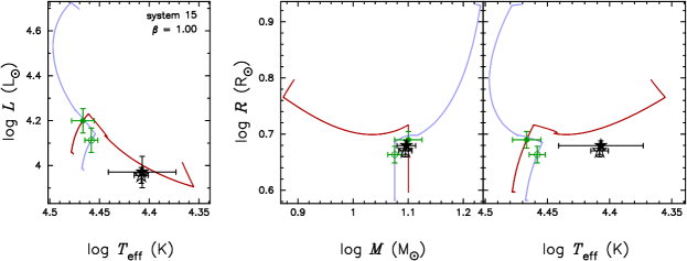
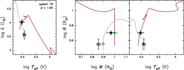
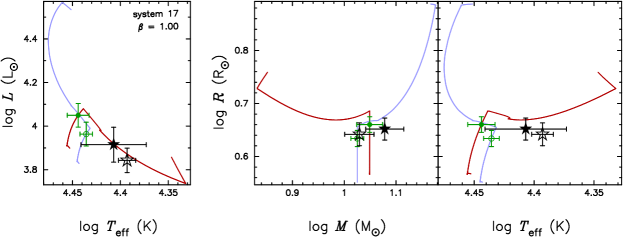
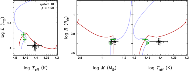
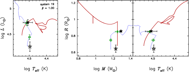
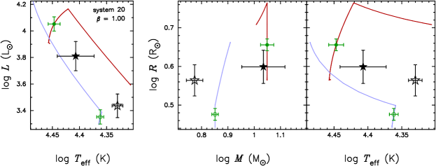
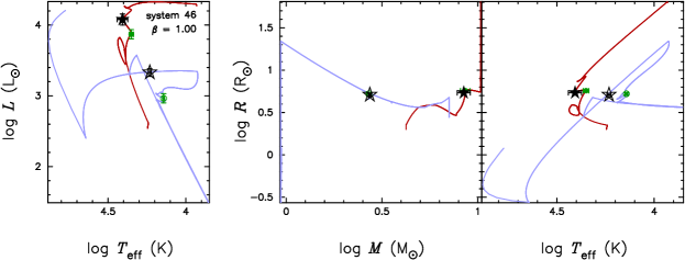
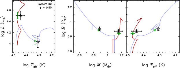
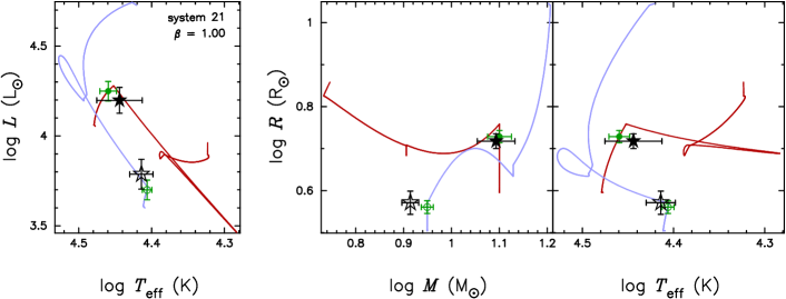
For twelve of the twenty-one detached systems we find good or reasonable fit solutions with a $\mbox{$\chi^{2}_{\rm{min}}$}\leq 3$, see Table 2. Inspection by eye confirms that the fits for these systems are indeed reasonably good, see Figure 4 for an example. An additional set of four systems have $3<\mbox{$\chi^{2}_{\rm{min}}$}<5$, which we still regard as acceptable fits on the basis of eye inspection. For five systems no acceptable fit could be obtained ($\mbox{$\chi^{2}_{\rm{min}}$}>10$). In Sect. 6.1.1 we comment on the individual fit solutions of these systems. Figures similar to Fig. 4 for all systems are given in the on-line Appendix. Here we first discuss the overall properties of the results as presented in Table 2.

If we eliminate system 1 because of the existence of a well fitting alternative semi-detached solution and system 7 because of bad quality of the data (see Sect. 6.1.1) we are left with good or acceptable fits for 16 out of 19 (84%) of the detached systems. We may thus conclude that on the whole our models are able to reproduce the detached binaries in the sample quite well.

In some cases the best fitting solution lies on the border of our grid. This happens often for systems with a mass ratio near 1 as our grid only holds models with initial mass ratios down to 1.059. In two cases the observed orbital period is too high for our grid. This is the case for system 6, for which no good fit could be obtained for other reasons than the period alone, and for system 16 which nevertheless gives a good fit. The boundaries for the masses, the lower boundary for the period and the upper boundary for the mass ratio are never reached.

Out of the 16 systems for which we obtained good or acceptable fits three systems are so wide that our conservative models predict that mass transfer will not start before the most massive star enters the Hertzsprung gap, six systems will start mass transfer on the main sequence but avoid contact, at least until the primary reaches the Hertzsprung gap, and six systems will come into contact during slow mass transfer, see the last column of Table 2. One system will reach contact already during the rapid mass transfer phase.

6.1.1 Comments on individual fits

We first give brief notes on the systems that fit well and then more detailed notes on the systems for which no good fits could be obtained.

Several systems have lower observed temperatures than our models predict: 3, 4, 15 and 18 and to a lesser extent 12 and 17. Good fits with small values of $\chi^{2}_{\rm{min}}$ were nevertheless obtained, because of the large adopted error on the effective temperature of the primary. However, the discrepancy is systematic and the opposite situation does not occur. In addition, the components of system 12 have very equal temperatures, while the masses are different.

Both stars of system 10 are very close to the zero-age main sequence. H05 note that the orbit of this system is slightly eccentric, see Section 4, which is consistent with the young age and the fact that both stars are well inside their Roche lobes. Also systems 14 and 16 have significant eccentricities. Although the stars in these binaries are more evolved than in system 10, both systems have wide orbits and are well detached.

For four systems the fits we obtained were only marginally acceptable, $3\leq\mbox{$\chi^{2}_{\rm{min}}$}\leq 5$:

• For this system we cannot fit the small temperature ratio well at the same time as the moderately large mass ratio, resulting in $\mbox{$\chi^{2}_{\rm{min}}$}=4.5$.

• In this wide and evolved binary, the equal temperatures and the large and almost equal radii of the stars suggest that the masses must also be nearly equal. The best fit ($\mbox{$\chi^{2}_{\rm{min}}$}=3.6$) is obtained with the smallest mass ratio available in our grid, $q=1.06$. We expect that if a model with equal masses were available, we would have found a very good fit for this system.

• The stars in this system have fairly equal masses, while the radii are very different. The less massive component has the size of a zero-age main-sequence star. H05 note that the system may be slightly eccentric. One possibility is that the larger star is still a pre-main sequence star, but this is also the more massive star which should have contracted towards the zero-age main sequence first. Another speculative possibility is that the stars were not born at the same time and that they became part of a binary system after the larger star started burning hydrogen. However, given the moderate value of $\mbox{$\chi^{2}_{\rm{min}}$}=3.1$ such exotic scenarios are probably not required.

• This system has a large secondary radius compared to its mass (the radii are nearly equal whereas the masses are not) which cannot be explained by our detached models. As a result the overall fit is not very good ($\mbox{$\chi^{2}_{\rm{min}}$}=3.7$). An alternative fit solution was found for this system during a post-mass transfer phase. After a rapid phase of mass transfer the donor star briefly detaches when it restores its thermal equilibrium. This alternative fit was not significantly better and the probability of observing a system in the short post-mass transfer phase is small compared to the pre-mass transfer solution.

For five systems no good fit could be obtained:

• This system has nearly equal masses, which is not consistent with the large temperature ratio and the very different radii. The brightest star is the less massive component of the system which fits well to the evolution track of a star that has just arrived on the main sequence. However, the less bright and more massive component is too big and too cool compared to our models.

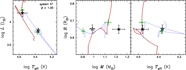
  For this system an alternative semi-detached light curve solution was found. This alternative solution can be fitted well against the semi-detached models with a reduced $\chi^{2}_{\rm{min}}$ of 1.6. We propose to reject the detached solution published in H03 and H05 and adopt the new semi-detached solution indicated as system 51, see Sect. 6.2.

• The mass ratio of the components in this system is large ($M_{\mathrm{p}}/M_{\mathrm{s}}=1.8$) while the $I$-band flux ratio indicates that the effective temperatures of both stars are very similar. The less massive component is consistent with a single star model, while the more massive component is too cool and too small for its mass compared to the models.

• The large radii of both components in this systems suggest that the stars are close to hydrogen exhaustion in the core, at the end of the main sequence or even at the beginning of the Hertzsprung gap. This implies that, if no mass transfer has taken place yet, the masses of the stars must be nearly equal, approximately $6\,\mbox{$\mathrm{M}_{\odot}$}$. However, one would expect approximately equal effective temperatures for both stars, which is not the case. An alternative semi-detached solution is available for this system, but no acceptable fit against semi-detached models was obtained either (see Section 6.2).

• The more massive component of this system can be fitted to the evolution track of a $11\,\mbox{$\mathrm{M}_{\odot}$}$ star, but the less massive component is cooler and bigger than one would expect for its mass. However, the light curve has a very small amplitude (0.06 mag) and is poorly defined due to large scatter (H05). Therefore the light curve solution is not very reliable and this system probably should not have been included in the sample.

• The equal masses of this system together with the extreme temperature ratio make this system difficult to fit. The more massive component is consistent with a single star of about 15 $\mathrm{M}_{\odot}$, but the less massive star is too cool compared to the models.

6.2 Semi-detached Systems

Figure 5: Example of a fit for a semi-detached system. The observed parameters for system 50 are plotted together with the best fitting model assuming a mass transfer efficiency of 0.5. See Fig 4 for description of the symbols. According to the best fitting model this system consisted initially of two stars with masses of about 13 and 12 $\mathrm{M}_{\odot}$ and an orbital period of 1.7 days. The most massive star, which lost about 5 $\mathrm{M}_{\odot}$ by Roche-lobe overflow, is now close to the end of its main sequence. This system will come into contact when the mass donor enters the Hertzsprung gap.

Table 3: Fit-results for semi-detached and contact systems. See the caption of Table 2 for a description.

id	$\chi^{2}_{\rm min}$	$\beta$	$M_{1,i}$ ($M_{\odot}$)			$q_{i}$			$P_{i}$ (days)			$t$ (Myrs)	case
22	16.9	1.00	7.9	-1.3	+1.5	1.06	-0.06	+0.16	1.99	-0.32	+0.22	33.9	-
23	17.4	0.50	10.0	-1.6	+1.9	1.19	-0.19	+0.26	2.46	-0.48	+0.27	23.2	-
24	50.0	0.75	10.0	-3.3	+5.0	1.12	-0.12	+0.33	1.74	-0.58	+0.43	20.6	-
25	97.5	0.25	11.2	-2.8	+7.6	1.06	-0.06	+0.24	2.89	-1.09	+1.04	19.7	-
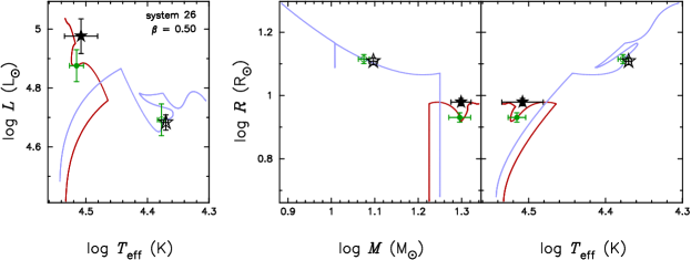
26	4.1	0.50	17.8	-1.0	+3.3	1.06	-0.06	+0.03	3.45	-0.42	+0.36	10.2	AN
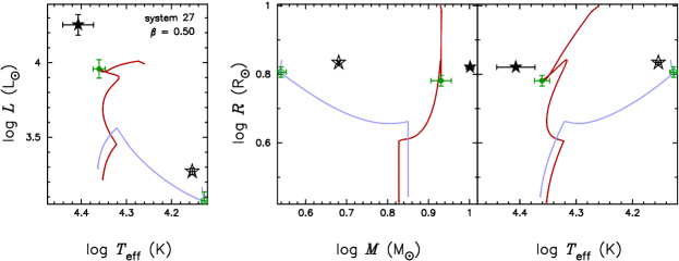
27	26.4	0.50	7.1	-0.4	+2.4	1.05	-0.05	+0.10	1.34	-0.16	+0.87	50.1	-
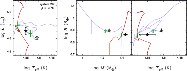
28	1.8	0.75	25.1	-1.4	+4.8	1.33	-0.17	+0.13	1.75	-0.28	+0.18	5.6	AN
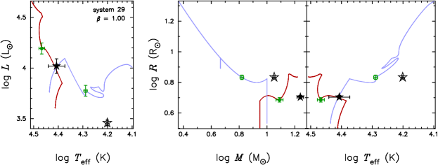
29	31.1	1.00	10.0	-1.6	+3.3	1.12	-0.12	+0.25	1.95	-0.39	+0.59	21.6	-
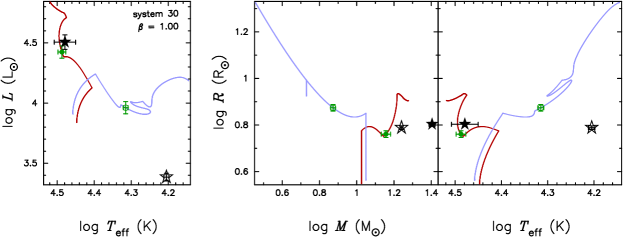
30	141.5	1.00	11.2	-3.7	+7.6	1.06	-0.06	+0.57	2.04	-0.96	+1.08	18.2	-
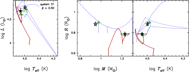
31	1.8	0.50	20.0	-1.2	+1.1	1.69	-0.06	+0.03	2.02	-0.11	+0.12	10.7	AR $\rightarrow$ AN
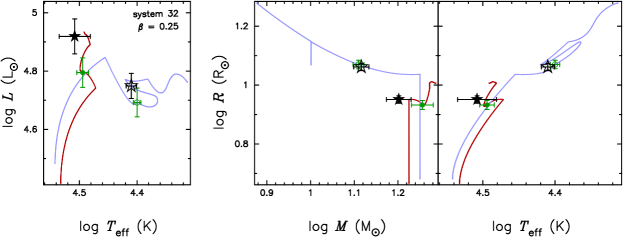
32	5.7	0.25	17.8	-1.0	+3.3	1.06	-0.06	+0.10	3.07	-0.49	+0.32	9.9	AN
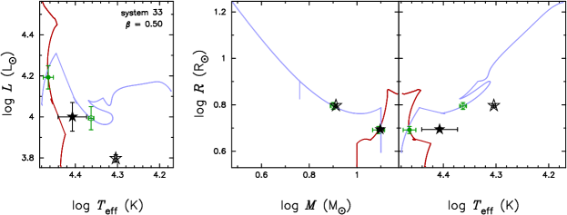
33	1.4	0.50	12.6	-0.7	+0.7	1.26	-0.04	+0.04	1.51	-0.08	+0.09	14.7	AN
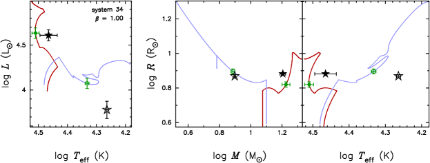
34	15.3	1.00	12.6	-2.0	+2.4	1.06	-0.06	+0.10	1.91	-0.48	+0.36	15.8	-
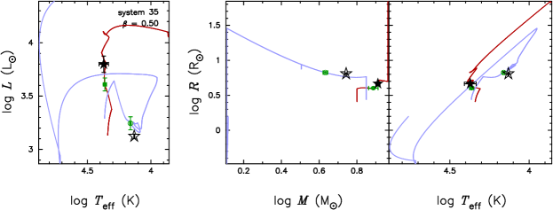
35	41.4	0.50	7.1	-1.8	+2.4	1.12	-0.12	+0.18	1.90	-0.38	+0.47	42.7	-
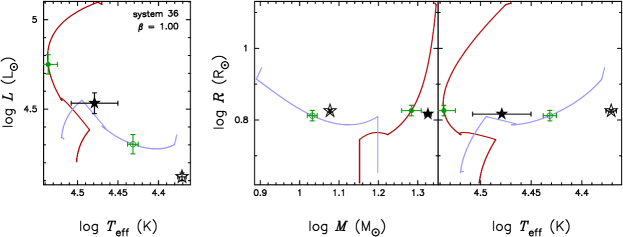
36	3.7	1.00	15.8	-0.8	+3.0	1.11	-0.11	+0.26	1.48	-0.08	+0.28	9.9	AS
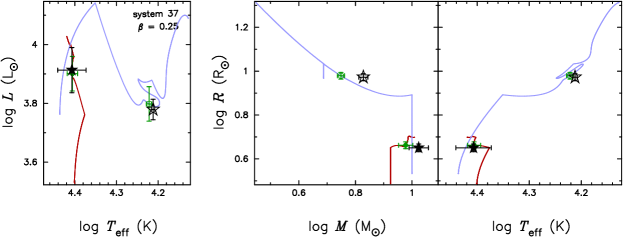
37	3.1	0.25	10.0	-0.6	+0.6	1.19	-0.04	+0.11	2.46	-0.14	+0.15	23.7	AN
38	0.7	0.25	17.8	-1.0	+1.0	1.13	-0.04	+0.03	2.18	-0.12	+0.13	10.5	AN
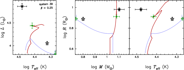
39	10.4	0.25	11.2	-0.6	+2.1	1.06	-0.06	+0.03	1.45	-0.08	+0.27	22.7	-
40	17.7	1.00	10.0	-2.5	+1.9	1.06	-0.06	+0.23	1.95	-0.56	+0.21	21.6	-
41	3.0	1.00	8.9	-1.4	+0.5	1.06	-0.06	+0.09	1.32	-0.21	+0.08	26.9	AO
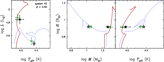
42	0.6	0.50	17.8	-1.0	+1.0	1.06	-0.06	+0.03	1.73	-0.10	+0.10	9.6	AN
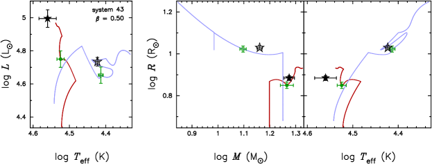
43	14.1	0.50	17.8	-2.8	+3.3	1.13	-0.13	+0.17	2.74	-0.26	+0.66	9.7	-
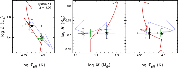
44	1.2	1.00	17.8	-2.8	+1.0	1.19	-0.19	+0.18	1.09	-0.17	+0.06	3.4	AS
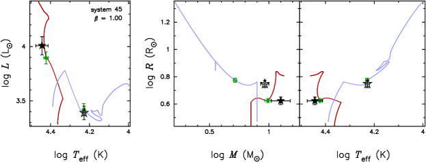
45	11.6	1.00	7.9	-2.0	+2.7	1.12	-0.12	+0.33	1.77	-0.44	+0.29	32.7	-
46	6.5	1.00	7.1	-0.4	+1.3	1.68	-0.22	+0.05	1.34	-0.21	+0.15	63.5	AR $\rightarrow$ AN
47	2.4	0.25	28.2	-1.6	+5.3	1.19	-0.10	+0.11	1.44	-0.08	+0.15	6.1	AS
48	3.5	0.50	11.2	-1.8	+2.1	1.18	-0.09	+0.19	1.82	-0.39	+0.20	17.2	AN
49	0.9	1.00	15.8	-0.8	+1.0	1.05	-0.05	+0.04	1.17	-0.07	+0.07	5.9	AS
50	1.2	0.50	12.6	-0.7	+2.4	1.06	-0.06	+0.03	1.70	-0.09	+0.18	16.3	AN
51	2.6	1.00	12.6	-2.0	+0.7	1.42	-0.19	+0.04	1.07	-0.11	+0.36	12.0	AR $\rightarrow$ AS
52	14.0	0.25	8.9	-1.4	+1.7	1.06	-0.06	+0.09	2.34	-0.46	+0.26	28.4	-

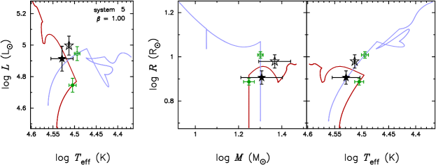
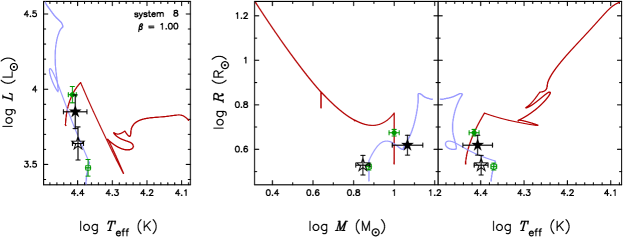
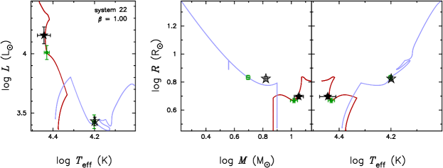
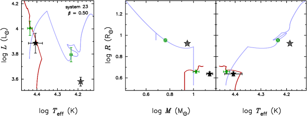
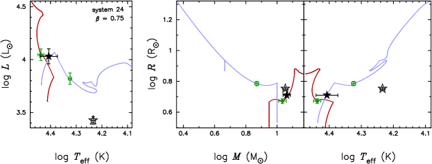
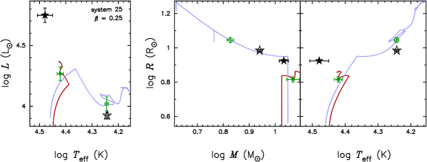
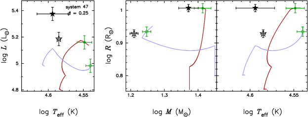
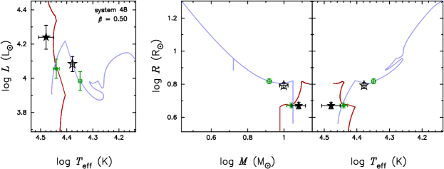
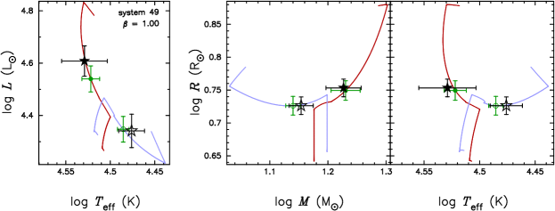
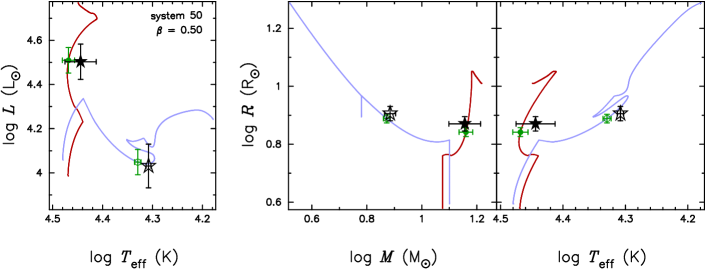
In total there are 29 semi-detached systems and 2 contact systems in the sample, including the two detached systems (system 1 and 6) for which we have alternative semi-detached solutions. The best fitting parameters for these systems are listed in Table 3. An example of a semi-detached system for which we obtained an excellent fit is given in Figure 5.

Our models provide a good or reasonable fit to 11 out of the 31 systems, with $\mbox{$\chi^{2}_{\rm{min}}$}\leq 3$, for at least one value of $\beta$. This includes the two contact binaries. Four systems have $3<\mbox{$\chi^{2}_{\rm{min}}$}<5$, and another two have $\mbox{$\chi^{2}_{\rm{min}}$}\leq 6.5$, and we consider these fits as (marginally) acceptable. The remaining 14 semi-detached systems cannot be fitted well ($\mbox{$\chi^{2}_{\rm{min}}$}>10$). As we have mentioned before the absolute value of $\chi^{2}_{\rm{min}}$ is not a very good measure of the goodness-of-fit. The distinction we make here, and the decision to accept fits with $\mbox{$\chi^{2}_{\rm{min}}$}\leq 6.5$, is primarily guided by eye inspection of the solutions. In Sections 6.2.1 and 6.2.2 we briefly discuss the individual fit solutions, for good or acceptable and bad fits, respectively.

There are several common problems that occur in fitting our models to semi-detached binaries. We distinguish three types of conflicts between the models and the observations:

• q-conflict:   The most ubiquitous discrepancy, occurring in more or less extreme form in all systems with $\mbox{$\chi^{2}_{\rm{min}}$}>5$ except one, is the combination of a relatively small mass ratio (close to unity) with a large or very large temperature ratio. Such a combination cannot be achieved by our models for any value of $\beta$. We discuss possible causes for this problem in Sect. 8.

• R-conflict:   A second discrepancy that plagues nearly half the systems with $\mbox{$\chi^{2}_{\rm{min}}$}>10$, is that the ratio of donor radius over accretor radius, $R_{\mathrm{D}}/R_{\mathrm{A}}$, is smaller than shown by our models, in particular the radius of the accreting star is often under-predicted.

• MT-conflict:   A third problem affecting several systems, is the combination of a large primary mass with a relatively low temperature which cannot be matched simultaneously by our models. The inverse (small mass together with high temperature) also occurs in a few systems.

We refer to these conflicts when discussing the individual systems in Sect. 6.2.2.

The effect of varying the mass transfer efficiency on the fit solutions is often rather obscure, but we can make a number of general statements. The most obvious effect is that lowering $\beta$ results in a smaller (less extreme) post-mass transfer mass ratio, for given initial masses and period and at a given age. The same is true, although somewhat less obvious, for the temperature ratio. Since we are trying to fit a certain observed mass (and temperature) ratio, this means that models with smaller $\beta$ require either a larger (more extreme) initial mass ratio, or a larger amount of mass to be transferred, i.e. a more advanced evolution stage. A consequence of the latter is in many cases a larger donor radius compared to the radius of the accretor. This effect is often (though not always) seen in our best-fitting solutions for a certain system: a smaller $\beta$ leads to a larger ratio of donor to accretor radius, as well as (or sometimes instead of) a less extreme mass ratio.

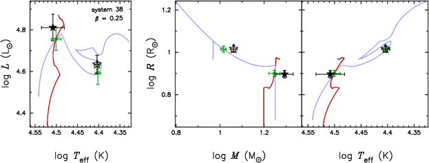
A few systems can be fitted well for different assumptions of $\beta$, such that we cannot determine, on basis of the available observables, if the system has gone through conservative or non-conservative mass transfer. However, in some of these cases (i.e. systems 31, 33, 38 and 51) the surface abundances of carbon and nitrogen differ substantially between the best-fitting models for different $\beta$. This is a consequence of the fact that a smaller $\beta$ yields a fit at a more advanced evolution stage, when the donor star is peeled off to a larger extent. Abundance determinations of carbon and nitrogen would therefore enable us in principle to constrain the mass transfer efficiency. Unfortunately these are not available at this moment, because the resolution of the spectra is not high enough for abundance determinations. We limit ourselves to qualitative statements as the absolute abundances in our models are sensitive to uncertainties in the initial composition and the chemical profile inside the star.

6.2.1 Comments on individual fits: $\mbox{$\chi^{2}_{\rm{min}}$}<6.5$

The seventeen systems for which we found fits that we deem acceptable are discussed individually below. We focus the discussion on the characteristics that distinguish the best-fitting mass transfer efficiencies.

• This is one of the brightest systems, with an O9.5 primary. H03 mention the high quality of the spectra. The asymmetric light curve shows evidence for an accretion stream.

  Our non-conservative models ($\beta\leq 0.5$) give better fits to this system. In fits to conservative models, the primary mass and temperature prefer tracks with small initial masses, but they cannot be fitted at the same time as the mass ratio and accretor radius, which are better explained by models with higher initial masses. The substantial value of $\chi^{2}_{\rm{min}}$ is dominated by the contribution of the accretor radius, which is somewhat under-predicted in all models.

  This is the semi-detached system with the widest orbit, both currently and initially. As a consequence it experienced mass transfer in a late stage of the primary’s main-sequence phase, and the current slow mass-transfer phase will be relatively short.

• This system, consisting of two O stars, is the most massive in the whole sample. It fits well to models with $\beta=0.5-1.0$ and an initial mass ratio of about 1.3, although the effective temperature is overestimated by more than one sigma assuming conservative evolution. According to these models the system is currently seen in the early stages of the slow mass-transfer phase. For $\beta=0.25$ the observed primary mass (which requires a model with an initially massive primary) cannot be fitted well together with the primary radius and the mass ratio, which prefer models with a lower initial primary mass and more extreme mass ratio.

• The best fit to this systems is for $\beta=0.5$ with a large initial mass ratio (1.7). This model narrowly missed contact during rapid mass transfer, and predicts the current system to be near the end of the slow mass-transfer phase, not long before core H-exhaustion of the initial primary. Conservative ($\beta\geq 0.75$) models also require a large initial mass ratio to fit the currently observed one, but fail to account for the observed temperature ratio. These conservative models undergo temporary contact during rapid mass transfer, and it is not excluded that this system evolved fairly conservatively through a deeper temporary contact phase, which we cannot model properly.

  As a result of the advanced evolution stage, our models predict that the C and N abundances have reached equilibrium at the surface but oxygen has not, and the O abundance depends quite strongly on the adopted value of $\beta$.

• This system has a fairly wide orbit, and the components have very similar masses. The only acceptable fit for this binary is for highly non-conservative evolution ($\beta=0.25$). The fit is not very good ($\mbox{$\chi^{2}_{\rm{min}}$}=5.7$) as the models over-predict the mass ratio and under-predict the primary mass, but these problems are much worse for higher mass-transfer efficiencies. It is possible that a value of $\beta<0.25$ would fit this system better.

• This system fits best for $0.5\leq\beta\leq 0.75$, although the best fitting models overestimate the effective temperature by more than 1 sigma. Conservative models overestimate the temperatures even more, whereas models with $\beta=0.25$ under-predict the masses, but these models are not strongly excluded.

  For decreasing values of $\beta$ the best-fitting models start with a more massive primary and a more extreme mass ratio, so that the initial secondary mass is always $\approx 10\,\mbox{$\mathrm{M}_{\odot}$}$. The less conservative models fit this system in a later phase of evolution, when more mass has been transferred. Abundance measurements of C and N could possibly distinguish between a conservative and non-conservative solution, since the predicted model abundances for this system depend quite strongly on $\beta$.

• This system has a fairly large mass ratio. The best-fitting models assume conservative mass transfer $\beta\geq 0.75$. However, the model temperatures are larger than observed while the masses are smaller (a problem that also occurs in many of the poorly-fitting systems, Sect. 6.2.2). The main problem with the non-conservative models is that the masses are under-predicted even more by the models, by about $2\mbox{$\mathrm{M}_{\odot}$}$

• With an orbital period of 4 days, this system is one of the wider systems in the sample. Only very non-conservative models ($\beta<0.5$) can fit both the large radius of the Roche-lobe filling star and the much smaller radius of its companion at the same time as the mass ratio of the system. Like system 26, this binary underwent mass transfer fairly late on the main sequence and the primary is currently close to hydrogen exhaustion in its core.

• This system fits well to non-conservative models ($\beta\leq 0.53$) not long before the donor will leave the main sequence. For the more conservative models, the observed masses and temperatures would fit better against initially less massive models, while the radii and temperature ratio would fit better against more massive models. Also for this system the best-fitting models suggest that abundance measurements of C and N (and perhaps O) could possibly constrain $\beta$ further.

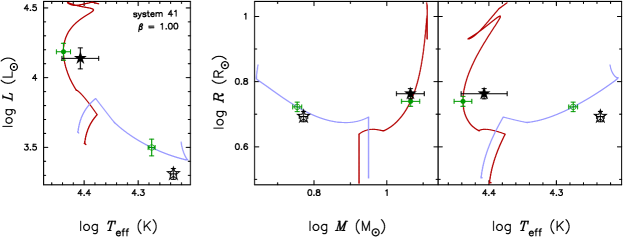
• A good fit to this system, which has a large mass ratio and temperature ratio, is obtained for fairly conservative evolution ($\beta\geq 0.75$), assuming that the system started with a mass ratio near unity. The non-conservative models cannot fit the observed masses (which prefer models with larger initial masses) at the same time as the temperature ratio and the radius of the Roche-lobe filling star.

• This system can be fitted well assuming non-conservative evolution, particularly for $\beta=0.5$. The main problem with fitting a conservative model is the large radius of mass-accreting star (nearly equal to that of its companion) in comparison with its mass and temperature. This system is very similar to system 38 in terms of its inferred initial mass and mass ratio, but started with a smaller period.

• This system is fitted well by our models without a clear preference for a certain mass transfer efficiency. It has one of the shortest periods in the sample, and in all models mass transfer started soon after the onset of hydrogen burning and will eventually lead to contact (case AS evolution). The smaller the value of $\beta$, the closer to contact the system currently is, according to our models.

• This is the least massive of the semi-detached systems and it has the most extreme mass ratio (3.1) of the sample. The non-conservative models cannot explain this extreme mass ratio, to which we obtain the best fit with a completely conservative model with a large initial mass ratio. This model overestimates the temperature ratio, however, and this is the major contribution to the rather poor $\mbox{$\chi^{2}_{\rm{min}}$}=6.5$. The primary temperature is also not perfectly reproduced but the overall fit is acceptable. This model went through a brief contact phase during rapid mass transfer. The Roche-lobe filling star is fitted right at the end of the slow mass transfer phase, and also the accreting star is very close to the end of the main sequence according to this model. The system is on the verge of detaching, before entering another phase of case AB mass transfer.

• This is one of the more massive and hottest systems in the sample, and the light-curve solution indicates it is a near-contact binary in which the primary star fills 99 per cent of its Roche lobe. We find a fairly good fit to a non-conservative ($\beta=0.25$) model in contact, which however somewhat overestimates the masses and underestimates the temperatures. This solution has a very large initial mass of 28 $\mathrm{M}_{\odot}$. For the more conservative models the observed masses, which prefer initially even more massive models, cannot be fitted simultaneously with the other observables.

• This system can be fitted well assuming $0.5\leq\beta\leq 0.75$. More conservative models overestimate the observed small mass ratio. The system is currently seen shortly after the end of the rapid mass transfer phase.

• This is the shortest-period binary in the sample, for which the light-curve solution indicates a deep-contact system. A good fit solution is obtained for all values of $\beta$; only the most non-conservative grid models cannot explain the temperature ratio well. In all best-fitting models the system is still semi-detached but the accreting star is very close to filling its Roche lobe. However, contact is not reached until substantially more mass is transferred.

• The system can be fitted well assuming non-conservative evolution ($\beta\leq 0.5$) and an initial mass ratio near unity. If conservative mass transfer is assumed the primary mass and temperature cannot be fitted well at the same time as the very large radius of the mass-accreting star. On the basis of the best-fitting model we interpret this system as being in the last stage of the slow mass-transfer phase. It is very similar to system 42 in terms of its initial parameters and current evolution state, except for a smaller initial primary mass (and consequently larger age).

• The alternative detached light-curve solution of this system does not fit well to the models, as explained in Sect. 6.1.1. Conservative models with $\beta\geq 0.75$ give good fits to the semi-detached configuration, although the masses are underestimated and the radius of the accreting star is overestimated. This is worse for non-conservative models, which also overestimate the radius of the accreting star. The best fit is found for a model with a large initial mass ratio, which went through a contact phase during rapid mass transfer and is currently undergoing case AB mass transfer. The C/N ratio of the best-fitting models decreases with $\beta$, so that its determination might further constrain the mass transfer efficiency.

6.2.2 Comments on individual fits: $\mbox{$\chi^{2}_{\rm{min}}$}>10$

For the systems, for which we find no acceptable fits, we indicate which of the three common conflicts occur (see the start of this subsection). We divide the systems in two groups, based on their $\chi^{2}$ values. We start with the eight systems that have $10<\mbox{$\chi^{2}_{\rm{min}}$}<20$:

• This system shows the $q$-conflict. Only the conservative models can match the very large temperature ratio of this system, as well as the moderately small value of $R_{\mathrm{D}}/R_{\mathrm{A}}$. The mass ratio is then over-predicted by the models.

• This system exhibits the $q$- and $MT$-conflict. The best fitting model, obtained assuming $\beta=0.5$, fits the observed radii but underestimates the mass of the donor star by about 3 $\mathrm{M}_{\odot}$.

• The $R$-conflict and a moderate form of the $q$-conflict occur for this system. The best fit is obtained with conservative models.

• The $q$- and $R$-conflicts are present as well as a moderate inverse $MT$-conflict.

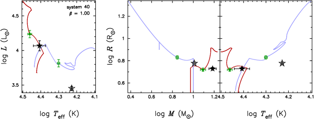
• A combination of all three conflicts occur for this system.

• This system, which shows the $q$-conflict and a moderate inverse $MT$-conflict, has one of the highest effective temperatures. In the best fit, assuming $\beta=0.5$, the temperature ratio is under-predicted and the mass ratio is over-predicted by the models.

• For this system with a $q$-conflict, the conservative models provide a reasonably good fit to nearly all observed parameters for this system except the mass ratio.

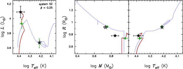
• The alternative detached solution for this model could not be fitted well with our models. The same is the case for the semi-detached solution. The system shows the $q$- and inverse $MT$-conflict. The radius of the accretor is also under-predicted.

Six systems have very poor fit solutions, with $\mbox{$\chi^{2}_{\rm{min}}$}>25$:

• This systems shows a severe form of the $q$-conflict and cannot be matched for any assumption of $\beta$.

• This system suffers from a severe $q$-conflict as well as the $R$-conflict and the inverse $MT$-conflict.

• This system shows the $q$- and $R$-conflict.

• This system exhibits the $q$- and $MT$-conflict.

• This system shows a severe form of the $q$-conflict. The large $\chi^{2}_{\rm{min}}$ is dominated by the contribution of the extreme temperature ratio, which is the largest in the sample. The other two common discrepancies, the $R$- and $MT$-conflict, are also very serious in this system, $R_{\mathrm{D}}/R_{\mathrm{A}}$ is even slightly below unity. The photometric flux ratio is incorrectly reported in H05 as 1.2; it should be 2.7. The spectral type of the secondary component is B2 or later.

• This system is the least massive of all semi-detached systems and cannot be fitted well because of the $q$-conflict.

6.3 Summary of fit results

Figure 6: Fraction of detached (full line) and semi detached systems (dotted line) for which a fit solutions were obtained with $\chi^{2}_{\rm{min}}$lower than a certain value. We have excluded system 1 from the detached systems and system 52 from the semi-detached systems.

As we have argued in Sect. 5, due to the nature of our fit method the absolute value of $\chi^{2}_{\rm{min}}$ is not a very good measure of the goodness-of-fit. The observables we have fitted are not truly independent, and their errors may not in all cases be representative of the true uncertainties. This applies especially to the temperature ratio, which is determined from a flux ratio that is not very sensitive to temperature for OB stars. Also the error on the primary temperature is only a rough estimate. Therefore we feel we can be fairly generous in accepting fit solutions with large $\chi^{2}_{\rm{min}}$, and we have argued in the previous subsections why we regard fits with $\mbox{$\chi^{2}_{\rm{min}}$}\leq 6.5$ as acceptable.

In Fig. 6 we show the cumulative distribution of $\chi^{2}_{\rm{min}}$for the detached and the semi-detached systems. For about $80\%$ of the detached systems and only about $55\%$ of the semi-detached systems we obtain fits with $\mbox{$\chi^{2}_{\rm{min}}$}\leq 6.5$. Interestingly, both distributions show a break between this and larger values of $\chi^{2}$. There is no reason to expect that, if any of the observational errors were underestimated, this should occur preferentially for semi-detached binaries. It is noteworthy that the $q$-conflict, which afflicts a large fraction of the semi-detached fits, only occurs in one detached system (11). We must therefore conclude that our models do significantly worse at explaining post-mass transfer binaries than detached systems which have not yet undergone mass transfer. We will discuss possible causes and the limitations of our models in Sect. 8.

7 Conclusions on the mass transfer efficiency

Table 4: For each semi-detached system $\chi^{2}_{\min}$ is given as function of $\beta$. For each system the value corresponding to the best fitting $\beta$ is marked. The last column indicates the estimated range of $\beta$ which fits well for a certain system.

id	$\beta=1.00$	$0.75$	$0.50$	$0.25$	range
22	16.9∗	18.0	21.3	35.4	0.43$-$ 1.00
23	31.0	22.5	17.4∗	25.9	0.25$-$ 0.86
24	52.3	50.2∗	50.9	57.2	0.25$-$ 1.00
25	142.5	126.0	105.2	97.7∗	0.25$-$ 1.00
26	15.2	6.9	4.1∗	4.2	0.25$-$ 0.69
27	32.9	26.8	26.4∗	28.2	0.25$-$ 1.00
28	2.3	1.9∗	2.4	6.5	0.48$-$ 1.00
29	31.1∗	33.0	41.1	57.1	0.42$-$ 1.00
30	141.4∗	153.8	176.1	212.2	0.25$-$ 1.00
31	22.9	9.6	1.8∗	4.4	0.38$-$ 0.63
32	34.5	22.1	11.6	5.7∗	0.25$-$ 0.38
33	3.2	1.9	1.4∗	3.4	0.38$-$ 0.78
34	15.2∗	15.9	20.2	32.2	0.45$-$ 1.00
35	63.1	43.8	41.4∗	43.1	0.25$-$ 0.99
36	3.7∗	5.1	10.8	27.5	0.73$-$ 1.00
37	30.7	15.0	4.9	3.1∗	0.25$-$ 0.46
38	4.8	2.5	0.8	0.7∗	0.25$-$ 0.53
39	21.5	15.6	12.5	10.6∗	0.25$-$ 0.76
40	17.7∗	19.4	24.1	33.3	0.43$-$ 1.00
41	3.0∗	3.7	7.7	10.4	0.70$-$ 1.00
42	7.4	3.7	0.6∗	2.1	0.38$-$ 0.63
43	28.8	18.2	14.1∗	15.4	0.25$-$ 0.82
44	1.2∗	1.2	1.5	2.1	0.36$-$ 1.00
45	11.5∗	13.3	16.0	22.7	0.45$-$ 1.00
46	6.5∗	8.1	23.6	50.3	0.72$-$ 1.00
47	12.4	7.4	4.7	2.6∗	0.25$-$ 0.38
48	6.8	3.6	3.5∗	5.7	0.31$-$ 0.88
49	0.9∗	1.0	1.2	1.6	0.47$-$ 1.00
50	5.4	3.4	1.2∗	1.4	0.25$-$ 0.63
51	2.6∗	3.3	7.3	14.8	0.72$-$ 1.00
52	42.2	32.3	23.2	14.0∗	0.25$-$ 0.44

Figure 7: The best fitting mass transfer efficiency $\beta$ is plotted against the best fitting initial orbital period $P_{i}$. The symbols indicate the magnitude of $\chi^{2}_{\min}$. The error bars indicate the $1\sigma$ range of the two fit parameters; if the best-fitting $\beta=0.25$ the error bar is extended downward by an arbitrary amount. No strong trend is found but there is a hint that systems with small initial orbital periods evolve more conservatively than wider systems.

Figure 8: As Fig. 7 $\beta$ against mass ratio $q_{i}$.

Figure 9: As Fig. 7 for $\beta$ against primary mass $M_{1,i}$.

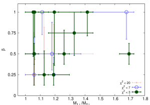
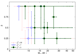
Although a large fraction of the semi-detached systems cannot be fitted well with any assumption for the mass transfer efficiency, we will focus on those systems for which we do obtain reasonable fits to see if we can learn anything about the efficiency of mass transfer from the comparison of models and observations. In Table 4 $\chi^{2}_{\rm{min}}$ is given as a function of the mass transfer efficiency. The last column gives an estimate for the range of $\beta$ for which a certain system can be fitted, as explained in Sect. 5. Some of the semi-detached systems fit significantly better against conservative models ($\beta\geq 0.7$), for example system 36, 41, 46 and 51, while other systems show a strong preference for the non-conservative models ($\beta<0.5$), for example system 32, 37 and 47. There is no single value of $\beta$ for which we can fit all systems. From this we conclude that the simplified assumption of conservative evolution is not valid. Neither is the often made assumption of $\beta=0.5$. Binary systems with different initial parameters cannot be described with one fixed value of $\beta$. The spread in best-fitting $\beta$ values covers the full range of $\beta$.

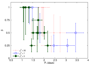
In order to understand the spread in $\beta$, we searched for correlations between the preferred $\beta$ and the initial parameters. In Figure 7 the preferred $\beta$ is plotted against the initial orbital period. The correlation is not strong but there is a region in the upper right part of the diagram where we find no systems: the initially wider systems prefer less conservative models. If real, this correlation might be explained by the interplay of two mechanisms: spin up of the accreting star and tidal interaction. The mass-accreting star is spun up as it accretes angular momentum. Tidal interaction tends to synchronize the stars with the orbit and prevent the accreting star from reaching critical rotation. In wider systems, where tidal interaction is less efficient, the accreting star rotates faster and may lose mass along its equator.

One can expect a strong correlation of the mass transfer efficiency with initial mass ratio, because in systems with extreme mass ratios the accretor will expand rapidly such that a contact system is formed. Mass and angular momentum can than be lost from the outer Lagrangian point. However, we found no correlation of the mass transfer efficiency with the mass ratio in the expected direction, see Figure 8. This might be because the range in current mass ratios available in the sample is small, as the sample is strongly biased towards systems with equal masses. No significant correlation with the initial primary mass was found either, see Figure 9.

8 Discussion

It is striking that we can fit the detached systems in the sample quite well, while a large fraction of the semi-detached systems cannot be explained with our models. We seem to understand the evolution of detached systems well, i.e. essentially the evolution of two single stars, while our models fail to account for a large number of systems in slow mass transfer, especially their temperatures.

In our models we assume a constant mass transfer efficiency throughout the whole evolution. However, mass loss from the system is more likely to occur mainly during the rapid phase of mass transfer. A more realistic description of the mass transfer phases is to be preferred. For instance, spin-up by accretion and associated rotation-induced mass loss can be taken into account, as was done by Wellstein (2001) and Petrovic et al. (2005). However, this treatment introduces other uncertainties, e.g. for the strength of rotation-induced mass loss and the timescale for tidal interaction, which are both uncertain.

For non-conservative evolution we assume that the lost mass carries the specific orbital angular momentum of the accreting star. While the underlying assumption (that the accreting star ejects the surplus of mass isotropically) is reasonable, it may be worthwhile to test the effect of different assumptions. For instance, somewhat stronger angular momentum loss than we have assumed here may improve some of the fits exhibiting the $R$-conflict.

Our models with extreme initial mass ratios show that some systems undergo a temporary contact phase, after which the system restores thermal equilibrium and becomes semi-detached again. A significant fraction of our models with extreme initial mass ratios fail to converge during rapid mass transfer and we stop our calculations if deep contact occurs, as our code contains only a crude model for these contact situations. Improvement of the description of the contact phase might enable us to fit more systems properly.

We assume the Schwarzschild criterion for stability against convection. As a result mass-accreting stars always rejuvenate (i.e. increase the size of their convective core). The question of whether stars rejuvenate or not depends on the still poorly understood efficiency of semi-convection. It is possible that the steep molecular weight gradient, built up before the onset of mass transfer, prevents the star from rejuvenating (Braun & Langer 1995). This shortens the remaining lifetime of the accreting star and affects its position in the H-R diagram as a function of time. Whether this effect would improve any of the fits remains to be investigated.

In principle mass transfer can lead to extra mixing, for example because of spin up and resulting differential rotation, which is not included in our models. If the extra mixing is significant, then chemical abundance profiles in the star will become flatter. In general this results in more compact and therefore hotter stars. As this only affects the mass-accreting star, which is the hotter component, it will lead to more extreme temperature ratios. This might help to solve the discrepancy between the observed and modeled temperature ratios.

To account for the discreteness of our model grid we estimated the spacing in our grid by the initial spacing. The actual grid spacing changes during the evolution and it might even depend on $\beta$. Interpolating between the models would be a solution but this is not simple considering the many dimensions in the grid. We investigated the effect of different values for $\sigma_{\rm th}$ and we found no evidence for systematically under- or overestimating the actual grid spacing for evolved systems.

Our fit method might also be improved by using more directly measured observables. We recall that the most commonly occurring conflicts between our models and the observations are related to the temperature ratio and the radius ratio. For this sample the temperature ratios were derived from the $I$-band flux ratios as determined from the light-curve solution. Rather than fitting to the temperature ratio, we can use the $I$-band flux ratio and its error directly as an observable. The light-curve solution often yields the sum of the radii to a higher accuracy than the ratio of the radii, as a result of which the errors in the individual radii are correlated. It may be preferable to use the sum and the ratio of the radii as observables, rather than the individual radii.

9 Summary and outlook

We computed an extensive grid of detailed binary evolution tracks at a metallicity $Z=0.004$ for a variety of mass transfer efficiencies. Our models are available to the astronomical community. We plan to extend the grid to a larger range of binary parameters and to other metallicities in the future.

We have compared our models to observations of 50 double-lined eclipsing binaries, by fitting evolution tracks to each individual system. For the detached systems in the sample we find generally good agreement between observations and models. Our models can also explain a large fraction of the semi-detached systems although the overall agreement is less good. We identified three common conflicts between the models and the observations.

(I) Several semi-detached systems in which the stars have fairly equal masses are observed to have a large temperature ratio, more extreme (in some cases much more extreme) than our models predict. (II) In some systems the ratio of donor radius to accretor radius, $R_{\mathrm{D}}/R_{\mathrm{A}}$, is smaller than shown by our models, in which case the radius of the accreting star is often under-predicted. (III) A third problem is the combination of a large observed primary mass with a relatively low temperature which cannot be matched simultaneously by our models. The inverse (small mass together with high temperature) also occurs in a few systems.

Conservative mass transfer cannot explain these case A mass transfer systems. We find a large spread in the best fitting mass transfer efficiency. There is no single assumption for $\beta$ which can explain all semi-detached systems. We conclude that the often made assumption of a single constant $\beta$ for all case A binaries is not valid. We find a hint that initially wider systems fit better to non-conservative models. This might indicate the importance of spin up and tidal interaction in determining the efficiency of mass transfer.

We have shown that, assuming non-conservative mass transfer, more systems will avoid contact during rapid mass transfer and that the duration of the slow mass transfer phase becomes longer. This can in principle give a strong test on the mass transfer efficiency by comparing the number of detached and semi-detached systems. Good understanding of the selection effects and the initial mass ratio distribution are needed for such a test.

Although the observed sample we used is currently the largest single set of stellar parameters determined for massive binaries in any galaxy, it is limited in primary masses, mass ratios and orbital periods. It would be interesting to extend this study to all currently known semi-detached double-lined eclipsing binaries in our galaxy and the Magellanic Clouds. This would enable us to study a larger range of primary masses. Studying a larger range of orbital periods and mass ratios will however be difficult as all such samples are biased towards small periods and equal mass ratios.

The largest discrepancies between models and observations are seen in the temperature ratios. The $I$-band flux ratios from which these are determined are not very sensitive to temperature differences as they cover only the Raleigh-Jeans tail of the spectrum. Light curves in the $U$ and $B$-band would lead to more reliable determinations of the temperature ratio. From high quality spectra accurate temperatures can be obtained by fitting model atmospheres.

Our results indicate that surface abundance determinations of nitrogen and carbon can potentially constrain the mass transfer efficiency strongly. If mass transfer is a non-conservative process, then in order to reach a given mass ratio the donor must lose a larger fraction of its mass than for conservative mass transfer. Therefore deeper layers of the star are revealed, in which CN-cycling has increased the N/C ratio. In Section 6.2 we have indicated several particularly interesting and promising targets for further study. In order to determine accurate temperatures and surface abundances, high-resolution spectroscopic follow-up observations are needed.

Figure 10: See Fig 4 for description of the symbols and the units. The observed parameters are plotted together with the best fitting model, see table 2 and 3. For the detached systems we plotted conservative tracks.

Figure 10: Continued.

Figure 10: Continued.

Figure 10: Continued.

Figure 10: Continued.

Figure 10: Continued.

Figure 10: Continued.

Figure 10: Continued.

Figure 10: Continued.

Figure 10: Continued.

Figure 10: Continued.

Figure 10: Continued.

Figure 10: Continued.