Pixelation Effects in Weak Lensing

Abstract

Weak gravitational lensing is a promising probe of dark matter and dark energy requiring accurate measurement of the shapes of faint, distant galaxies. Such measures are hindered by the finite resolution and pixel scale of typical cameras. On the other hand, as imaging telescopes are practically limited to a fixed number of pixels and operational life-span, so the survey area increases with pixel size. We investigate the optimum choice of pixel scale in this trade-off for a space-based mission, using the full engineering model and survey strategy of the proposed SuperNova/Acceleration Probe as an example. Our methodology is to simulate realistic astronomical images of known shear and to evaluate the surface density of sources where the shear is accurately recovered using the Rhodes, Refregier & Groth algorithm in the context of the derived dark matter power spectrum. In addition to considering single exposures, we also examine the benefits of sub-pixel dithering. Although some of our results depend upon the adopted shape measurement method, the relative trends, particularly those involving the surface density of resolved galaxies, are robust. Our approach provides a practical counterpart to studies which consider the effects of pixelation from analytic principles, which necessarily assume an idealized shape measurement method. We find that the statistical error on the mass power spectrum is minimized with a pixel scale equal to $75$–$80\%$ of the FWHM of the point-spread function, and that dithering is marginally beneficial at larger pixel scales.

1 Introduction

The gravitational field arising from a massive foreground structure deflects and distorts the light from distant objects according to the process of gravitational lensing (cf Blandford et al., 1991; Narayan & Bartelmann, 1996). Rapid progress has been made in the accurate measurement of the weakly distorted shapes of background galaxies in order to determine the distribution of dark matter in space and time (for reviews see Mellier, 1999; Bartelmann & Schneider, 2001; Refregier, 2003b). As the growth of the dark matter power spectrum is also sensitive to both the gravitational attraction of dark matter and the repulsive effect of dark energy, weak gravitational lensing is emerging as a very promising cosmological probe (Dark Energy Task Force, Albrecht et al., 2006).

Several proposed space-based missions (SNAP, Aldering et al. 2004; DUNE, Refregier et al. 2006) plan to use weak lensing as a major probe. A key design element is the detector pixel scale, $\theta_{\rm{ccd}}$ (arcseconds), which must be optimized in terms of a trade-off between the fidelity with which the true weak lensing signal is recovered and the benefits of a large survey area during a fixed mission lifetime. In this paper, we investigate the practical consequences of changing the detector pixel scale, using simulations to explore empirically the effect on measurements of the cosmological matter power spectrum.

Extracting the weak lensing signal requires accurate measurements of the shapes of faint galaxies, which are inevitably degraded by the convolutions arising from a finite point spread function (PSF) and detector pixelation. The PSF of an optical space telescope will be dominated by diffraction arising from the system pupils, mirror struts, and other physical structures which perturb incident light. The PSF blurs the shapes of background galaxies, which need to be deconvolved or at least corrected. The shape of the PSF, which typically varies as a function of detector position and time can normally be obtained by examining point sources or directly by ray-tracing software.

Pixelation similarly degrades faint image shapes. In the case of a CCD detector, a photon incident at a photosite, or pixel, photoelectrically liberates an electron, which is then bound near the CCD surface to be measured later. The photosite has finite cross-sectional area and counts photons that fall anywhere inside its perimeter, averaging over all sub-pixel scale image features. Liberated electrons may also diffuse to the surface of adjacent photosites, an effect termed charge diffusion. Averaging and diffusion will distort the measured shape of features nearly the size of a pixel or smaller, biasing the measured weak lensing signal.

While CCD photosites effectively average over small scale image information, it is nonetheless possible to recover some of the high frequency information by dithering. Dithering involves taking multiple exposures of the same stationary objects so that their sub-pixel positions in the CCD are different each time. This can be done by slightly translating the camera between exposures. Individual dithered exposures are combined before shape analysis using the Drizzle algorithm (Fruchter & Hook, 2002) or the Fourier techniques of Lauer (1999a, b); or during shape analysis by somehow averaging the measurements.

The Drizzle algorithm averages dithers on a pixel grid that can be finer than $\theta_{\rm{ccd}}$, resulting in a higher resolution, resampled image. Lauer’s technique accomplishes the same thing without re-pixelation by combining Fourier transforms from the individual dithered exposures. We investigate the extent to which Drizzling can recover weak lensing signals from undersampled data.

Our results are part of a wider investigation of the accuracy of weak lensing measurements and the effects of various instrumental and algorithmic parameters. Our image simulation software is employed by the Shear TEsting Program (STEP). The STEP project comprises independent “blind” analyses of simulated data of various types by international groups with a goal of verifying the limitations of extant weak lensing measurement algorithms. Simulations of both ground (Heymans et al., 2006; Massey et al., 2007b) and space-based (in prep.) data have been undertaken, and in particular space STEP will also explore the effects of pixelation on shear recovery. Bernstein (2002) and Bernstein et al. (in preparation) perform a similar analysis, but starting from the opposite end of analytic first principles, studying the irreversible loss of information during pixelation, even with a perfect shape measurement method. In a further study, Massey et al. (2004b) analyze the effect of varying the exposure time on weak shear recovery from a SNAP-like mission. Refregier et al. (2004) study semi-analytically the trade-off between a wide and deep SNAP survey strategy by looking at the expected errors on cosmological parameters from weak lensing data.

This paper is organized as follows. In §2 we describe a useful mathematical model of pixelation. §3 introduces our adopted PSF model (§3.1) and simulation software (§3.2) and discusses how we vary the pixel scale (§3.3), our simulated dither and Drizzle strategy (§3.4), and our shear measurement algorithm (§3.5). Results are presented in §4. Properties of the simulated images are shown in §4.1, and then the recovered weak lensing signals are analyzed in terms of the surface density of useable galaxies (§4.2), the bias determination (§4.3), the standard error of shear estimation (§4.4), and the predicted error on the matter power spectrum (§4.5). We conclude in §5.

2 A Pixelation Model

Here we introduce the formalism necessary for our analyses. We define the true time-independent image $I^{\rm{tr}}(\boldsymbol{\theta})$ as the monochromatic photon flux at angular location $\boldsymbol{\theta}=(\theta_{x},\theta_{y})$ in the sky, as imaged with a perfect instrument. A real telescope convolves $I^{\rm{tr}}(\boldsymbol{\theta})$ with its “diffraction-pattern” PSF, ${\rm P}(\boldsymbol{\theta})$, which is normalized to unit integral. In our simulations, we take the PSF to be spatially independent across the focal plane.

The PSF-convolved image is then pixelated. Integration within a pixel is equivalent to two distinct operations (Lauer, 1999a, b). First, the PSF-convolved image is again convolved with a pixel response function (PRF) ${\rm R}(\boldsymbol{\theta})$, which has characteristic size $\theta_{\rm{R}}$, producing

$$I^{\prime}(\boldsymbol{\theta})=I^{\rm{tr}}(\boldsymbol{\theta})*{\rm P}(\boldsymbol{\theta})*{\rm R}(\boldsymbol{\theta}),$$ (1)

where $*$ denotes convolution. Second, $I^{\prime}$ is sampled at regular intervals of size $\theta_{\rm{s}}$, such that the observed $ij$-th pixel value is

$$I_{ij}=I^{\prime}(i\theta_{\rm{s}},j\theta_{\rm{s}}),$$ (2)

where $i\in\{1,2,\ldots,N_{x}\}$, $j\in\{1,2,\ldots,N_{y}\}$, and the observed image has $N_{x}\times N_{y}$ pixels.

It is important to emphasize that pixelation is more complicated than a re-sampling of the PSF-convolved image. Photosites integrate photons incident anywhere within their small yet finite borders, allowing only for a spatially averaged, or “binned,” flux measurement. The PRF convolution of Equation [1] fully describes this averaging. CCDs become ideal samplers only in the limit of truly infinitesimal photosites, in which case the PRF is a $\delta$-function and the convolution is simply equivalent to the PSF-convolved image.

The ideal CCD with finite photosite size has a single PRF across the entire array, equal to a unit-normalized square tophat with side $\theta_{\rm{R}}=\theta_{\rm{ccd}}$:

$${\rm R}_{\rm sq}(\boldsymbol{\theta})=\begin{cases}\theta_{\rm{ccd}}^{-2}&\textrm{if $|\theta_{x}|,|\theta_{y}|<\theta_{\rm{ccd}}/2$},\\ 0&\textrm{otherwise}.\end{cases}$$ (3)

Real PRF’s deviate from this idealized case. For example, imperfect quantum efficiency, which results in only a fraction of incident photons being counted, is equivalent to an ${\rm R}$ normalized to less than unity. Similarly, variable quantum efficiency across the array is equivalent to a spatially-varying ${\rm R}$; and charge diffusion can be regarded as a PRF with $\theta_{\rm{R}}>\theta_{\rm{ccd}}$.

We can apply this formalism to consider the performance of single exposures and dithered images (“dithers”) of various kinds. A single exposure is an image $I_{ij}$ with sample spacing $\theta_{\rm{s}}=\theta_{\rm{ccd}}$. A dither refers to the case where the camera is translated by, e.g. non-integral pixels $(d_{x},d_{y})$ delivering an observed image $I_{i-d_{x},j-d_{y}}$, also with $\theta_{\rm{s}}=\theta_{\rm{ccd}}$. Ideal interlacing is a particularly important case consisting of $N\times N$ dithers with $d_{x}=k/N$ and $d_{y}=\ell/N$, where $N$ is a positive integer, and $k,\ell\in\{0,1,\ldots,N-1\}$. Drizzle can deinterlace such dithers, say from half-$\theta_{\rm{ccd}}$ shifts ($N=2$), by applying them to a pixel grid that is twice as fine, yielding an observed image with $\theta_{\rm{s}}=\theta_{\rm{ccd}}/2$. Drizzling in general is an effective “re-pixelation,” with its own PRF that is free to be chosen by the user. We emphasize that the observed image in all cases is convolved with the CCD pixel kernel ${\rm R}$ with size $\theta_{\rm{R}}$, and $\theta_{\rm{R}}\neq\theta_{\rm{ccd}}\neq\theta_{\rm{s}}$ in general. That is, even in the limit of infinite, perfectly deinterlaced dithers with a $\delta$-function re-pixelation kernel, the resultant image is still convolved with ${\rm R}$.

We model the PRF as a square top-hat response convolved with an additional charge diffusion kernel, multiplied by a fraction $\epsilon_{\rm q}\in(0,1]$ representing quantum efficiency. The charge diffusion kernel is taken to be a Gaussian,

$${\rm R}_{\rm ch}(\boldsymbol{\theta})=\frac{1}{2\pi\sigma_{\rm{ch}}^{2}}\exp\left(\frac{\boldsymbol{\theta}^{2}}{2\sigma_{\rm{ch}}^{2}}\right),$$ (4)

where $\sigma_{\rm{ch}}$ is the RMS extent of the diffusion. Our PRF is then

$${\rm R}(\boldsymbol{\theta})=\epsilon_{\rm q}{\rm R}_{\rm sq}(\boldsymbol{\theta})*{\rm R}_{\rm ch}(\boldsymbol{\theta}).$$ (5)

The final size of the PRF, $\theta_{\rm{R}}$, is larger than both $\theta_{\rm{ccd}}$ and $\sigma_{\rm{ch}}$ due to the convolution.

Following Bernstein (2002) and assuming ${\rm P}$ and ${\rm R}$ are both space- and time-invariant, we use the associativity of convolutions to define the effective point-spread function ePSF, equal to ${\rm P}*{\rm R}$. Now $I^{\rm{tr}}(\boldsymbol{\theta})$ is convolved only once, with the ePSF, and then sampled as in Equation 2. Throughout the paper we distinguish between the PSF, ${\rm P}$, which only includes diffraction; the chPSF, equal to ${\rm P}*{\rm R}_{\rm ch}$; and the ePSF, equal to ${\rm P}*{\rm R}_{\rm ch}*{\rm R}_{\rm sq}$.

3 Method

We have developed a pipeline to simulate all relevant steps from the acquisition of imaging data, through its reduction, to the measurement of the weak lensing (or “shear”) signal. We first manufacture realistic images containing galaxies with a known shear signal, with various pixel scales, but keeping all other parameters fixed. We then detect galaxies in the noisy images and measure their shapes. We correct their shapes for ePSF effects, which are measured from separate, simulated images of dense stellar fields at each pixel scale. We finally compare the output, recovered shear measurement to the known input shear signals. In a parallel pipeline, we also create sets of four shallower but dithered images at slightly larger pixel scale, which we stack using Drizzle to improve the pixel sampling. The interlacing of these images is optimal, thus providing an optimistic study of how much resolution could in principle be recovered from a hardware design that slightly undersamples the PSF.

In the following subsections we describe the key ingredients and processes in the pipeline.

3.1 Adopted PSF

The assumption of a constant ePSF in space or time isolates the problem of shear measurement (in which we are primarily interested) without distractions of PSF interpolation (which is a separable problem that is being widely discussed elsewhere).

Our ePSF model is based on an early engineering design, called TMA63, of the SuperNova/Acceleration Probe space telescope (SNAP, Aldering et al., 2004), and accounts for diffraction by the telescope plus charge diffusion in the CCD. The simulated diffraction pattern comes from a raytraced model of the SNAP $f/11$ optical system. It simulates light from an $820{\rm nm}$ wavelength point source incident on a $2{\rm m}$ primary mirror, a secondary supported in front of the primary by three struts, a folding flat, and a tertiary. The point source is taken to be off-axis such that its image appears on the focal plane $198{\rm mm}$ radially away from the optical axis, where the typical SNAP CCD lies. SNAP plans to employ Lawrence Berkeley National Laboratory’s new high resistivity CCDs, in which charge diffusion further spreads point source light (Holland et al., 2003; Stover et al., 2000; Groom et al., 2000). We model charge diffusion as an additional Gaussian convolution with standard deviation $\sigma_{\rm{ch}}=4\micron$, the expected level for these CCDs, which have $10\micron$ wide photosites. The net chPSF has FWHM of $0.12\arcsec$; pixelation at the baseline SNAP CCD pixel scale of $0.10\arcsec$ gives a final ePSF FWHM of $0.14\arcsec$.

3.2 Simulated Images and Input Shear

The image simulation suite of Massey et al. (2004a), Simage, is our main tool for creating artificial astronomical images and applying an arbitrary weak shear signal. Simage uses Shapelets, a parametrization of galaxy morphologies as a weighted sum of a complete, orthonormal set of basis functions (Refregier, 2003a).

Realistic morphologies are generated by empirically matching the measured properties of actual galaxies in the Hubble Deep Fields (HDF, Williams et al., 1996, 1998). The HDF galaxy positions, orientations, morphologies (plus sizes and magnitudes) are randomized when generating new images. In this way realistic magnitude-morphology trends are produced, though no spatial clustering is imposed and no redshift information is encoded . Because the HDF source catalog on which the simulations are based are already pre-convolved with the HDF PSF, they have slightly larger intrinsic sizes than the true galaxy population. However, this does not affect the process of shear addition and measurement.

The analytic shapelet models of galaxies are then sheared as described by Massey & Refregier (2005), including terms up to fourth order in the shear $\boldsymbol{\gamma}$. Our input shears $\boldsymbol{\gamma}=(\gamma_{1},\gamma_{2})$ range from $-0.05$ to $+0.05$ in steps of $0.025$ in each component, while the other component is fixed at $0$, viz:

$$\gamma_{1}\in\{-0.05,-0.025,0,0.025,0.05\}\textrm{ and }\gamma_{2}=0;$$ (6)

$$\gamma_{1}=0\textrm{ and }\gamma_{2}\in\{-0.05,-0.025,0.025,0.05\}.$$ (7)

A total of nine different input shears per pixel scale is thus produced. We make one image per input shear, uniformly distorting all galaxies in the field. The sheared galaxies are convolved with the PSF and transformed to real image space, integrating the basis functions analytically within each pixel. This integration is mathematically identical to the convolution with the ${\rm R}_{\rm sq}$ described in §2. Finally, photon noise and a realistic space background signal are added.

3.3 Pixel Scale

The key question motivating this study is what pixel scale most benefits weak lensing analyses. To address this we simulate and analyze images with CCD pixel scales perturbed about a baseline value chosen to be $\theta_{0}=0.10\arcsec$. In practice, pixel scales can be adjusted in one of two ways and this defines two categories of simulations.

First, we simulate changing the CCD pixel scale $\theta_{\rm{ccd}}$ by changing only the physical size of the photosites, labeling this dataset “Sim 1.” Second, we simulate changing $\theta_{\rm{ccd}}$ by adjusting only the focal length of the telescope, which changes the plate scale, calling this dataset “Sim 2.” While these each linearly perturb $\theta_{\rm{ccd}}$, their detailed effects on the final image are distinct and therefore each merits analysis.

The Sim 1 dataset consists of different simulated images with detector pixel scales between $0.04\arcsec$ and $0.16\arcsec$ at $0.01\arcsec$ intervals. This ranges from the resolution of the processed, end-product HDF images, to just larger than the baseline chPSF size. We adopted a baseline photosite size of $10\micron$, and the different pixel scales are achieved by varying this between $4\micron$ and $16\micron$ in $1\micron$ steps. In practice, such changes would need to be made at the CCD manufacturing stage. Both the diffraction pattern and the baseline plate scale of $0.01\arcsec/\micron$ are unaffected. Thus, assuming the electron diffusion length is constantly $4\micron$ independent of the photosite size, the different photosite sizes cause no net effect in the apparent angular size of the charge diffusion. The final shape and angular size of the chPSF, that is before pixelation, are left unchanged at all $\theta_{\rm{ccd}}$. This scheme for pixel scale adjustment represents a relatively academic exercise into the effect of pixelation of a fixed PSF.

The Sim 2 dataset emulates the effect of changing the focal length while keeping the physical size of the CCD photosite fixed, thereby changing the plate scale and $\theta_{\rm{ccd}}$ from $0.04\arcsec$, to $0.16\arcsec$. At longer focal lengths, the Airy disc from diffraction, which is constant in angular size, grows linearly in microns at the focal plane while the pixel scale decreases in arcseconds and the charge diffusion remains at $4\micron$. At these small pixel scales, the diffraction pattern dominates the chPSF as the first ring is readily apparent. At shorter focal lengths, the Airy disc shrinks while the pixel scale increases. In this case the charge diffusion dominates, smoothing out the diffraction features and broadening the chPSF. This is perhaps a more practical engineering solution to adjusting the pixel scale.

In both cases, the $\theta_{\rm{ccd}}=0.04\arcsec$ images contain $4096\times 4096$ pixels. These dimensions change linearly with $\theta_{\rm{ccd}}$ such that the subtended solid angle per image is constant. This does not necessarily simulate how an instrument would change its CCD array size with $\theta_{\rm{ccd}}$ in practice. We add about $6000$ galaxies and no stars to each sheared image, extending their distribution well below the intended detection threshold. Adding noise to fix the survey depth to $m\simeq 27.7$ with $2000{\rm s}$ exposures, we reproduce the number of galaxies useful for weak shear estimation, $n_{\rm{g}}\approx 100$ per arcmin², found at the baseline pixel scale in earlier studies (Massey et al., 2004b). For each pixel scale, we also make one additional image containing only stars, simulating a weak lensing survey that periodically points at stellar fields to characterize the ch- and ePSF.

Figure 1 illustrates the effect of perturbed CCD pixel scale on the chPSF profile in the two simulation sets.

Figure 1: Cross sections through the peak of the simulated point-spread function on linear (top panel) and log (bottom panel) scales, with components from diffraction and charge diffusion, then finely pixelated at $0.01\arcsec$; this is what we term the chPSF. The baseline chPSF (black line) comes from raytracing simulations of the current SNAP design, convolved with a 2D Gaussian to approximate charge diffusion at the CCD. In this study we perturb the baseline SNAP detector pixel scale of $0.10\arcsec$ in two realistic ways, in parallel, which have distinct effects on the chPSF shape. First, we change only the CCD photosite size in microns, which keeps the angular size of the charge diffusion kernel constant and therefore leaves the pre-pixelated PSF shape unchanged. Second, we adjust only the focal length, which changes the plate scale and thus the angular size of the charge diffusion. In this case, a smaller plate scale reduces the effect of charge diffusion over the diffraction pattern in the final chPSF (light gray line), while a shorter focal length causes the diffraction pattern to dominate (light gray line).

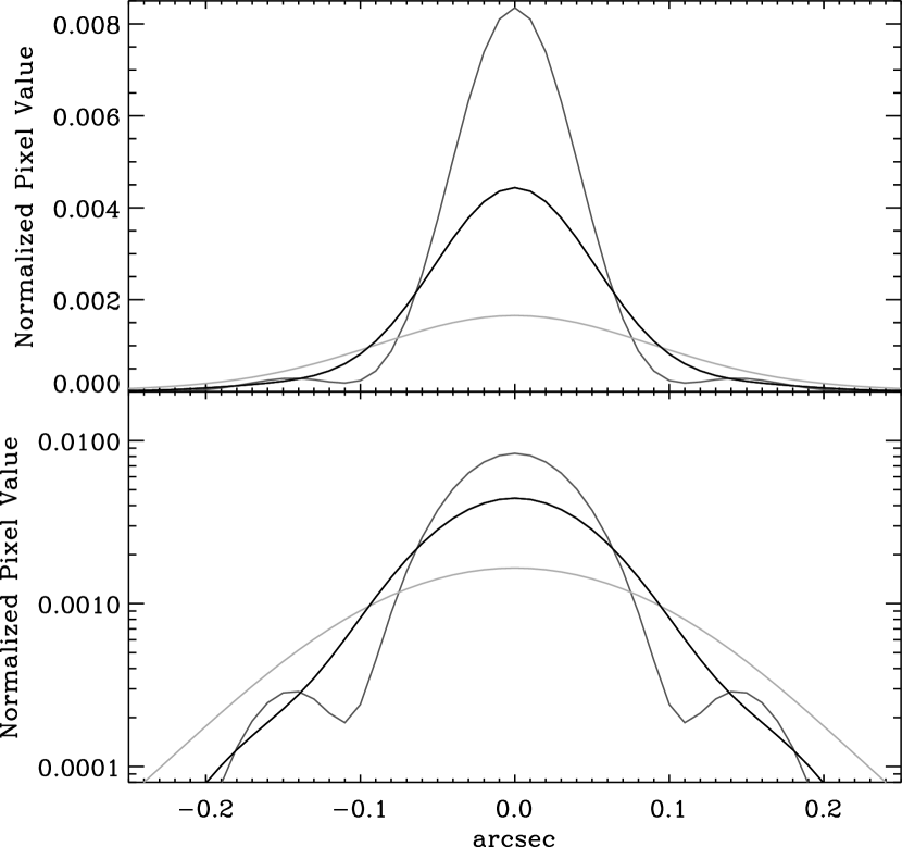
The net result is that the underlying chPSF in all Sim 1 images is constant, while in Sim 2 the chPSF shape and size change with $\theta_{\rm{ccd}}$. Pixelation further distorts the chPSF to produce the ePSF, which we measure and plot in Figure 2.

Figure 2: Measured full-width-at-half-maximum values of the ch- and ePSFs. The chPSF in the Sim 1 (Drizzled) is independent of the CCD pixel scale, while the chPSF in the Sim 2 (Drizzled) increases in angular size with increased $\theta_{\rm{ccd}}$. The plotted chPSF FWHM values (dash lines) are measured from highly oversampled images using Source Extractor. Shapelet coefficients are measured from the oversampled images, and later re-pixelated in the simulated astronomical images at the plotted CCD pixel scales. The ePSF FWHM’s shown are averaged from Source Extracted images containing only stars. The Drizzled images are resampled on pixel grids that are twice as fine as $\theta_{\rm{ccd}}$; we measure stars on the Drizzled images, though we plot their CCD pixel scale values instead to allow comparison with their true underlying chPSFs. As this plot shows, pixelation increases the apparent size of the point-spread function due to the convolution. Drizzling introduces an additional pixelation, which further increases the ePSF size. These effects must be considered in precise shape analyses such as weak lensing requires.

Also plotted in Figure 2 are ePSF sizes after Drizzling, which we discuss presently.

3.4 Simulating and Combining Dithers

In addition to the single exposures introduced above, we also create two additional datasets, labeled “Sim 1 Drizzled” and “Sim 2 Drizzled”, which simulate dithers that we combine to explore the extent to which resolution can be recovered, as described in §1 and §2. Sim 1 Drizzled emulates Sim 1 in how $\theta_{\rm{ccd}}$ varies by changing the size of CCD photosites, and Sim 2 Drizzled emulates how Sim 2 changes the pixel scale by changing the plate scale.

In the Drizzled datasets we implement the simplest, ideally interlaced $2\times 2$ dither pattern, where four exposures are taken, each shifted by exactly half a pixel in orthogonal directions. These dithers resample the ePSF-convolved image from Equation 1 at shifted intevals $(d_{x},d_{y})$, where

Dither 1: $$(d_{x},d_{y})=(0,0)$$ (8)

Dither 2: $$(d_{x},d_{y})=(0.5,0)$$ (9)

Dither 3: $$(d_{x},d_{y})=(0.5,0.5)$$ (10)

Dither 4: $$(d_{x},d_{y})=(0,0.5)$$ (11)

We then deinterlace them using Drizzle, placing the four dithers on a pixel grid that is twice as fine, such that $\theta_{\rm{s}}=\theta_{\rm{ccd}}/2$, and setting Drizzle parameter pixfrac=0.5. We map each dither pixel to one Drizzled pixel with no overlap, such that the noise between adjacent pixels is uncorrelated. Note that this is an idealized case, impossible to achieve in practice, and therefore represents an optimistic case study.

All dithers and Drizzled images subtend the same solid angle as in the other two studies. Each dither is a $500{\rm s}$ exposure, resulting in a $2000{\rm s}$ effective exposure after Drizzling. The CCD pixel scale $\theta_{\rm{ccd}}$ varies from $0.08\arcsec$ to $0.24\arcsec$ in steps of $0.02\arcsec$, so the final Drizzled pixel sampling scales, $\theta_{\rm{s}}$, range from $0.04\arcsec$ to $0.12\arcsec$. Table 1 summarizes the four simulation sets .

Table 1: Summary of the simulations.

Sim Set	Perturbation	Plate Scale	$\sigma_{\rm{ch}}$	$\theta_{\rm{s}}$
Sim 1	Photosite size in $\micron$	$10\arcsec{\rm mm}^{-1}$	$4\micron=0.04\arcsec$	$\theta_{\rm{ccd}}$
Sim 1 Drizzled				$\theta_{\rm{ccd}}/2$
Sim 2	Focal length (plate scale)	$10\arcsec{\rm mm}^{-1}\times\frac{\theta_{\rm{ccd}}}{\theta_{0}}$	$4\micron=0.04\arcsec\times\frac{\theta_{\rm{ccd}}}{\theta_{0}}$	$\theta_{\rm{ccd}}$
Sim 2 Drizzled				$\theta_{\rm{ccd}}/2$

3.5 Weak Lensing Measurement

We now turn to exploiting the simulated images in order to recover the weak lensing signal and thereby determine the surface density of useable galaxies under various assumed pixel sizes and exposure strategies.

We locate galaxies in the noisy images using Source Extractor (Bertin & Arnouts, 1996) configured to detect all objects as near to the noise threshold as possible via a Gaussian detection kernel matched to the known size of the chPSF at each pixel scale. The size of the detection kernels are therefore proportional to the chPSF FWHM values plotted in Figure 2. Source Extractor convolves the images with this detection kernel, blurring features smaller than the size of the kernel, such as pixel-to-pixel photon counting noise, to avoid spurious detections.

We adopted the shear measurement method by Rhodes, Refregier, & Groth (2000, hereafter RRG) to measure the shapes of detected galaxies. RRG was specifically developed with space-based weak lensing measurements in mind (Rhodes et al., 2000) and has undergone extensive tests on simulations (Leauthaud et al., 2007) and use on Hubble Space Telescope images (Rhodes et al., 2001; Refregier et al., 2002; Rhodes et al., 2004; Massey et al., 2007a) to constrain cosmological parameters including $\sigma_{8}$, the normalization of the dark matter power spectrum.

RRG is a modification of the KSB+ (Kaiser et al., 1995; Hoekstra et al., 1998) method which measures Gaussian-weighted multipole image moments,

$$J_{ij}=\int~{}{\rm d}^{2}\boldsymbol{\theta}w(\theta)I(\boldsymbol{\theta})\theta_{i}\theta_{j},$$ (12)

where $w$ is a Gaussian; $i,j\in\{x,y\}$, corresponding to the orthogonal image coordinates; and $\boldsymbol{\theta}$ is chosen such that the weighted barycenter is zero. RRG corrects the galaxy image moments for ePSF effects using the moments of the measured ePSF. More advanced shape-measurement algorithms that are being developed, including the Shapelets-based method of Massey et al. (2007), instead model the chPSF. This requires higher resolution data, but allows information known a priori about a regular pixel response function to be included analytically, whether that be a fixed ${\rm R}_{\rm sq}$ or known pixel-to-pixel variations in the PRF.

RRG forms a measure of ellipticity (in contrast to KSB+), only at the final stage, after correction of individual shape moments

$$\boldsymbol{e}=\frac{(J_{xx}-J_{yy},2J_{xy})}{J_{xx}+J_{yy}}.$$ (13)

A shear estimator is then formed,

$$\hat{\boldsymbol{\gamma}}=\frac{\boldsymbol{e}}{G},$$ (14)

where the shear susceptibility $G$ is a scalar function of higher order moments of the ensemble of galaxies.

We then remove objects from the shear catalog in a similar manner to analyses of real data by Massey et al. (2007a); Leauthaud et al. (2007), and shown by the dashed lines in figure 5. We first eliminate the $<1\%$ of galaxies that Source Extractor misclassified as stars, and also use the Source Extactor $\rm{s/n}$ outputs flux_auto and fluxerr_auto to cut galaxies with $\rm{s/n}<10$.

We then calculate the ‘RRG size’, defined using the uncorrected quadrupole image moments as

$$d_{\rm{rrg}}=\sqrt{\frac{J_{xx}+J_{yy}}{2}}.$$ (15)

We remove large galaxies with $d_{\rm{rrg}}>2000$, which eliminates fewer than $1$ detected object per arcmin² in our simulations. And via

$$d_{\rm{rrg}}<1.2\sqrt{d_{*}^{2}+0.4}\equiv d_{\rm{cut}}.$$ (16)

we eliminate galaxies whose size is nearly equal to the measured ePSF. The $0.4$ term also eliminates galaxies that are only a few pixels across, which have $d_{\rm{rrg}}\approx 1$. This term is negligible at small pixel scales, as Figure 3 shows, because the ePSF is large in pixel units.

Figure 3: Lower size limit $d_{\rm{cut}}$ in pixels (solid, left axis) and arsec (dash, right axis) vs $\theta_{\rm{ccd}}$. (Note the left axis doesn’t map horizontally to the right axis since $\theta_{\rm{ccd}}$ is made to vary.) $d_{*}$ is the median $d_{\rm{rrg}}$ measured on high $\rm{s/n}$ stars at each $\theta_{\rm{ccd}}$. This study applies cuts with the $0.4$ term, which has miminal effect at small $\theta_{\rm{ccd}}$, but causes the size limit to tend toward about one pixel (dotted line) at large pixel scales. Plotted here are cuts made in the Sim 2 study, with size cuts in other simulation sets behaving similarly.

At large $\theta_{\rm{ccd}}$, where the ePSF size is nearly one pixel, the $0.4$ term causes $d_{\rm{cut}}\to 1$ pixel, also seen in Figure 3. This cut ensures we measure shear on galaxies that are somewhat larger than both the PSF and the pixel size, which is the regime shape measurement is most reliable. The effect of the lower size cut on the data is shown with the dashed line below the ellipticity cut in Figure 5. We also test applying a lower size limit of $d_{\rm{cut}}=1.2d_{*}$ instead of Equation 16. This leaves $n_{\rm{g}}(\theta_{\rm{ccd}}\lesssim\theta_{0})$ unchanged within a few galaxies per arcmin² at most, but $n_{\rm{g}}(\theta_{\rm{ccd}}>\theta_{0})$ increases by up to $\sim 10/$arcmin². The result that smaller pixel scales always yield more galaxies, however, is robust.

4 Results

After discussing some properties of the simulated images, we explore as a function of pixel scale: the number of detected and “useful” galaxies for weak lensing measurements $n_{\rm{g}}$; the performance of shear recovery; the sample variance of shear estimators; and the predicted errors on the dark matter power spectrum. The number of galaxies for which shear can be measured is mainly a function of the angular size of galaxies relative to the size of the PSF. These results are therefore likely to be independent of our adopted shear measurement method. However, the performance of shear recovery and the error on the power spectrum will depend upon the sophistication of the chosen method, so those results are likely to improve before the launch of any future space-based mission.

4.1 Image Properties

As an illustration, Figure 4 shows the size and magnitude distributions of galaxies useful for lensing measurements in images from Sim 1 at the baseline pixel scale.

Figure 4: Surface density of galaxies as a function of magnitude (left panel) and size (right panel). These are the galaxies we use to measure the shear, which survive various cuts as described in §4.2, in Sim 1 images with $\theta_{\rm{ccd}}=\theta_{0}$ (black) and $\theta_{\rm{ccd}}=0.4\theta_{0}$ (dark gray), and in Sim 1 Drizzled images with $\theta_{\rm{ccd}}=2\theta_{0}$ (light gray). Magnitude bins are $0.25$ wide, and size bins are $0.05$ wide in $\log_{10}$ space. Magnitude is taken from the Source Extractor mag_auto output, and FWHM from the fwhm_image output.

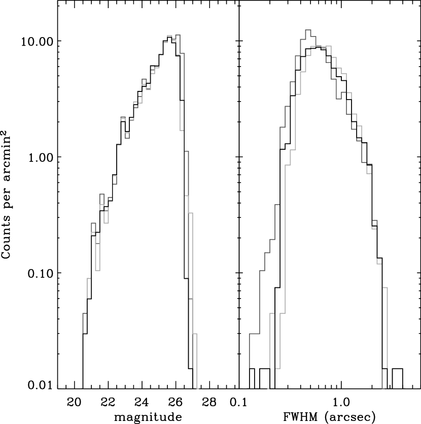
The ordinate axis units are counts per arcmin², and the data are measured on galaxies after we make cuts, as described in §4.2. Our images have a depth of about mag $27.7$, but the faintest galaxies are not ultimately used.

4.2 Surface Density of Sheared Galaxies

The surface density of galaxies that survive the various cuts discussed above is plotted as the solid line in Figure 5. The uppermost dashed lines in each simulation set show the raw galaxy detections using Source Extractor, averaged from all nine sheared images at each pixel scale in each Sim set. The surface density of galaxies that survive this cut are plotted in the next highest dashed line for each Sim set in Figure 5.

Figure 5: The surface density of galaxies detected and usable for weak lensing, $n_{\rm{g}}$, along with counts after different cuts are applied to the data in turn, vs the pixel scale of the reduced images, $\theta_{\rm{s}}$. The top panel plots data from Sim 1 (black lines) and Sim 1 Drizzled (gray lines), and the bottom panel similarly for Sim 2 and Sim 2 Drizzled. Galaxies are detected with Source Extractor, and cuts are made based on measured ellipticity (“e cut”), size (“d cut,” see Equations 15 and 16), and $\rm{s/n}$ (final cut, giving “usable” galaxies). Error bars are calculated as the sample variance of $n_{\rm{g}}$ between the different images at a given pixel scale.

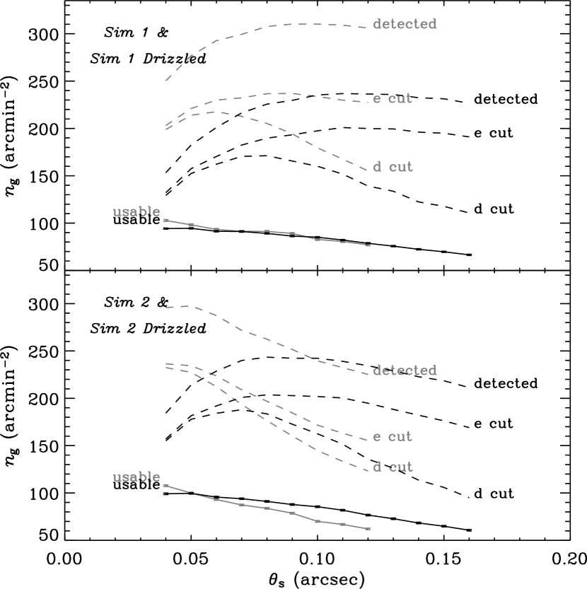
As expected, the usable $n_{\rm{g}}$ decreases monotonically in all simulation sets, indicating that smaller $\theta_{\rm{ccd}}$ always helps decrease counting noise in mean shear measurement for a fixed survey area. Stacking sub-pixel dithers fully recovers the surface density of galaxies from Sim 1, despite larger the CCD pixel convolution at pixel scale $\theta_{\rm{ccd}}=2\theta_{\rm{s}}$. Some galaxies are lost in the Sim 2 Drizzled data. Here the constituent dithers, unlike the Sim 1 sets, have a larger underlying chPSF than the non-stacked counterparts. Taken together, these results indicate that $n_{\rm{g}}$ worsens with increased charge diffusion, but is independent of the CCD pixel spacing $\theta_{\rm{ccd}}$.

We estimate errors on the surface density of usable galaxies, plotted with error bars in Figure 5, to be the sample variance of $n_{\rm{g}}$ measurements between each of the nine simulations per pixel scale. Errors are of order one galaxy per arcmin² for all data, which we consider to be negligible in our analysis.

4.3 Accuracy of Weak Shear Recovery

Figure 6 illustrates the accuracy with which we recover shear measurement with RRG for one typical set of simulated images.

Figure 6: Example of known, input shear vs measured shear, for one set of simulated images. Points are $\langle\hat{\boldsymbol{\gamma}_{i}}\rangle$, measured from the data. Error bars are the standard error of shear estimators in each image. The dotted lines have slope $1$, representing perfect shear recovery, and the solid lines are linear least-squares fits to the data points. Also shown are the $y$-intercept $a$ divided by the standard error of $a$, ${\rm SE}(a)$, and the slope $b$ plus or minus the standard error of $b$, $\rm{SE}(b)$—all outputs from the least-squares algorithm. Also shown are the $\chi^{2}$ values of the fit, which has 7 degrees of freedom.

We define ‘accuracy’ to be the closeness of the measured value to that originally input. In all cases, the shear recovery is well-fit by a linear model thereby justifying the catalog cuts described in §3.5. Relaxing the cuts and using smaller or fainter objects introduces systematic effects that cannot be corrected with RRG. Again in all cases, the $y$-intercepts (“additive shear residual”) of the shear recovery are consistent with zero and accordingly set explicitly so in subsequent analyses.

On the other hand, the best-fit slopes (“multiplicative shear bias”) are systematically smaller than unity by roughly $20\%$. This effect has been known for some time as a limitation of KSB+ methods (eg Bacon et al., 2001; Heymans et al., 2006; Massey et al., 2007b), and it has been speculated to arise as a result of pixelation. The population bias has appeared to be robust to effects like galaxy morphological type, and we assume in all subsequent sections that it could, in practice, be determined to arbitrary accuracy using simulations. We therefore take

$$\boldsymbol{b}\equiv\frac{\rm{bias}}{\boldsymbol{\gamma}}+1,$$ (17)

where, conventionally,

$$\rm{bias}\equiv\langle\hat{\boldsymbol{\gamma}}\rangle-\boldsymbol{\gamma}.$$ (18)

to be the true value with negligible error, and correct for the bias using values from the line fitted as a function of pixel scale in figure 7. We call $\boldsymbol{b}$ the bias for brevity.

Figure 7: The RRG shear estimator bias $\boldsymbol{b}$, and deviation from the least-squares line fitted to each component $\Delta b$, as a function of pixel scale $\theta_{\rm{ccd}}$. Squars indicate the $\gamma_{1}$ component of shear, relative to the pixel grid, and diamonds the $\gamma_{2}$ component. Error bars show the standard error on slope measurement obtained from the least-squares fits to data like those show in figure 6. The bias in each component of shear is different, and varies with pixel scales. Extrapolating the pixel scale to zero appears to give a bias of about $0.8$, so pixelation is likely not the cause of the bias. Drizzling to smaller pixel scales does not remove the bias or the trend toward $0.8$.

4.4 Precision of Weak Shear Recovery

Weak lensing induces changes of only a few percent in galaxy ellipticities, but the RMS of the ellipticity distribution of faint galaxy populations are about $30\%$, (e.g. Leauthaud et al., 2007). Figure 8 shows the standard deviation of ellipticities $\sigma_{e}$ and shear estimators $\sigma_{\gamma}$, where $\sigma_{e}$ is defined analogously to

$$\sigma_{\gamma}^{2}=\sigma_{\gamma_{1}}^{2}+\sigma_{\gamma_{2}}^{2},$$ (19)

where

$$\sigma_{\gamma_{i}}^{2}=\langle(\hat{\gamma}_{i}-\langle\hat{\gamma}_{i}\rangle)^{2}\rangle.$$ (20)

Figure 8: RMS galaxy shapes in single exposure (black lines) and Drizzled (gray lines) simulations. The RMS of the shear is calculated as $\sigma_{\gamma}=\sqrt{\sigma_{\gamma_{1}}^{2}+\sigma_{\gamma_{2}}^{2}}$, where $\sigma_{\gamma i}$ is the RMS of the bias-corrected shear estimators. Errors are calculated as the sample variance of the RMS shapes between different images at a given pixel scale. The RMS of the galaxy ellipticities are calculated similarly from uncorrected ellipticities.

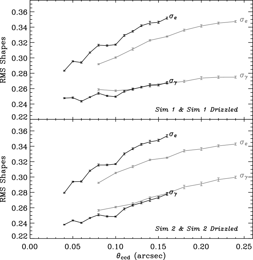
The measured RMS ellipticity increases monotonically with $\theta_{\rm{ccd}}$, meaning larger pixels always make shape measurements noisier, an undesirable effect for weak lensing analysis. The ePSF “dilutes” the shear signal in galaxies, and RRG is shown here to reverse this dilution at all pixel scales by decreasing the RMS of shapes, as expected. The near coincidence of the non-Drizzled and Drizzled $\sigma_{\gamma}$ lines suggests that the RMS shear depends most on the CCD pixel spacing $\theta_{\rm{ccd}}$, and whether or not ideal deinterlacing is performed. This is, in fact, the ideal situation: the best image resolution we can have is fundamentally limited by (in addition to the diffraction) the CCD pixel response—that is, the ePSF. Ideal deinterlacing increases the sample rate of a given object, which is why $\sigma_{e}$ decreases when Drizzling. This plot shows that RRG recovers the underlying, chPSF convolved shape information from the ensemble even without Drizzling.

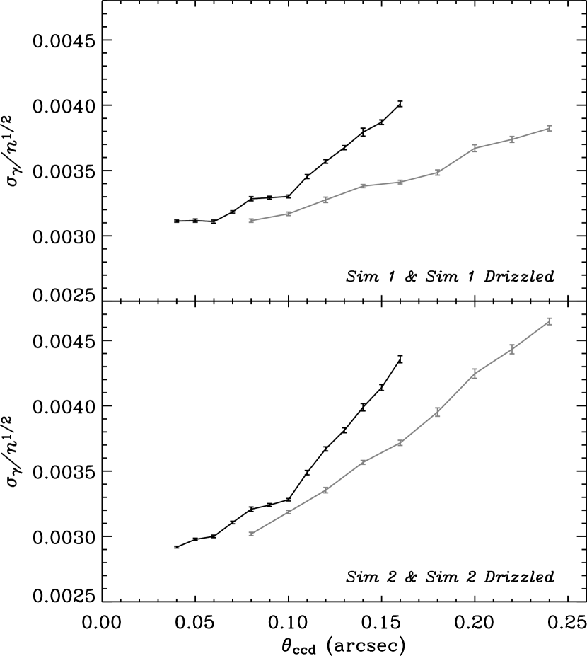
By assuming uncorrelated shapes in galaxy populations (for a discussion, see Hirata & Seljak, 2004), this noise can be reduced by measuring many galaxies and applying Poisson statistics. An ability to use more galaxies per arcmin², $n_{\rm{g}}$, improves the precision of shear recovery, which is best quantified by the sample variance of shear estimators, or its square root $\sigma_{\gamma}/\sqrt{n}$. This is shown as a function of pixel scale in Figure 9. This reiterates our result that smaller pixel scales always improve the precision of weak shear estimation. However, smaller pixel scale face diminishing returns: the loss of precision when increasing the pixel scale by some amount is greater in magnitude than the gain in precision of decreasing the pixel scale by the same amount. Drizzling decreases the error somewhat, thanks entirely to the behavior of $n_{\rm{g}}$ with $\theta_{\rm{ccd}}$. The shear errors from the Sim 2 sets degrade faster with increased $\theta_{\rm{ccd}}$. This indicates that charge diffusion, which dominates larger $\theta_{\rm{ccd}}$ in the Sim 2 sets, should be minimized in addition to $\theta_{\rm{ccd}}$.

Figure 9: The standard error of the shear, $\sigma_{\gamma}/\sqrt{n}$ in the single exposure (black lines) and Drizzled (gray lines) simulations. Error bars are calculated as the sample variance of the standard error between the different images at a given pixel scale. This quantity combines the method-independent $n_{\rm{g}}$ and the more method-dependent $\sigma_{\gamma}$ into an estimate of the precision of our shear estimation. This is the figure of merit showing how precisely we can measure shear as a function of $\theta_{\rm{ccd}}$, if the survey area is fixed.

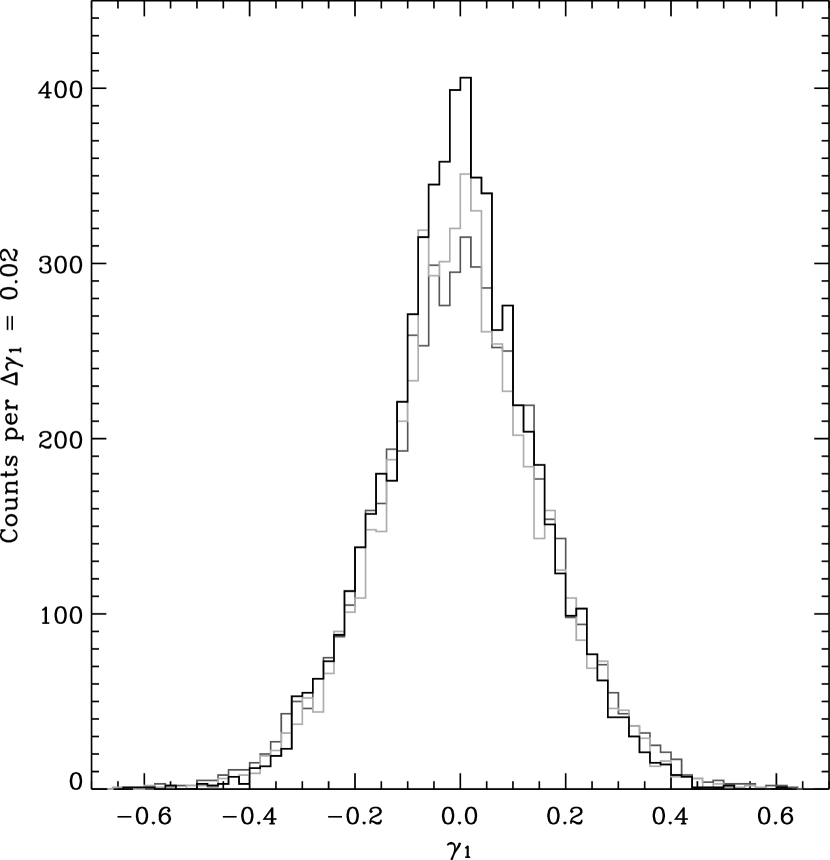
One potential concern is the observation by Kaiser (2000) that the distribution of shear estimators in practice is not Gaussian, and that its extended wings may even make its second moment infinite. This is not surprising because the shear estimator involves a ratio of two noisy quantities. Figure 10 shows the distribution of RRG shear estimators measured in all $9$ images at different pixel scales, and Figure 11 shows the kurtosis of those distributions. The distributions are indeed non-Gaussian. However, there does not appear to be any significant degradation in this sense at larger pixel scales. The skewness of the distributions is also consistent with zero at all pixel scales.

Figure 10: The distribution of shear estimators $\hat{\gamma}_{1}$ obtained from Sim 1 images with $\theta_{\rm{ccd}}=0.10\arcsec$ (black) and $\theta_{\rm{ccd}}=0.04\arcsec$ (dark gray), and Sim 1 Drizzled images with $\theta_{\rm{ccd}}=0.20\arcsec$ (light gray) pixel scales. Each sample comes from all images at the quoted pixel scales, which have different input shears applied. The mean of the input shears at each pixel scale, however, is zero, so these distributions are themselves centered around zero.

Figure 11: Kurtosis of shear estimators minus $3$ as a function of pixel scale. The kurtosis is calculated as $\langle(\hat{\gamma}_{i}-\langle\hat{\gamma}_{i}\rangle)^{4}\rangle/\sigma_{\gamma_{i}}^{2}$, where $\sigma_{\gamma_{i}}$ is the variance of $\hat{\gamma}_{i}$. The $\hat{\gamma}_{i}$ are measured from all $9$ images at each $\theta_{\rm{ccd}}$. $3$ is the kurtosis of a Gaussian distribution. All data here are greater than $0$, showing that the distribution of measured shear estimators has a sharper peak and more extended wings than a Gaussian.

4.5 Cosmological Implications

As we have already seen, the quality of shear measurements is always improved with small pixel scales. However, for a mission with a fixed lifetime, larger pixels would allow a linear increase in the total survey volume, and a corresponding decrease in sample (or “cosmic”) variance errors. These two effects combine in a measurement of the dark matter power spectrum from cosmic shear, which would have a total statistical error (cf Refregier et al., 2004)

$$\Delta C_{\ell}=\sqrt{\frac{2}{(2\ell+1)f_{\rm{sky}}}}\left(C_{\ell}+\frac{\sigma_{\gamma}^{2}}{2n_{\rm{g}}}\right),$$ (21)

where $C_{\ell}$ is the power, and $\ell$ is a multipole. The fraction of sky surveyed is

$$f_{\rm{sky}}(\theta_{\rm{ccd}})=f_{0}\frac{\theta_{\rm{ccd}}^{2}}{\theta_{0}^{2}},$$ (22)

where $f_{0}$ is the baseline fraction, $\theta_{0}$ the baseline pixel scale, and $f_{\rm{sky}}$ at the largest simulated pixel scale is assumed to be still smaller than the observable sky. This introduces a tension between weak lensing precision and cosmic variance. We use the overall error $\Delta C_{\ell}$ as our final figure of merit.

Figure 12: The contribution of shear sample variance to the predicted error on the matter power spectrum in single exposure (black lines) and Drizzled (gray lines) simulations. This assumes the number of pixels in the focal plane is fixed when perturbing $\theta_{\rm{ccd}}$, such that the survey area scales as in Equation (22). The ordinate axis scale is $\log_{10}$, normalized to the Sim 1 error value at the baseline pixel scale, $\theta_{\rm{ccd}}=0.10\arcsec$.

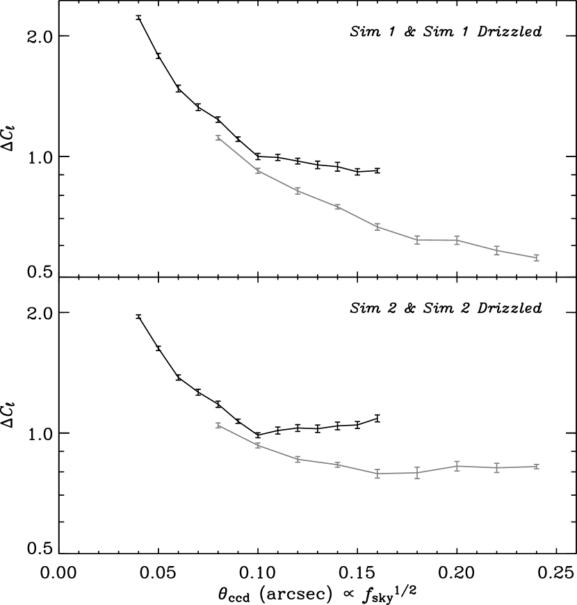
The measured values of the second term (i.e. in the limit of small $C_{\ell}$) are shown in Figure 12. The ordinate axis uses a logarithmic scale, in units of the baseline survey because the absolute values are heavily dependent on the the survey area, multipole $\ell$, number of galaxies, etc. Cosmic variance dominates errors at small $\theta_{\rm{ccd}}$, and increased sample variance in shear estimators takes effect at large $\theta_{\rm{ccd}}$. The error flattens out at larger pixel scales, affording some freedom in choose the pixel scale, in which case the smaller pixel scales are clearly preferred for reasons of caution.

Our idealized Drizzling decreases the error, thanks entirely to the behavior of $n_{\rm{g}}$ with $\theta_{\rm{ccd}}$, indicating larger CCD pixel scales are acceptable if perfect deinterlacing is possible and charge diffusion remains fixed. It is important to note that larger $\theta_{\rm{ccd}}$ degrades $n_{\rm{g}}$, RMS shapes, and ultimately shear errors. As expected, charge diffusion dominates large at $\theta_{\rm{ccd}}$ in Sim 2 sets.

Increasing the survey lifetime while fixing the depth would increase the nominal survey area $f_{0}$, and thus shifts all curves down uniformly on a $\log_{10}$ scale; however, this may increase the range of angular scales probed ($\ell$) and thus change the overall behavior of Equation (21) with $\theta_{\rm{ccd}}$.

5 Discussion

To explore the effects of pixelation on galaxy shape measurement, we have realistically simulated weakly sheared galaxies at a range of pixel scales. We have examined two different ways in which a future weak lensing space mission could alter the pixel scale, and both non-dithered and dithered exposure strategies, for a total of four different simulation sets. We have then emulated the process of shear measurement that is applied to real data. We have finally combined the observed surface density of galaxies, statistics of the shear estimators, and our privileged knowledge of the true input signal, to arrive at figures of merit for the pixel scale.

We find that, as expected, smaller pixel scales consistently give improve the quality of shear recovery and tighten constraints on the dark matter power spectrum for a hypothetical survey of fixed area. Ideal deinterlacing gives a further improvement. On the other hand, when the survey area is permitted to change with the pixel scale according to larger or smaller detectors, we find that larger pixel scales minimize statistical errors on the measured matter power spectrum because the survey area increases as $\theta_{\rm{ccd}}^{2}$. These errors flatten out somewhat above $\theta_{\rm{ccd}}=0.09\arcsec$. Considering both situations of fixed and variable survey area, the best $\theta_{\rm{ccd}}$ would be the smallest allowable by the projected dark matter constraints, which we find to be about $0.75$–$0.80$ the FWHM of the charge diffusion convolved diffraction pattern, chPSF.

We used a current-generation shear measurement method as the basis of our study—a snapshot of available technology. Better methods are certainly needed to fully exploit the ambitious future surveys now being planned. We can speculate that these may either be better able to cope with poor resolution, or (more likely, since information is irrevocably lost during pixelation) require smaller pixels to overcome systematic floors revealed by the lowering of statistical errors. This is being suggested by the variable bias in current results, which is now well documented but poorly understood. It even has to be argued whether the best use of an expensive space mission would be to minimize statistical errors on an isolated measurement of the matter power spectrum. By imaging a smaller region, but with a higher density of useable galaxies, and smaller errors, a mission could alternatively be used to obtain the phase information needed for maps or for higher order correlation functions; or even to calibrate the shape measurement of larger, ground-based surveys. As shown by our results, this approach would prefer smaller pixel scales.

Two important simplifications were imposed on our pipeline. Firstly, we allowed no temporal or spatial variation in the PSF, and a created a comfortably large number of fake stars to characterize the PSF shape. As demonstrated in Rhodes et al. (2007), pixelation especially adds noise to peaky objects like a diffraction-limited PSF. A typical survey region is likely to lie at high galactic latitude. If sufficiently bright stars cannot be imaged within the time taken for the PSF to vary, noise in the measurement of PSF shapes (which we have not considered) could potentially dominate that in galaxy shapes. Secondly, real dither strategies never provide perfect interlacing. For example, optical distortions differentially alter the spacing of the pixel grid in different places, effectively causing $\theta_{\rm{ccd}}$ to be a function of position in the focal plane. Consequently, Drizzling real images correlates noise between adjacent pixels because it must average nearby pixel values. Correlated noise hinders both object detection and shape measurement, so Drizzling is detrimental to weak lensing. The dithering implemented here is therefore idealized, and provides a best-case scenario.

With these caveats in mind, our approach has provided a practical analysis that is achievable with existing methodology. It is complementary to studies starting from analytic first principles and assuming the existence of a perfect shape measurement method. In practice, our result on the optimum pixel scale should sensibly be considered as an upper limit, pending future developments in shape measurement methodology.

References

- Albrecht et al. (2006) Albrecht, A., et al. 2006, astro-ph/0609591
- Aldering et al. (2004) Aldering, G., et al. 2004, PASP, submitted (astro-ph/0405232)
- Bacon et al. (2001) Bacon, D. J., Refregier, A., Clowe, D., & Ellis, R. S. 2001, MNRAS, 325, 1065
- Bartelmann & Schneider (2001) Bartelmann, M., & Schneider, P. 2001, Phys. Rep., 340, 291
- Bernstein (2002) Bernstein, G. 2002, PASP, 114, 98
- Bertin & Arnouts (1996) Bertin, E., & Arnouts, S. 1996, A&AS, 117, 393
- Blandford et al. (1991) Blandford, R. D., Saust, A. B., Brainerd, T. G., & Villumsen, J. V. 1991, MNRAS, 251, 600
- Fruchter & Hook (2002) Fruchter, A. S., & Hook, R. N. 2002, PASP, 114, 144
- Groom et al. (2000) Groom, D. E., Holland, S. E., Levi, M. E., Palaio, N. P., Perlmutter, S., Stover, R. J., & Wei, M. 2000, Nuclear Instruments and Methods in Physics Research A, 442, 216
- Heymans et al. (2006) Heymans, C., et al. 2006, MNRAS, 368, 1323
- Hirata & Seljak (2004) Hirata, C. M., & Seljak, U. 2004, Phys. Rev. D, 70, 063526
- Hoekstra et al. (1998) Hoekstra, H., Franx, M., Kuijken, K., & Squires, G. 1998, ApJ, 504, 636
- Holland et al. (2003) Holland, S. E., Groom, D. E., Palaio, N. P., Stover, R. J., & Wei, M. 2003, IEEE Trans. Elec. Dev., 50, 225
- Kaiser et al. (1995) Kaiser, N., Squires, G., & Broadhurst, T. 1995, ApJ, 449, 460
- Lauer (1999a) Lauer, T. R. 1999a, PASP, 111, 227
- Lauer (1999b) —. 1999b, PASP, 111, 1434
- Leauthaud et al. (2007) Leauthaud, A., et al. 2007, ApJS, in press (astro-ph/0702359)
- Massey & Refregier (2005) Massey, R., & Refregier, A. 2005, MNRAS, 363, 197
- Massey et al. (2007) Massey, R., Rowe, B., Refregier, A., Bacon, D. J., & Berge, J. 2007, MNRAS submitted (astro-ph/0609795)
- Massey et al. (2004a) Massey, R., et al. 2004a, MNRAS, 348, 214
- Massey et al. (2004b) —. 2004b, AJ, 127, 3089
- Massey et al. (2007a) —. 2007a, ApJ in press (astro-ph/0701480)
- Massey et al. (2007b) —. 2007b, MNRAS, 376, 13
- Mellier (1999) Mellier, Y. 1999, ARA&A, 37, 127
- Narayan & Bartelmann (1996) Narayan, R., & Bartelmann, M. 1996, astro-ph/9606001
- Refregier (2003a) Refregier, A. 2003a, MNRAS, 338, 35
- Refregier (2003b) —. 2003b, ARA&A, 41, 645
- Refregier et al. (2002) Refregier, A., Rhodes, J., & Groth, E. J. 2002, ApJ, 572, L131
- Refregier et al. (2004) Refregier, A., et al. 2004, AJ, 127, 3102
- Refregier et al. (2006) Refregier, A., et al. 2006, in Space Telescopes and Instrumentation I: Optical, Infrared, and Millimeter. Edited by Mather, John C.; MacEwen, Howard A.; de Graauw, Mattheus W. M.. Proceedings of the SPIE, Volume 6265, pp. (2006).
- Rhodes et al. (2000) Rhodes, J., Refregier, A., & Groth, E. J. 2000, ApJ, 536, 79
- Rhodes et al. (2001) —. 2001, ApJ, 552, L85
- Rhodes et al. (2004) Rhodes, J., et al. 2004, ApJ, 605, 29
- Rhodes et al. (2007) Rhodes, J. D., Massey, R., Albert, J., Collins, N., Ellis, R. S., Heymans, C., Gardner, J. P., Kneib, J.-P., Koekemoer, A., Leauthaud, A., Mellier, Y., Refregier, A., Taylor, J. E., & Van Waerbeke, L. 2007, ArXiv Astrophysics e-prints
- Stover et al. (2000) Stover, R. J., et al. 2000, in Optical Detectors for Astronomy II: State-of-the-Art at the Turn of the Millenium, ed. P. Amico & J. W. Beletic, 239–+
- Williams et al. (1996) Williams, R. E., et al. 1996, AJ, 112, 1335
- Williams et al. (1998) —. 1998, A&A, 193, 7501