Principal component analysis - an efficient tool for variable stars diagnostics

Abstract

We present two diagnostic methods based on ideas of Principal Component Analysis and demonstrate their efficiency for sophisticated processing of multicolour photometric observations of variable objects.

Keywords: variable stars: light curves; methods: Principal Component Analysis, Least Square Method, robust regression.

1 Introduction

In the last few decades it has boomed volume and common access to high-quality variable stars observational data, however the standard used methods of data processing and interpretation have lagged behind this progress. One of the step how to overtake this disaccord is the consequent application of Principal Component Analysis (PCA) combined with the Robust Regression (RR), factor analysis, wavelet analysis and other sophisticated approaches to the treatment of variable stars observations.

The commonly used method for the treatment of astrophysical data is simple (unweighted) Least Square Method (LSM). As these data usually suffer from outliers and very different quality, the method yields questionable and misleading results. Robust regression as an adequate alternative of the standard LSM is used only seldom, LSM weights, if introduced at all, are often used unknowledgeable.

2 Standard and Weighted PCA

Principal component analysis is one of the oldest and the most elaborated method of the treatment of statistical data. PCA can be used to simplify a data-set without loss of information. It is a linear transformation that chooses a new coordinate system such that the greatest variance corresponds to the first axis, the residuals then to second one, etc. PCA is simple, straightforward, it does not need any model. It diminishes the number of uncorrelated parameters necessary for the description of the data-set, helps to reveal hidden relationships and effectively suppresses noise. For more details see e.g. [1] or [2].

Presently, it is profusely used namely in image techniques, politics, criminal science, sociology and other human sciences, however, in astronomy is almost unknown. We shall demonstrate how to apply the standard PCA on routine tasks of the variable stars observations processing.

Let we have $p$ photometric measurements obtained in $q$ photometric colours, which we can arrange in the form of $p$ row vectors with $q$ components: $\{\mathbf{y_{1},y_{2},\ldots,y_{\mathit{p}}}\}$, $\mathbf{y}_{i}=[y_{i1},y_{i2},\ldots y_{iq}]$, or into the p$\times$q matrix $\mathbf{Y}$. Each measurement can be then described as a point in the $q$-D space, all $p$ observations represent the “cloud” of points, whose global characteristics we will study by means of the standard PCA.

If we want to use PCA as effective as possible we shall linearly transform components of these data vectors into new variables $\{\mathbf{z_{1},z_{2},\ldots,z_{\mathit{p}}}\}$:

$$z_{ij}=\frac{y_{ij}-\overline{y_{j}}}{\overline{s_{j}}},$$ (1)

where $\overline{y_{j}}$ is the mean value of the $j$-th components ($j$-th colour), $\overline{s_{j}}$ is the estimate of the mean (typical) error (uncertainty) of the $j$-th component. The purpose of this transformation is to identify the middle of the data cloud of observations with the origin of the new system of coordinates and to equalize all coordinates among them. The PCA here implicitly hypothesizes that at least the ratios among errors of measurements in various colours are roughly constant. “Errorboxes” of particular measurements in $q$-D space should have the form of spheres of the unit radius.

The standard PCA can be easily extended to Weighted Principal Component Analysis (WPCA) introducing weights of individual data vectors. The weight of that is put to be inversely proportional to the square of $\varepsilon_{i}$: $w_{i}\sim\varepsilon_{i}^{-2}$, where $\varepsilon_{i}$ is the expected uncertainty of a component of the $i$-th data vector $\mathbf{z}_{i}$. Let $\mathbf{w}=[w_{1},w_{2},\ldots,w_{\mathit{p}}]$ is a vector describing weights of individual data vectors, the diagonal matrix of weights $\mathbf{W}$ of size p$\times$p is defined: $\mathbf{W}=\mathrm{diag}(\mathbf{w})$. In our $q$-D representation it corresponds to the permission that errorspheres of individual sets of multicolour measurements may have various effective radii, proportional to $\varepsilon_{i}$. The standard PCA is then the special case for WPCA with equal weights, $\mathbf{W\sim I}_{p}$.

The above mentioned PCA linear transformation of a vector $\mathbf{z}$ to a smoothed vector $\mathbf{z_{s}}$ by actuation of the smoothing q$\times$q matrix $\widehat{\mathbf{A}}$, can be written as:

$$\mathbf{z_{s}}=\mathbf{z\,\widehat{A}}=\mathbf{z\,(A\,{A\!}^{T}}),\ \ \mathbf{y_{s}}=[\,z_{\mathrm{s1}}\,\overline{s_{1}}+\overline{y_{1}},\,\ldots z_{\mathrm{s}\mathit{q}}\,\overline{s_{q}}+\overline{y_{q}}\,],$$ (2)

where $\mathbf{A}$ is the q$\times$r matrix consisting of $r$ columns of normalized eigenvectors $\mathbf{a}_{i}$ of the symmetric definite q$\times$q matrix $\mathbf{Z^{T}W\,Z}$, where $\mathbf{Z}$ is the q$\times$p date matrix: $\mathbf{Z=[z_{1};z_{2};\dots z_{\mathit{q}}]}$. As it follows from the definition, each eigenvector $\mathbf{a}_{i}$ together with the corresponding eigenvalue $\lambda_{i}$ shall obey the relation:

$$\mathbf{(Z^{T}W\,Z)\,a}_{i}=\mathbf{a}_{i}\,\lambda_{i}.$$ (3)

It can be proven that for the q$\times$q matrix $\mathbf{Z^{T}W\,Z}$ just $q$ eigenvalues and $q$ normalized eigenvectors exist. All the set of $q$ eigenvectors forms an orthonormal vector base. Let we order eigenvectors according to their eigenvalues from the largest to the smallest ones into the sequence $\{\mathbf{a}_{1},\ldots\mathbf{a}_{q}\}$. Now we take the first $r$ ($r\leq q$) eigenvectors and connect them into the matrix $\mathbf{A}=[\mathbf{a}_{1},\ldots\mathbf{a}_{r}]$. Their eigenvalues then create the diagonal of the r$\times$r diagonal matrix $\mathbf{\Lambda}=\mathrm{diag}([\lambda_{1},\ldots\lambda_{r}])$:

$$\mathbf{(Z^{T}W\,Z)\,A}=\mathbf{A\,\Lambda};\ \ \mathbf{a}_{i}\cdot\mathbf{a}_{j}=\delta_{ij},\ \ \Rightarrow\ \ \mathbf{{A\!}^{T}A}=\mathbf{I},$$ (4)

where $\delta_{ij}$ is the discrete version of the Kronecker delta function, $\mathbf{I}$ is the r$\times$r identity matrix. Vectors $\{\mathbf{a}_{1},\mathbf{a}_{2},\ldots,\mathbf{a}_{r}\}$ contained in $\mathbf{A}$ represent orthonormal vector base of the $r$-D subspace plunged into the $q$-D space. The arranged set of scalar products of a vector $\mathbf{z}$ and vectors $\{\mathbf{a}_{i}\}$: $\{k_{1},k_{2},\ldots,k_{r}\}$, where $k_{i}=\mathbf{z\cdot a}_{i}$, define a vector $\mathbf{k}$:

$$\mathbf{k}=\mathbf{z\,A};\ \ \mathbf{z_{s}}=\mathbf{k\,{A\!}^{T}}=\mathbf{z\,A\,{A\!}^{T}},\ \ \mathbf{Z_{s}}=\mathbf{K\,{A\!}^{T}}=\mathbf{Z\,A\,{A\!}^{T}}$$ (5)

We can introduce the q$\times$r matrix $\mathbf{K}$, $\mathbf{K}=[\mathbf{k}_{1};\ldots\mathbf{k}_{q}]$. Assuming the Eq. (4) we can write:

$$\mathbf{K}=\mathbf{Z}\,\mathbf{A}\ \ \Rightarrow\ \ \mathbf{{A\!}^{T}}\mathbf{(Z^{T}W\,Z)}\,\mathbf{A}=\mathbf{K^{T}W\,K}=(\mathbf{{A\!}^{T}}\mathbf{A})\,\mathbf{\Lambda}=\mathbf{\Lambda}.$$ (6)

The equation (6) shows us that eigenvalues correspond to sum of weighted variance of the projections of all vectors $\mathbf{z}_{i}$ and gives us the reason why we should confine ourselves only to such components for which their eigenvalues are sufficiently large - others do not content any true information, they represent only a noise and so could be trimmed.

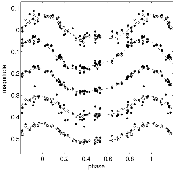
Figure 1: Smoothing of “observational” data (full dots) by the standard PCA method. Smoothed points are denoted by circles, dashed line represents the original unnoised light curves in five synthetic colours.

The application of PCA and WPCA should help us to find the number of parameters essential for the description of variability (number of mechanisms of variability in action), it enables us to examine relative quality of observations in multicolour measurements. Though we do not know $s_{j}$ of individual colours exactly, we could improve them very quickly using an iterative circle. The convergence of this process is pretty good, because the results are as a rule insensitive to the $s_{j}$ used.

Above mentioned methods help us namely in the preliminary processing of observational data, when we want to reach an orientation in the nature of variability of studied objects, possible relationships among measured quantities and their quality. All these information we can gain without using any physical model and time dependent smoothing, what can strongly embarrass finding a priori unexpected types of variability (rapid variations, trends etc.).

We demonstrate the PCA treatment of artificial photometric data (50 observations in 5 colours) simulating light variability of a rotating CP star with two differently coloured photometric spots. The “observed” points and smoothed points with suppressed noise for $r=2$ for individual colours are displayed in the phase diagram in the Fig. 1. The treatment have not taken into its consideration the phase information.

PCA methods similarly as LSM suffer from outliers which are quite common in astrophysical data. Introducing of weights in PCA enables us to eliminate their influence by means of an iterative process adjusting individual weights of entering data (see e.g. the appendix of [7]).

3 Advanced PCA

The extent of applicability of the standard and weighted PCA methods is rather limited as they are demanding to the completeness and homogeneity of input data. These confinements were obviously one of decisive reasons why the PCA techniques remain beyond the scope of the majority of observing astronomers.

Since 2000 we have developed a qualitatively new method synthesizing weighted PCA and robust regression. We will denote it as Advanced PCA (APCA). The versatility of APCA proves to be quite broad, it was used several times, see e.g. [4], [5], [6], however, it has not been fully described up to now. We will briefly present only the method, without its derivation and strict mathematical proving of lemmas or statements.

3.1 Vector description of light curves

Let the course of a light curve is described by means of preselected model the parameters of which are determined by standard regression methods, as LSM with weights or its modification eliminating the influence of outliers. It is advisable to use a linear model so that the course of a light curve in the certain colour $c$, $m_{c}(t)$ would be described by linear combination of the ensemble of $q$ so called elementary functions $f_{1}(t),f_{2}(t),\ldots f_{q}(t)$ defining the time dependence by the column vector of the length $q$: $\mathbf{f}(t)=[f_{1}(t);f_{2}(t);\ldots f_{q}(t)]$ by the relation:

$$\Delta m_{c}(t)=m_{c}(t)-\overline{m_{c}}=\sum_{i=1}^{q}\,y_{ci}\,f_{i}(t)=\mathbf{y}_{c}\,\mathbf{f}(t),$$ (7)

where $y_{ci}$ are components of a row vector $\mathbf{y}_{c}$, $\overline{m_{c}}$ is the mean magnitude in the colour $c$. The components of the vector are found from the observational data by standard regression procedures (weighted LSM, robust regression).

We should be very particular about the choice of the base of elementary functions $f_{1}(t),f_{2}(t),\ldots f_{q}(t)$. The functions should be selected so they enable us to express courses of all studied light curves of the object with sufficient accuracy. It is advisable for many reasons (avoiding of problems with multicollinearity, equality of the uncertainty of components of the vector $\mathbf{y}_{c}$) to opt elementary functions so that they would form the base quasiorthonormal on the set of data, what means:

$$\overline{f_{i}^{2}}\cong\overline{f_{j}^{2}}\cong\overline{f^{2}};\ \ \ \ \overline{f_{i}\,f_{j}}\ll\overline{f^{2}}\ \ \mathrm{for}\ i\neq j.$$ (8)

In the case the set of elementary functions does not obey above given conditions it is trivial to transform the system into orthonormal one by means of standard Gram-Schmidt’s orthonormalization procedure.

Assuming observational data be distributed more or less uniformly over the observational interval it is recommended to use Legendre polynomials orthonormal on the interval $\langle-1;1\rangle$. If the object is periodically variable then the condition of quasiorthogonality fulfill any combination of harmonic polynomials $\sin(2k\pi t/P),\ \cos(2k\pi t/P)$, $k=1,\,2,\ldots$; $\overline{f^{2}}=1/2$.

If the functions of the linear regression model are quasiorthonormal it is valid that uncertainties of particular components $\varepsilon_{c}$ of the vector $\mathbf{y}_{c}$ are the same:

$$\varepsilon_{c}\cong\frac{s_{c}}{\sqrt{N_{c}\,\overline{f^{2}}}};\ \ \ \ w_{c}\sim\varepsilon_{c}^{-2}\sim\frac{N_{c}}{s_{c}^{2}},$$ (9)

where $s_{c}$ is the standard deviation of the light curve fit, $N_{c}$ is the number of observations in the particular colour used for the light curve fit. The weight of the corresponding vector of light curve in the $c$-colour then will be proportional to the $\varepsilon_{c}^{-2}$.

The whole set of vectors describing the light curves in all $p$ colours can be arranged into the p$\times$q matrix $\mathbf{Y}$, with the weights described by the p$\times$p diagonal matrix $\mathbf{W}$.

3.2 Advanced PCA. Reducing free parameters. Usage of APCA

Let we permit that the variable part of light curves in all colours $\Delta m_{c}$ can be sufficiently accurately approximated by linear combination only $r$, ($r<q$) normalized orthogonal (principal) functions $\varphi_{j}(t)$ determined by linear combination of all $q$ elementary function $f_{i}(t)$ with coefficients forming the q$\times$r matrix $\mathbf{B}$:

$$\varphi_{j}(t)=\sum_{i=1}^{q}\,b_{ij}\,f_{i}(t)=\mathbf{b}_{j}\,\mathbf{f}(t).$$ (10)

$$\Delta m_{c}(t)=\sum_{j=1}^{r}\,k_{cj}\,\varphi_{j}(t)=\sum_{j=1}^{r}\,k_{cj}\mathbf{b}_{j}\,\mathbf{f}(t)=\mathbf{k_{\mathit{c}}\,{B\!}^{T}\,f}(t)=\mathbf{y_{s\!\mathit{c}}}\,\mathbf{f}(t),$$ (11)

$$\mathbf{y_{s\!\mathit{c}}}=\mathbf{k_{\mathit{c}}\,{B\!}^{T}},$$ (12)

where $\mathbf{b}_{j}$ is the normalized vector of the $j$-th principal function and $j$-th column of the matrix $\mathbf{B}$. The row vector $\mathbf{k}_{c}$ (1$\times$r) represents semiamplitude components of the light curve in colour $c$ versus $r$ principal functions $\{\varphi_{1}(t),\ldots\varphi_{r}(t)\}$ and the 1$\times$q vector $\mathbf{y_{s\!\mathit{c}}}$ contains parameters of the APCA smoothed light curve in the $c$ colour.

Further we will assume that the vector base $\{\mathbf{b}_{1},\ldots\mathbf{b}_{r}\}$ is orthonormal, then:

$$\mathbf{b}_{i}\,\mathbf{b}_{j}=\delta_{ij},\ \ \mathbf{{B\!}^{T}B=I}.$$ (13)

Minimizing the scalar quantity $S(\mathbf{B,k}_{c})$ defined as the the sum of weighted variances of differences $\Delta\mathbf{y}_{c}=\mathbf{y}_{c}-\mathbf{y_{s\!\mathit{c}}}$:

$$S(\mathbf{B,k}_{c})=\sum_{c=1}^{p}\Delta\mathbf{y}_{c}\,\Delta\mathbf{y}_{c}^{\mathbf{T}}\,w_{c}=\sum_{c=1}^{p}(\mathbf{y_{c}\,y_{c}^{T}-k_{c}\,k_{c}^{T}})\,w_{c};\ \ \ \mathrm{grad}S=\mathbf{0},$$ (14)

we arrive after some algebra at the following conclusions:

$$\mathbf{K=YB},\ \ \mathbf{(Y^{T}W\,Y)\,B=B\,(K^{T}W\,K)=B\Lambda}.\ \$$ (15)

$$\mathbf{Y_{s}=Y\,\widehat{B}=Y(B\,{B\!}^{T})}.$$ (16)

The results in equation (15) and (16) are formally identical with (4-6), so we can conclude that the matrix $\mathbf{B}$ contains $r$ column vectors which are eigenvectors of the matrix $\mathbf{Y^{T}W\,Y}$ corresponding to its first $r$ largest eigenvalues. The smoothing matrix $\mathbf{\widehat{B}}$ is defined identically, as $\mathbf{\widehat{A}}$.

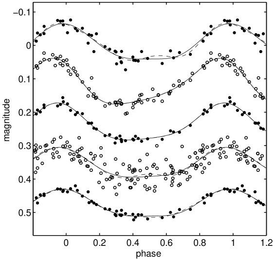
Figure 2: Fitting of “multicolour observational” data by advanced PCA method (full line). Dashed lines represent the fitting by the LSM.

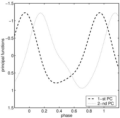
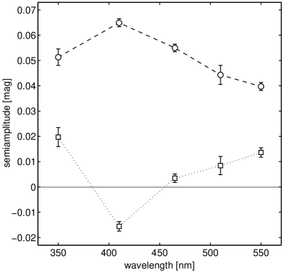
Figure 3: (a) The courses of first two principal functions. (b) The dependence of semiamplitudes on wavelength in nm for both principal components. Dashed lines – $1^{\mathrm{st}}$ principal component, dotted lines – $2^{\mathrm{nd}}$ principal component.

Nevertheless, we have to emphasize that the advanced PCA is not identical with standard PCA or WPCA. APCA and PCA give very similar but not the same results, smoothing matrix $\mathbf{\widehat{B}}$ is not the duplicate of $\mathbf{\widehat{A}}$! The main reason consists in the fact, that data treated by PCA have been centered to their mean, while in the case of APCA we handle directly with the found data without any centering. The difference is formulated in the basic suggestion of APCA (10), which seems to us physically more entitled than postulates of PCA. The correctness of APCA method has been verified using several relevant statistical tests and trials with simulated data.

We demonstrate the usage of APCA on synthetic photometric data simulating light variability of the same model of the rotating CP star. The Fig. 2 displays the phase diagram of multicolour light variations:“observed” points are marked by full dots, the light curves fitted by standard LSM technique are displayed by dashed lines. The light curves found by the APCA are plotted by full lines - they are indistinguishable from synthetic ones. The course of first two principal curves are displayed in the Fig. 3a, the dependencies of semiamplitudes versus both principal light curves are plotted in the Fig. 3b. From the course of diagram of real object we can gather on the nature of the light variability.

APCA can be used for reliable prediction of multicolour behaviour of the object, the method is very apt for the light curves quantification and classification [4], [6], for multicolour O-C measurements [5], for the light ephemeris improvement [4]. APCA seems to be a very efficient tool for the analysis of spectral variations and radial velocity measurements [3].

4 Conclusions

Principal Component Analysis and namely Advanced PCA proves to be an universal, relatively simple method with an extremely versatile extent of usage namely in the astronomical data (both photometric and spectroscopic) processing and interpretation. Efficiency and applicability of the PCA grows when we combine it with other sophisticated methods of the data treatment as e.g. robust regression, weighted LSM and wavelet analysis.

The author is very indebted for to Drs. Miloslav Zejda and Jan Janík for careful reading of the manuscript and valuable comments and suggestions. This investigation was supported by the Grant Agency of the Czech Republic, grants No. 205/04/2063 and No. 205/06/0217.

References

- [1] Jackson, J.E., A User’s Guide to Principal Components, Wiley, 2003
- [2] Jolliffe, I.T., Principal Component Analysis, 2nd ed., Springer, 2004
- [3] Korčáková, D., Mikulášek, Z., Kawka, A., Kubat, J., Hornoch, K. et al., 2005, IBVS 5605, 1
- [4] Mikulášek, Z., Gráf, T., 2005, Astrophys. Space Sci. 296, 157
- [5] Mikulášek, Z., Krtička, J., Zverko, J., Žižňovský, J., Janík, J., in the Proceedings of Active OB-Stars: Laboratories for Stellar Circumstellar Physics, S. Stefl, S. Owocki and A. Okazaki eds., ASP Conference Series Volumes, 2007, Vol. 361
- [6] Mikulášek, Z., Zverko, J., Žižňovský, J., Janík, J., in the Proceedings of The A-Star Puzzle, Poprad, Slovakia, J. Zverko, J. Žižňovský, S.J. Adelman, and W.W. Weiss eds., IAU Symposium, No. 224. Cambridge, UK: Cambridge University Press, 2004, 657
- [7] Mikulášek, Z., Žižňovský, J., Zverko, J., Polosukhina, N.S., 2003, Contr. Astron. Obs. Skalnaté Pleso 33, 29