An Improved Photometric Calibration of the Sloan Digital Sky Survey Imaging Data

Abstract

We present an algorithm to photometrically calibrate wide field optical imaging surveys, that simultaneously solves for the calibration parameters and relative stellar fluxes using overlapping observations. The algorithm decouples the problem of “relative” calibrations from that of “absolute” calibrations; the absolute calibration is reduced to determining a few numbers for the entire survey. We pay special attention to the spatial structure of the calibration errors, allowing one to isolate particular error modes in downstream analyses. Applying this to the Sloan Digital Sky Survey imaging data, we achieve $\sim 1\%$ relative calibration errors across 8500 deg² in $griz$; the errors are $\sim 2\%$ for the $u$ band. These errors are dominated by unmodelled atmospheric variations at Apache Point Observatory. These calibrations, dubbed “ubercalibration”, are now public with SDSS Data Release 6, and will be a part of subsequent SDSS data releases.

1. Introduction

A common challenge for all physics experiments is relating a detector signal to the underlying physical quantity of interest. Astronomical imaging surveys are no exception; a CCD camera counts Analog to Digital units (ADU) in each pixel, a quantity that is (approximately) proportional to the number of incident photons. This relationship must be calibrated to yield physical flux densities $(\rm{erg\,cm}^{-2}\rm{s}^{-1}\rm{Hz}^{-1})$. Key scientific programs of current and next generation imaging surveys demand ever more precise photometric calibrations. For example, wide field imaging surveys allow one to measure the clustering properties of galaxies (and therefore, the underlying dark matter) on scales otherwise accessible only in the Cosmic Microwave Background (CMB); comparing the CMB at redshift $z\sim 1000$ with the relatively recent Universe at $z\mbox{${}^{<}_{\sim}$}1$ allows increasingly precise tests of our cosmological model. The first such measurements of clustering on gigaparsec scales and larger were recently reported (Padmanabhan et al., 2007; Blake et al., 2007). These results emphasize the need for accurate photometric calibrations over wide areas; the underlying clustering signal is a rapidly decreasing function of scale, and could easily be overwhelmed by percent-level systematic errors in the photometric calibration. A second example is reconstructing the structure of the Galaxy, using the photometric properties of different stellar populations. There have been a number of efforts to do this with existing data (Juric et al., 2005), and it is a key scientific program for the next generation of imaging surveys. Finally, there is the general (and powerful) motivation that reducing systematic errors invariably reveals hitherto unseen details and avenues of enquiry. Leveraging the current and next generation of imaging surveys to yield their maximum scientific potential requires revisiting the problem of photometric calibration, moving beyond the simplifications currently made (Stubbs & Tonry, 2006). Several surveys are photometrically calibrated to a few percent; the challenge for the next generation of surveys is to deliver $<1\%$ calibrations over wide areas.

Photometric calibration involves relating the output of a CCD to the physical flux received above the Earth’s atmosphere. For wide-field imaging surveys, we separate this into two orthogonal problems - “relative” calibration, or the problem of establishing a consistent photometric calibration (albeit in possibly arbitrary flux units) across the entire survey region, and “absolute” calibration, which transforms the relative calibrations into physical fluxes. This separation is useful since there exist a number of applications (such as the two discussed above) that are relatively tolerant of errors in the absolute calibration, but demand precise relative calibrations. Current calibration techniques, which usually involve comparing observations to “calibrated standards”, do not respect this distinction, making it difficult to control errors in the relative calibration. Furthermore, calibrating off standard systems normally involve relating different telescope and filter systems, and are quickly limited by the accuracy with which these transformations can be measured. Accurate relative calibrations would therefore only use data from the native telescope/ filter system, obviating the need for any such transformations.

A second separation, emphasized by Stubbs & Tonry (2006) is to separate the “transfer function” of the telescope and detectors from that of the atmosphere. The telescope and detectors form an approximately closed system whose responses can be (potentially) mapped out with exquisite precision with laboratory equipment. The atmosphere, on the other hand, is an open, highly dynamical, system with a range of relevant time scales; the best one can do is to monitor it with limited precision. Although we agree with this separation in principle, applying it would go significantly beyond the scope of this paper. We therefore do not make this distinction in the analysis presented here, but we return to it at the end of this work.

Techniques for relative photometric calibration have been applied to optical imaging in the past, although much more limited than the present work in the scope of either the number of objects or the field of view. Landolt (1983) and Landolt (1992) are widely recognized as describing one of the best-established “photometric systems”. Landolt observed several hundred stars near the celestial equator with a photomultiplier tube on the Cerro Tololo 16-inch and the Cerro Tololo 1.5-m telescopes. Landolt achieved exceptional relative photometric calibrations in five broad optical bandpasses (Johnson-Kron-Cousins UBVRI). His data are accurate to 0.3% per observation of each star, with an even better accuracy implied for those stars that have many observations. Unfortunately, the full benefit of the accuracy of this photometric system cannot be realized for other surveys due to the systematic uncertainties in transforming from Landolt’s system responses to observations on other telescopes using (typically) CCD photometry. There are some observations using exactly the Landolt system, most famously of supernova 1987A, which made use of the otherwise-decommissioned Cerro Tololo 16-inch telescope (Blanco et al., 1987).

The other example of accurate relative optical photometry has come from the searches for massive compact halo objects (MACHOs) from microlensing events in dense star fields (e.g. Udalski et al., 1992; Alcock et al., 1993; Aubourg et al., 1993). MACHO events were detected from differencing images taken with an identical instrument over timescales of several years. More recently, these same techniques have been used to detect the optical transits of planets. With a proper treatment of the correlated noise properties in the time series of images (Pont et al., 2006), it is possible to detect transits with peak depths of only $\sim$1%. Note that the challenges here are different from the wide field imaging case considered in this work, since one is interested in differences in photometry of a single star.

Cosmic Microwave Background (CMB) anisotropy experiments also demand very precise relative calibrations. This accuracy is obtained with repeat observations of the sky, and cross-linked scan patterns. The redundancy thus obtained allows one to simultaneously solve for the CMB temperature at a given direction on the sky and the detector calibration parameters. In this paper, we propose adopting this technique as a new approach to calibrating optical imaging surveys - replacing the CMB temperature fluctuations with the magnitudes of stars. Note that as this involves comparing multiple observations, this is a differential measurement, and therefore only yields a relative calibration. However, while the absolute calibration still must be obtained by comparison against standard stars, this is now applied uniformly across the entire survey region. These ideas are not new to optical astronomy; precursors may be found in the work of Maddox et al. (1990); Honeycutt (1992); Fong et al. (1992); Manfroid (1993); Fong et al. (1994); Glazebrook et al. (1994). What is new to this work is both the (large angular) scales to which the method is applied and the accuracies obtained.

The Sloan Digital Sky Survey (York et al., 2000, SDSS) is one of the most ambitious optical imaging and spectroscopic surveys undertaken to date. It has imaged a quarter of the sky in five optical bands, and has spectroscopically followed up more than a million of the detected objects. This makes the SDSS both a scientifically rich data set and an excellent proving ground for the next generation of surveys. Accordingly, our goal in this paper is to develop the idea above in the context of the photometric calibration of the Sloan Digital Sky Survey (SDSS). We begin by recapitulating aspects of the SDSS essential to this algorithm in Sec. 2. Sec. 3 then presents the details of the algorithm. We then assess the performance of our calibrations with simulations of the SDSS; the results are in Sec. 4. We then present a recalibration of the entire SDSS imaging data in Sec. 5. Sec. 6 announces the release of this calibration to the public, and Sec. 7 concludes with a discussion of the features and limitations of this work, as well as its applicability to the next generation of imaging surveys. Although we focus on the SDSS, we phrase our discussion in terms that allow adapting the methods described here to arbitrary imaging surveys.

2. The SDSS

The Sloan Digital Sky Survey (York et al., 2000) is an ongoing effort to image approximately a quarter of the sky, and obtain spectra of approximately one million of the detected objects. The imaging is carried out by drift-scanning the sky in photometric conditions (Hogg et al., 2001), using a 2.5m telescope (Gunn et al., 2006) in five bands ($ugriz$) (Fukugita et al., 1996; Smith et al., 2002) using a specially designed wide-field camera (Gunn et al., 1998). These data are processed by completely automated pipelines that detect and measure photometric properties of objects, and astrometrically calibrate the data (Lupton et al., 2001; Pier et al., 2003). The first phase of the SDSS is complete and has produced seven major data releases (Stoughton et al., 2002; Abazajian et al., 2003, 2004, 2005; Adelman-McCarthy et al., 2006, 2007; Adelman-McCarthy & for the SDSS Collaboration, 2007).

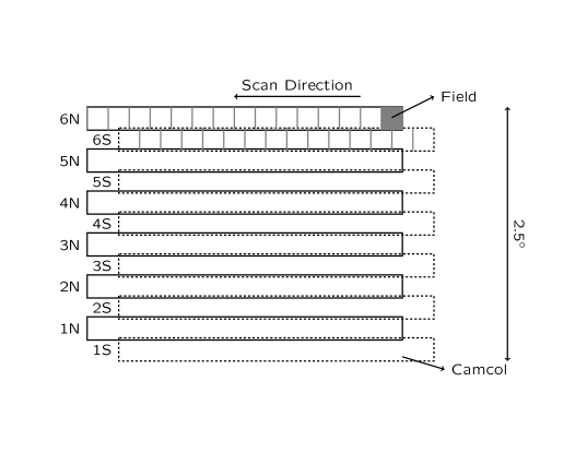
Figure 1.— The geometry of the SDSS imaging. Part of an SDSS stripe with the two interleaved strips (denoted by N and S) is shown. Each strip consists of six camcols (numbered 1 through 6 in the figure), while each camcol is further divided into fields (for simplicity, we show field divisions for only two camcols). See the text for more details.

The SDSS imaging data (see also Fig. 1) are taken by drift-scanning along stripes centered on great circles on the sky in all five filters. These stripes are $2.5^{\circ}$ wide, and are filled by two interleaved strips. The actual data is taken in runs, which are part of strips; multiple runs may be taken in a single night, not necessarily on the same strip. Each run is further subdivided into six camera columns or camcols, corresponding to the six columns of CCDs on the camera. The data from each CCD is in turn split into frames, consisting of 1361 drift scan rows. The five frames corresponding to the same region of sky observed in the five SDSS filters, are collectively referred to as a field. Note that while runs and camcols correspond to physical separations of the data, the division into frames is purely artificial. The integration time is approximately 54.1 seconds per frame in each filter, with a time lag of $\sim 73$ seconds between each adjacent filter. The order of the filters as they observe the sky is $riuzg$.

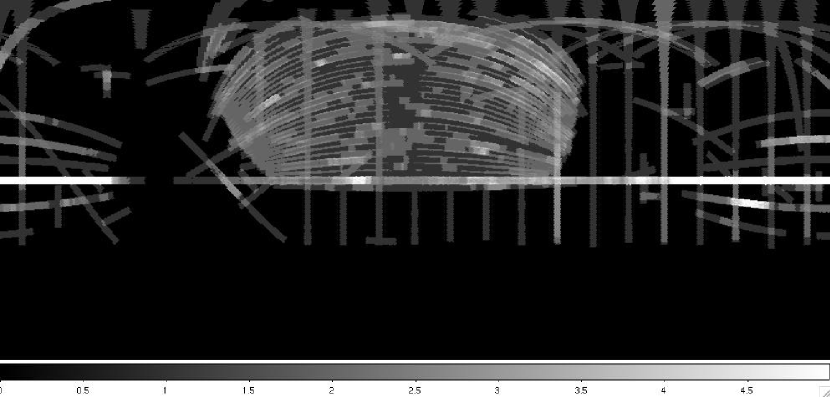
Figure 2.— The sky coverage of the SDSS data used in this paper, shown in an equal area resolution 7 HEALPIX/HEALCART (Górski et al., 1999; Finkbeiner, 2004) projection. The $x$ scale covers RA $0^{\circ}$ to $360^{\circ}$, while the $y$ axis runs from DEC $90^{\circ}$ to $-90^{\circ}$. The grey scale denotes the mean number of observations of a star in a particular pixel. Note that we saturate at 5 observations, although on the equatorial (white) stripe, there are pixels with a mean number of observations as high as 15. The bulk of the survey data is in the North Galactic Cap, the prominent structure in the center of the image. The Equatorial stripe, imaged every Fall, is the white horizontal stripe halfway in the image. The approximately equally spaced vertical runs are examples of the Apache Wheel data.

The current survey flux calibrations are applied in a three step process, involving three different telescopes and subtly different filter systems. The absolute flux system is defined by BD+17^∘4708 (Oke & Gunn, 1983), an F0 subdwarf star and is based on synthetic photometry in the expected (at the time) SDSS $u^{\prime}g^{\prime}r^{\prime}i^{\prime}z^{\prime}$ filters and an improved spectral energy distribution for this star (Fukugita et al., 1996). This is used to calibrate a primary network of 158 stars observed by the USNO 40-inch at Flagstaff in Arizona, chosen to span a range in color, airmass, and RA, and distributed over the Northern sky (Smith et al., 2002). Unfortunately, these stars saturate the SDSS survey telescope; the calibrations are therefore indirectly transferred via a 20 inch Photometric Telescope (PT) at Apache Point (APO), which observes these primary standards, as well as 1520 $41.5\times 41.5\,{\rm arcmin}^{2}$ secondary patches of sky. These patches are what finally calibrate the data from the 2.5m survey telescope (Tucker et al., 2006). Note that these are three different filter systems, and not just realizations of one system. In addition to conflating the absolute and relative calibrations, this indirect transfer of the calibration makes achieving $<1\%$ calibrations via this method a challenge, although it does return relative calibrations accurate to $\sim 2\%$ (Ivezić et al., 2004). Note that these errors have natural scales of $2.5^{\circ}/12$ (the width of a camcol) and $2.5^{\circ}$ (the width of a stripe) perpendicular to the scan direction.

Before continuing, it is worth emphasizing that $2\%$ calibrations for a wide field optical survey was unprecedented until very recently. However, motivated by the promise of future wide field surveys and the challenge of $1\%$ photometry, we realized that the next step must short-circuit the above multi-stage calibration pipeline. The calibration algorithm we propose here relies on repeat observations to constrain the photometric calibrations. Unfortunately, in the standard survey strategy, the only significant repeat observations occur at the poles of the survey (where the great circles of stripes converge), and on the celestial equator, which is re-imaged every Fall (see Fig. 2). While the Fall equatorial stripe has sufficient repeat observations to make precise photometry possible (Ivezić et al., 2007), the calibration for the bulk of the survey region would only be constrained at the survey poles, clearly undesirable. The only other natural overlaps occur when the beginning and ends of runs overlap each other along strips. While this does connect the survey from one pole to the other, most of the overlaps occur on the same CCD column, and so have limited utility since these are degenerate with flat fields.

To address both these inadequacies, two additional sets of data were taken. The first were short scans that cross the normal scan directions. Such oblique scans exist for most observing years (Fall through Spring), and were taken to check for temporal variations of the flat fields. These are invaluable for constraining flat fields, since they compare each CCD column with every other. The other data were a grid of long scans, dubbed the “Apache Wheel”, designed to connect every part of the survey with every other. Observing such a grid with the usual SDSS scanning speed would have required a significant expenditure of telescope time, adversely affecting the science goals of the survey. The compromise was to observe these data, at 7 times the normal scanning speed (i.e. with an effective exposure time of $\sim 8$ seconds), and binning data into 4x4 native camera pixels. Reducing these data required modifications to the survey data reduction pipelines (Lupton et al., 2001), and was done at Princeton (along with a re-reduction of regular survey data) as part of this calibration effort. The survey region we consider in this paper is in Fig. 2, with the greyscale encoding the number of repeat observations of different regions of the sky.

3. The Algorithm

3.1. The Photometric Model

An introduction to photometric calibrations and photometric standard systems may be found in Bessell (2005); we focus on the details relevant to this work below. Assuming linearity, the flux $f$ of an object at Earth (above the atmosphere) is related to the detected flux $f_{ADU}$ by

$$f={\cal K}f_{ADU}\,\,;$$ (1)

the problem of photometric calibration is to determine ${\cal K}$. The above equation is deceptively compact; ${\cal K}$ depends on the exposure time, detector efficiency, filter responses, the telescope optical system, the optical path through the atmosphere, the spectral energy distribution of the objects in question, and all the variables that these in turn are sensitive to. Furthermore, Eq. 1 makes no reference to the units of $f$ and ${\cal K}$; the problem of determining the correct units is that of absolute photometric calibration; we restrict our discussion below to the problem of relative calibrations.

Since all the above terms affect the flux multiplicatively, it is convenient to work in log-space; the above effects become additive corrections. Converting fluxes to magnitudes ($m=-2.5\log_{10}f$), Eq. 1 becomes

$$m=m_{ADU}-2.5\log_{10}({\cal K})\,\,.$$ (2)

Expanding ${\cal K}$ in terms of its various dependencies, we obtain

$$-2.5\log_{10}({\cal K})=a(t)-k(t)x+f(i,j;t)+...\,\,,$$ (3)

where all terms are a function of time. The optical response of the telescope and detectors is the “a-term” $a(t)$, while the detector flat fields (in magnitudes) are $f(i,j;t)$ where $i,j$ represent CCD coordinates. The atmospheric extinction is the product of the “k-term” $k(t)$ and the airmass of the observation, $x$. Note that this is a crude phenomenological model (it heuristically resembles a first order Taylor expansion), but is completely adequate for our purposes. We therefore defer a discussion of its limitations and potential extensions to Sec. 7.

Table 1 Flat Field seasons

SDSS Run	MJD	Date	Comments
1	51075	19-Sep-1998	Beginning of Survey
205	51115	28-Oct-1998
725	51251	13-Mar-1999
941	51433	12-Sep-1999
1231	51606	03-Mar-2000
1659	51790	03-Sep-2000	After i2 gain change
1869	51865	17-Nov-2000	Vacuum leak in Dec 2000
2121	51960	20-Feb-2001	After vacuum fixed
2166	51980	12-Mar-2001
2504	52144	23-Aug-2001	After summer shutdown
3311	52516	30-Aug-2002	After summer shutdown
4069	52872	20-Aug-2003	After summer shutdown
4792	53243	26-Aug-2004	After summer shutdown
5528	53609	26-Aug-2005	After summer shutdown

We now specialize to the SDSS; we calibrate each of the five filters individually, and assume that each of the six camera columns are independent, yielding an a-term and flat field to be determined per CCD. We implicitly assume that the filter response for each of the six CCDs is identical (we return to this in Sec. 7). The k-term is however common to all camera columns and depends only on the filter. Also, since the SDSS observes by drift-scanning the sky, the flat fields are no longer two-dimensional, but only depend on the CCD column and are represented by a 2048 element vector. This is complicated by the fact that some of the SDSS CCDs have two amplifiers, resulting in a discontinuity at the center of the flat field. We model this by assuming the flat fields have the form,

$$f(i,j)=f_{0}(j)+\theta(j-1024)\Delta f$$ (4)

where $\theta(x)$ is the Heaviside function, and $\Delta f$ (hereafter, the “amp-jump”) is the relative gain of the two amplifiers. Note that as written, $f_{0}$ is a continuous function of CCD column. Finally, we need to specify the time dependence of these quantities. The a-terms and amp-jumps are assumed to be constant during a night, and we simply specify these as piecewise constant functions.

It was also realized early in the survey (about 2001) that the flat fields were time-dependent, and appeared to be changing discontinuously over the summers when the camera was disassembled for maintenance. These changes are most likely associated with changes in the surface chemistry of the CCDs. We therefore model the flat fields as being constant in time over a “flat field season”, roughly the period between any maintenance of the camera. The boundaries, in MJD and SDSS run number, of these “seasons” are listed in Table 1. Ideally, one might have chosen an even finer time interval to test the constancy of the flat fields; however, the SDSS lacks sufficient oblique scan data to improve the time resolution. We note here that the standard practice of measuring flat fields from sky data does not work for the SDSS, due to scattered light in the camera.

The time dependence of the k-terms at APO is more complicated, as the atmosphere (on average) gets more transparent as the night progresses, at the rate of $\sim 1$ mmag/hour (millimagnitudes/hour) per unit airmass. We therefore model $k(t)$ over the course of a night as

$$k(t)=k+\frac{dk}{dt}(t-t_{ref})\,\,,$$ (5)

where $t_{ref}$ is a reference time. Note that $t$ in the above equation only runs over the course of a single night; $k$ and $dk/dt$ can (in principle) vary from night to night, and there is no requirement on the continuity of $k(t)$ across nights. Table 2 summarizes the parameters in our photometric model, whose final form is

$$m=m_{ADU}+a_{\alpha}-\left[k_{\beta}+\left(\frac{dk}{dt}\right)_{\beta}(t-t_{\beta,ref})\right]x+f_{\gamma}(j)\,,$$ (6)

with $\alpha$, $\beta$, and $\gamma$ indexing the appropriate a-term, k-term (and $t_{ref}$), and flat field for the star in question.

Table 2 Calibration Parameters

Parameter	Number	Fit	Comments
a-terms	$6\times 5\times n_{night}$	Yes
$k$	$5\times n_{night}$	Yes	k-term at $t=t_{ref}$
$dk/dt$	$5$	No
Flatfields	$6\times 5\times n_{season}$	Yes	2048 element vector
		(iterative)
Ampjumps	$6\times 5\times n_{run}$	No

3.2. Solution

Having specified the parameters of the photometric model, we now turn to the problem of determining them. It is natural to consider repeat observations of stars to constrain these parameters. Let us therefore consider $n_{obs}$ observations with observed instrumental magnitudes $m_{ADU,j}$, of $n_{star}$ unique stars with unknown true magnitudes $m_{i}$. Note that $n_{obs}$ is the number of observations of all stars, i.e. $n_{obs}=\sum_{i=1}^{n_{star}}n_{i}$ where $n_{i}$ is the number of times star $i$ is observed. Using Eq. 6, we construct a $\chi^{2}$ likelihood function for the unknown magnitudes and photometric parameters,

$$\chi^{2}[a_{\alpha},k_{\beta},(dk/dt)_{\beta},f_{\gamma}]=\sum_{i}^{n_{star}}\chi^{2}_{i}\,\,,$$ (7)

with

$$\chi^{2}_{i}=\sum_{j\in{\cal O}(i)}\left[\frac{m_{i}-m_{j,ADU}-a_{\alpha(j)}+k_{\beta(j)}(t)x-f_{\gamma(j)}}{\sigma_{j}}\right]^{2}\,,$$ (8)

where $j$ runs over the multiple observations, ${\cal O}(i)$, of the $i^{th}$ star, $\sigma$ is the error in $m_{j,ADU}$, and $k(t)$ is given by Eq. 5. We also assume that errors in observations are independent; this is not strictly true as atmospheric fluctuations temporally correlate different observations. One can generalize the above to take these correlations into account and, as we show below, our results are not biased by this assumption. Note that Eq. 7 has $n_{obs}$ known quantities, and $n_{star}+\#({\rm parameters})$ unknowns. In general, the number of photometric parameters $\ll n_{star}$, and $n_{obs}>2n_{star}$, implying that this is an overdetermined system.

To proceed, we start by minimizing Eq. 7 with respect to $m_{i}$; this yields,

$$\frac{d\chi^{2}}{dm_{i}} =2\sum_{j\in{\cal O}(i)}\left[\frac{m_{i}-m_{j,ADU}-a_{\alpha(j)}+k_{\beta(j)}(t)x-f_{\gamma(j)}}{\sigma_{j}^{2}}\right]$$ (9)

$$=0\,,$$

which is trivially solved for $m_{i}$ to give,

$$m_{i}=\sum_{j\in{\cal O}(i)}\left[\frac{m_{j,ADU}+a_{\alpha(j)}-k_{\beta(j)}(t)x+f_{\gamma(j)}}{\sigma_{j}^{2}}\right]$$

$$\times\left[\sum_{j\in{\cal O}(i)}\left(\frac{1}{\sigma_{j}^{2}}\right)\right]^{-1}\,.$$ (10)

As substituting the above result into Eq. 9 to solve for the calibration parameters is algebraically unwieldy, we reorganize these results by making the following notational change. We arrange the unknown photometric parameters into an $n_{par}$ element vector ${\bf p}$,

$${\bf p}=\left(\begin{tabular}[]{c}$a_{\alpha}$\\ $k_{\beta}$\\ $(dk/dt)_{\beta}$\\ $f_{\gamma}$\\ \end{tabular}\right)\,\,.$$ (11)

Then substituting Eq. 3.2 into Eq. 8 yields a matrix equation for $\chi^{2}$,

$$\chi^{2}=({\bf Ap-b})^{t}{\bf C}^{-1}({\bf Ap-b})\,\,,$$ (12)

where ${\bf A}$ is an $n_{obs}\times n_{par}$ matrix , and ${\bf b}$ is an $n_{obs}$ element vector, and ${\bf v}^{t}$ represents the transpose of ${\bf v}$. The errors are in the covariance matrix ${\bf C}$ which, in Eq. 8, is assumed to be diagonal (but can be generalized to include correlations between different observations). For clarity, we explicitly write out the form of ${\bf Ap-b}$ for the case of a single star observed twice at airmass $x_{1}$ and $x_{2}$, and with errors $\sigma_{1}$ and $\sigma_{2}$, where only the a- and k-terms are unknown,

010−x2)−(I1I2−x1I1−x2I2I1I2−x1I1−x2I2)]delimited-[]fragments 010fragmentsx2fragmentsI1fragmentsI2fragmentsx1I1fragmentsx2I2fragmentsI1fragmentsI2fragmentsx1I1fragmentsx2I2\displaystyle\left[\left(\begin{tabular}[]{cccc}1&0&$-x_{1}$&0\\ 0&1&0&$-x_{2}$\\ \end{tabular}\right)-\left(\begin{tabular}[]{cccc}$I_{1}$&$I_{2}$&$-x_{1}I_{1}$&$-x_{2}I_{2}$\\ $I_{1}$&$I_{2}$&$-x_{1}I_{1}$&$-x_{2}I_{2}$\\ \end{tabular}\right)\right]

10-x1010-x10 (17)

$$\times\left(\begin{tabular}[]{c}$a_{1}$\\ $a_{2}$\\ $k_{1}$\\ $k_{2}$\\ \end{tabular}\right)$$ (22)

$$-\left(\begin{tabular}[]{c}$m_{1,ADU}-m_{1,ADU}I_{1}-m_{2,ADU}I_{2}$\\ $m_{2,ADU}-m_{1,ADU}I_{1}-m_{2,ADU}I_{2}$\\ \end{tabular}\right)\,\,,$$ (25)

where $I_{i}$ is the normalized inverse variance, $I_{i}=\sigma_{i}^{-2}/\sum_{j}\sigma_{j}^{-2}$. Each row of ${\bf Ap-b}$ has a simple interpretation as the difference between the magnitude of a particular observation of a star, and the inverse variance weighted mean magnitude of all observations of that star. Also, although ${\bf A}$ is a large matrix ($\sim 50,000,000\times 2000$ for the SDSS), it is extremely sparse, and amenable to sparse matrix techniques.

Obtaining the best fit photometric parameters simply involves minimizing Eq. 12. Although there are several choices here, we proceed via the normal equations (e.g., Press et al., 1992),

$$\frac{d\chi^{2}}{d{\bf p}}={\bf A}^{t}{\bf C}^{-1}{\bf Ap}-{\bf A}^{t}{\bf C}^{-1}{\bf b}=0\,\,.$$ (26)

The inverse curvature matrix,

$$\frac{d^{2}\chi^{2}}{dp_{i}dp_{j}}=\left({\bf A}^{t}{\bf C}^{-1}{\bf A}\right)_{ij}\,\,,$$ (27)

provides an estimate of the uncertainty in the recovered parameters. Note that it is however not the covariance matrix of the parameters, since Eq. 12 was derived marginalizing over the unknown magnitudes of all the stars. Furthermore, since the measurement errors do not account for temporal variations in the atmosphere, the “error” estimates from the curvature matrix may be significantly underestimated.

We conclude by noting the similarities between the above and algorithms used for making maps of the CMB (e.g. Tegmark, 1997) . The SDSS runs are analogous to CMB scan patterns, while the magnitudes are equivalent to the temperature measurements. However, unlike the CMB, our principal goal is the calibration parameters, with the magnitudes of the stars being a secondary product.

3.3. Degeneracies and Priors

Our choice of photometric parameters is non-minimal in that there exist degeneracies between them. These degeneracies are of more than academic interest, as they make the normal equations singular, and solutions of them unstable. We now discuss the source of these degeneracies, and how the resulting numerical instabilities can be tamed by the use of priors.

• Zero point : As the above algorithm is based solely on magnitude differences, any overall additive shift of all the a-terms does not change $\chi^{2}$. Note that this is simply the problem of absolute calibration rephrased.

• Disconnected Regions : This is a generalization of the previous case; the zero points of each disconnected region of the survey can be individually changed, without changing $\chi^{2}$. Note that disconnected in this context refers regions with neither spatial nor temporal overlap (as we assume the photometric parameters are stable over the course of a night) with other parts of the survey.

• Zero point of flats : In Eq. 6, the zero point of the flat fields is degenerate with the a-terms; this degeneracy is trivially lifted by forcing the flat fields to have zero mean.

• Constant Airmass : The photometric equation schematically is $\sim a-kx$; therefore for data with little or no airmass variation, there is a degeneracy direction that keeps $a-kx$ constant, while changing both the a- and k-terms. While this does not affect the calibration in regions where $a-kx$ is constrained, extrapolating the a- and k-terms to regions with different airmasses can result in incorrect calibrations.

There is a useful generalization of the above discussion; the inverse eigenvalues of the curvature matrix (Eq. 26 and 27) are a measure of the error on the determination of linear combinations of the photometric parameters (encoded by the corresponding eigenvectors). The degeneracies discussed above are characterized by eigenvalues $\sim 0$, which make the normal equations unstable. However, any badly constrained combinations (even if they are formally well determined) can amplify noise and un-modeled systematics in the data, potentially introducing errors when the calibrations are applied. We therefore identify all eigenvectors of photometric parameters that are poorly constrained (i.e. those that could result in potential errors of $>$ 1% ), and project these out; this renders the normal equations stable and they can be directly solved. Note that this introduces a tunable parameter to the solution - the eigenvalue threshold below which we project out modes. This threshold is chosen such that the final calibrations are insensitive to its exact value.

Although projecting out poorly determined eigenvectors yields a minimal set of parameters well constrained by the data, we must add back in these “null” eigenvectors to get a solution in our original (and preferred) parameter space. We achieve this by introducing priors on the photometric parameters, and then adjusting the values of all the photometric parameters along the null vectors to best satisfy these priors. Assuming equally weighted Gaussian priors on the parameters ${\bf p}$ with a mean value ${\bf p}_{0}$, this can be phrased as an auxiliary $\chi^{2}$ minimization,

$$\chi^{2}_{\rm prior}=|{\bf\hat{p}^{\prime}}+{\bf V}_{null}\delta{\bf x}-{\bf p}_{0}|^{2}\,\,,$$ (28)

where ${\bf\hat{p}^{\prime}}$ is the solution of the normal equations, Eq. 26, and we have gathered the $n_{degen}$ null eigenvectors into a $n_{par}\times n_{degen}$ matrix ${\bf V}_{null}$. Varying $\delta{\bf x}$ to minimize $\chi^{2}_{\rm prior}$, we obtain our final solution for the photometric parameters,

$${\bf\hat{p}}={\bf\hat{p}^{\prime}}+{\bf V}_{null}\delta{\bf x}\,\,.$$ (29)

3.4. Implementation Details

The above discussion described our calibration algorithm in generic terms, with minimal reference to survey specifics. We now discuss the details and approximations specific to implementing this algorithm for the SDSS.

The first approximation involves determining the flat field vectors. As described, the flat field vectors are determined simultaneously with the other photometric parameters. Doing so would however have approximately doubled the number of photometric parameters, and significantly complicated the degeneracies between the various parameters. We therefore chose an iterative scheme where the flat fields are held constant while the other parameters are determined. We then use the best fit solution to measure the magnitude differences between multiple observations as a function of CCD column, and fit a flat field vector to these via a quadratic B-spline with 17 uniformly spaced knots. As we show in the next section, this scheme rapidly converges to the true solution. In addition, the SDSS photometric pipeline estimates the amp-jumps by requiring that the background be continuous across the amplifiers. Instead of fitting to the amp-jumps, we simply hold them fixed to these values.

The second approximation involves the k-terms and their time derivatives. The typical airmass variations over the course of a single night tend to be small, making the determination of k-terms very degenerate with the a-terms, as discussed in the previous section. The situation is even more degenerate for the time derivative of the k-terms. We fix these degeneracies by using priors for the k-terms, and fixing their time derivatives to values estimated by the SDSS photometric telescope (Hogg et al., 2001). Table 2 summarizes which parameters are fit in our implementation, while Table 3 lists the mean values for $k$ and $dk/dt$.

We must also specify the actual objects used for calibrating. We restrict ourselves to objects that the SDSS classifies as stars, and use aperture (7.43 arcsecond radius) photometry to determine their magnitudes. The first choice sidesteps the subtleties of galaxy photometry, while aperture photometry avoids aliasing errors from the point spread function (PSF) estimation into the calibration. The magnitude limits we use are in Table 3, along with the number of unique stars, and observations. We choose not to make any color cuts on the stars to eliminate variable stars and quasars. These only add noise to any calibrations, but cannot bias the results; we therefore just use outlier rejection ($3\sigma$ clipping) and iterate our algorithm to minimize such contamination. A significant advantage of this approach is that the calibration of the 5 SDSS filters is independent, allowing us to use colors of sub-populations of stars as external tests of the calibrations; this is discussed in detail in Sec. 5.4.

Our algorithm does assume that the input data were taken under photometric conditions. We therefore, at the outset, eliminate all data taken under manifestly non-photometric conditions. As we discuss below, the algorithm does provide diagnostics of the photometricity of the data; we therefore iterate the algorithm removing any remaining non-photometric data.

Table 3

Filter	Mag.	$n_{star}$	$n_{obs}$	$k_{0}$	$dk/dt$	$\sigma(dk/dt)$
	Limit	$(\times 10^{6})$	$(\times 10^{6})$		$(\times 10^{2})$	$(\times 10^{2})$
$u$	18.5	4.7	14.6	0.49	- 1.2	2.5
$g$	18.5	9.3	29.1	0.17	-0.7	1.7
$r$	18.0	11.7	36.5	0.10	-1.0	1.7
$i$	17.5	11.5	35.9	0.06	-1.2	1.5
$z$	17.0	11.6	36.4	0.06	-2.2	1.7

Finally, there remains the issue of the absolute calibration of these data, or determining the five zero points for each filter. Improving the absolute calibration is beyond the scope of this paper; we therefore determine the zero points by matching magnitudes on average to those obtained by the standard SDSS calibration pipeline. These are therefore essentially on an AB system (Abazajian et al., 2004), tied to the SDSS fundamental standard, BD+17^∘4708 (Oke & Gunn, 1983).

4. Simulations

Simulations serve the dual purpose of verifying the above algorithm and our implementation of it, as well as quantifying the level of residual systematics. We construct the simulations as follows :

• We start with the actual catalog of stars observed by the SDSS, with the magnitude cuts described above. This ensures (by construction) that the pattern of overlaps in the simulations matches the observed data, essential to obtaining realistic results.

• We simulate “true” magnitudes for each of the stars, using a power law distribution, where the normalization and slope are matched to their observed values.

• Given an observation of the star, we then transform the magnitude into an observed instrumental magnitude, assuming values for the a- and k-terms and flat fields. We simulate the time variation of the k-term by describing $k(t)-k_{0}$ by a Gaussian random walk in time, with a drift in time given by $dk/dt$. The size of the steps is set by the observed value of the scatter in $dk/dt$ (Table 3). Note that this random component attempts to model the correlations in time induced by the atmosphere, albeit by making the simplification that the spectrum of fluctuations is described by a Gaussian random walk. Non-photometric data is simulated by exactly the same process, although we arbitrarily increase the scatter in the random walk.

• We add noise to the instrumental magnitudes by considering the Poisson noise from both the object and the sky. Note that the Poisson fluctuations from the sky dominate the error budget for most of the objects.

These simulated catalogs are structurally identical to the actual data. We can therefore analyze them in exactly the same manner, and compare the derived parameters with those input, providing us with an end-to-end test of our pipeline. Furthermore, these simulations have exactly the same footprints, timestamps and overlap patterns as the real data, allowing us to estimate our final errors and explore parameter degeneracies.

4.1. Results

Figs. 3 and 4 show the differences between the true and estimated a- and k-terms, and flat field vectors for the $r$ band in one of our simulations, analyzed identically to the real SDSS data. The flat field vectors are recovered with an error $<0.5\%$. The SDSS pipeline stores flat fields as scaled integer arrays; the roundoff error from this is about an order of magnitude lower. The a- and k-terms are similarly correctly estimated on average, although there are significant misestimates for both. However, a striking feature of Fig. 3 is the similarity in the residuals for the a- and k-terms, reminiscent of the discussion of the degeneracies between the a- and k-terms in Sec. 3.3. This suggests comparing the estimated and true values of $a-k\langle x\rangle$ on a per-field basis, where $\langle x\rangle$ is the average airmass over a given field and filter; it is this combination that determines the photometric calibration of a field.

Table 4 Calibration Errors

Filter	$\langle\Delta m\rangle$	$\sigma$	$\sigma_{3}$	$\%(3\sigma)$	$\sigma_{0}$
$u$	-1.67	13.38	12.53	0.85	7.25
$g$	0.82	7.79	7.31	0.72	1.77
$r$	0.93	7.81	7.26	0.81	1.69
$i$	0.92	6.84	6.38	0.75	1.32
$z$	0.97	8.06	7.61	0.68	2.70

The results of this comparison are in Table 4.1. We start by noting that the calibrations are determined correctly (on average) to $\sim 0.1\%$ or better, verifying both the algorithm and our implementation of it. The errors in the calibrations are $<1\%$, or $10$ mmags for all the filters (except $u$, where they are slightly higher), suggesting that the SDSS can break the “sound barrier” of delivering $1\%$ relative calibrations over the entire survey region. Catastrophic failures in the calibrations are also negligible, evidenced both from the near equality between the sigma-clipped and total variances, and the almost Gaussian fraction of $3\sigma$ outliers. Finally, we note that the errors in the calibrations are dominated by the unmodeled random fluctuations in the k-terms. Simulations with no random fluctuations achieve calibration errors of $\sim 0.1\%$, suggesting that the SDSS calibration errors are therefore completely dominated by unmodeled behaviour in the k-terms. The exception again is the $u$ band where measurement noise is only a factor of $\sim 2$ smaller than the random noise in the atmosphere.

Figure 3.— The difference between the estimated and true a- and k-term for the $r$ band in one of our simulations. There are approximately 6 a-terms that correspond to a given k-term, and the scales on the $x$ axis are adjusted so that corresponding terms are aligned. Note that the estimated a- and k-terms are highly covariant.

The spatial distribution of the calibration errors is in Fig. 5. The calibrations are uniform across the whole survey area at the $\sim 1\%$ level, and are noticeably better at the survey poles where the number of overlap regions increases (see Fig. 2). Importantly, although there is spatial structure over individual SDSS runs (which is inevitable, given that we calibrate entire runs as atomic units), there are no coherent structures over the entire survey region.

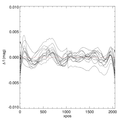
Figure 4.— The difference between the estimated and true flat field vectors for the $r$ band of one of our simulations. Each line corresponds to a different flat field season. Since the mean of the flat fields are degenerate with the a-terms, we only plot the deviations about the mean. For clarity, only the flat field vectors for one camera column are plotted; the results for the other camera columns are similar. The errors in the flat field estimation are $\sim 0.5\%$ (peak to peak).

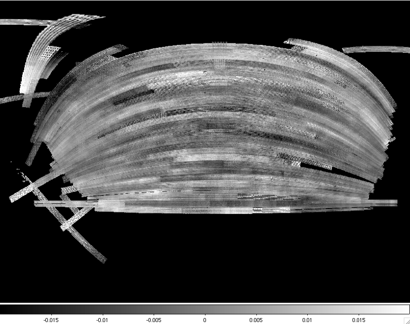
Figure 5.— An image of the calibration errors for $r$ band on the sky obtained for one of our simulations. The projection is the same as Fig. 2, but zoomed in on the Northern Galactic Cap of the SDSS. The greyscale saturates at magnitude errors of $\pm 0.02$ mag.

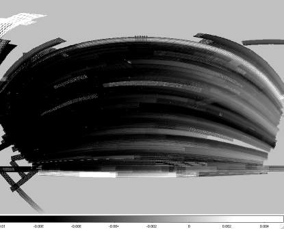
Figure 6.— The difference in calibration between assuming $dk/dt=0$ and the true value. The tilt over the survey region is clearly apparent, and is approximately 10 mmag over the survey region. The greyscale goes from $-0.01$ mag to $+0.005$ mag.

The above discussion assumes calibrations making the default choices described in Sec. 3.4. We can use our simulations to discuss the robustness of the algorithm to these choices below. For simplicity, we only consider the $r$ band for these tests.

• Magnitude Limits : As discussed above, the errors in the calibration are dominated by unmodeled systematics in the atmosphere, and not measurement noise. We therefore expect the algorithm to be relatively insensitive to the choice of the magnitude limit. We explicitly verify this by re-calibrating after decreasing the magnitude limit by 0.5 mag. Although this reduces the number of stars and observations by 30%, the calibration errors are unaffected, as expected.

• Apache Wheel data : As described in Sec. 2, the SDSS imaging data was supplemented by a grid of 4x4 binned data designed to improve the uniformity of the calibration over the entire survey region. Calibrating the survey without these data increases the calibration error to 10.4 mmag (compared with the 7.8 mmag in Table 4.1), an increase of $\sim 30\%$. Most of this increase is however driven by catastrophic failures; the $3\sigma$ clipped variance only increases to 8.1 mmag, a more modest increase of 10%. As expected, the Apache Wheel data better constrain parts of the survey that were poorly connected, as they were designed to do. However, for regions already well constrained, the improvements are marginal.

• $dk/dt$ : Since we do not fit for a value of $dk/dt$, we must understand how errors in our assumed value of $dk/dt$ propagate to the calibration. Fig. 6 shows the difference between calibrating a simulation assuming the correct value of $dk/dt$, and assuming $dk/dt=0$. While the increase in the size of the calibration errors is small, the incorrect value of $dk/dt$ introduces an overall tilt to the survey (in the figure, this is approximately 10 mmag). This tilt results from the fact that regions of similar RA are observed at approximately the same relative time in the night. The errors from an incorrect $dk/dt$ therefore do not cancel, but accumulate into a tilt, because we always observe the sky west to east. This is exacerbated by the fact that there is little data connecting the survey at the ends through the Galactic plane, and therefore no closed loops to prevent the appearance of such a tilt. This is the most serious systematic error in the calibration, and could affect any large scale statistical measures. In fact, both Padmanabhan et al. (2007) and Blake et al. (2007) observe excess clustering of photometrically selected luminous red galaxies at the very largest scales. We speculate that a tilt in the calibration could be a possible contaminant to the measurements on those scales.

5. The SDSS Photometric Calibration

Having described and verified our algorithm, we apply it to the SDSS imaging data. Since we do not have ground truth to compare our results, we describe both the internal consistency (Sec. 5.1) and astrophysical tests (Sec. 5.4) we use to assess the photometric calibration. In addition, we also address the spatial structure of the calibration errors (Sec. 5.2), as well as the photometric stability of the SDSS (Sec. 5.3). Finally, we compare our calibrations with the currently public SDSS calibrations (Sec. 5.5).

In what follows, we use “magnitude residual” to denote the difference between the (calibrated) magnitude of an observation of a star and the mean magnitude of all observations of the star.

5.1. Internal Consistency

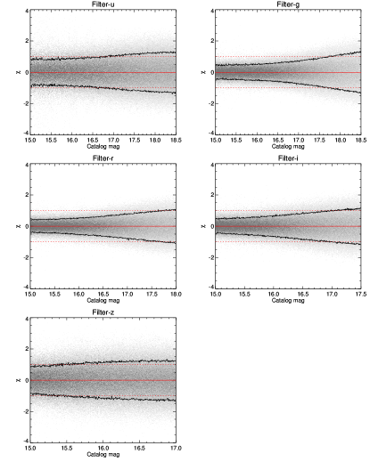
Figure 7.— The magnitude residuals weighted by their errors ($\chi$) as a function of apparent magnitude, for the five SDSS filters. The residual for a given observation is the difference between the observed magnitude and the mean magnitude averaged over all the observations of the star. The dotted lines show $\chi=\pm 1$, while the solid lines show the 16% and 84% contours; these should coincide with the $\chi=\pm 1$ lines if the scatter in the magnitudes is well described by the errors. The discrepancy at bright magnitudes is due to an error floor we impose to down-weight the brightest stars.

The first internal consistency test is the distribution of magnitude residuals. Since the scatter in the residuals also includes measurement noise ($\sigma$), it is more illuminating to consider $\chi=(m-\langle m\rangle)/\sigma$; if the measurement errors are a good estimate of the scatter in the residuals, $\chi$ should be Gaussian distributed with unit standard deviation. This is plotted for the stars used in the calibration, for the five filters, in Fig. 7. At the faint end, we observe that $\chi$ is distributed as expected, suggesting that the measurement noise is a good description of the scatter, and that calibration errors do not appreciably increase the scatter. The discrepancy at the bright end is due to a floor ($\sigma=0.01{\rm mag}$ added in quadrature) we impose on the magnitude residuals, to reflect the fact that the dominant error for these stars is no longer Poisson noise but possible systematics in the measurements. Note that calibration errors would only broaden the distribution of $\chi$.

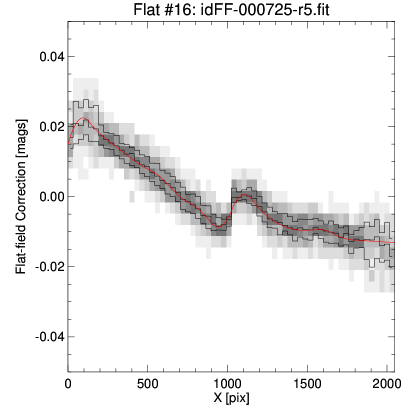
Figure 8.— An example of a flatfield vector from one $r-$band chip during Season 3. The grey scale and 25%, 50%, and 75% contours show the magnitude residuals as a function of CCD column, for all stars observed multiple times during that season. The smooth central (red) line shows the best fit (splined) flatfield vector.

We also consider the magnitude residuals as a function of the CCD column, grouping the data by CCD and flat field seasons; this is an estimate of the accuracy of our flat field correction. An example of these magnitude residuals as a function of the CCD column for camcol 5 in $r-$band is shown in Fig. 8. We don’t correct for the flat field in this plot, to show the structure of the flat field itself. The r.m.s scatter in the magnitude residuals about the derived vector is $\sim 0.5$% throughout the chip, although it increases at the edges of the CCD. Also, since we do not fit for amp-jumps but use the values derived from the photometric pipeline, the flat fields adjust to correct for errors in the amp-jumps. Note that the errors in the amp-jump estimation are small (the true amp-jumps are usually a few tenths of a magnitude, while the errors are a few millimagnitudes) that the splines have the necessary flexibility to adequately flatten the field.

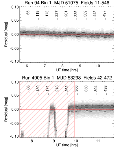
Figure 9.— Magnitude residuals as a function of time/field number for two example runs; all six camera columns are combined in these plots. The contours again show the 25%, 50%, and 75% levels. The red hatched regions mark periods of time independently known to be non-photometric from the SDSS photometricity monitors. Note that both these runs are on the multiply imaged Equatorial stripe, and therefore have lots of overlaps. However, for a large fraction of the data, the overlaps are considerably more sparse.

Finally, we plot the magnitude residuals, grouped by run, as a function of field number (and time); two examples are in Fig. 9. These plots are our primary diagnostic of the photometricity of the data. Photometric data have the mean residual scattered around zero, although often with coherent errors at the few millimagnitude level. By contrast, the residuals for unphotometric data show large excursions from zero, often at the $\sim 10\%$ level or greater. Most of these data have already been correctly flagged as being non-photometric by the SDSS photometricity monitors (Hogg et al., 2001) and have been excluded from the solution. Any remaining non-photometric data is manually flagged as such, and removed in a second iteration of the calibration. For all the non-photometric data that overlaps photometric data, we can estimate an a-term per field that minimizes the residuals which determines the calibration of those fields (these are still flagged as being non-photometric).

5.2. Spatial Error Modes

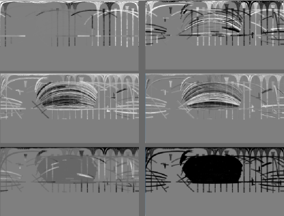
Figure 10.— Examples of the spatial structure in the calibration errors for the $r$ band, organized from left to right, and top to bottom in increasing order of their uncertainties. The top left mode is the best constrained, while the bottom right mode is the worst constrained. The middle row are examples of modes with typical errors. The modes are normalized such that the maximum absolute error is 1. Note that the worst constrained mode is the exactly degenerate overall zeropoint of the survey. The structures are similar for the other bands.

Since our goal in this paper is accurate relative calibration, it behooves us to understand the spatial structure in the calibration errors. Our starting point is the curvature matrix, Eq. 27. The eigenvectors of this matrix partition our basis of photometric parameters into uncorrelated linear combinations, whose uncertainties are given by the inverses of the corresponding eigenvectors. An error in each photometric parameter can be thought of as a pattern of errors on the sky, determined by the runs corresponding to that parameter. One can use this to project the eigenvectors (modes) of the curvature matrix on the sky. These then describe the spatial structure of the calibration errors (Fig. 10). Note that projecting these modes on the sky destroys the linear independence of the modes; if desired, this can be restored by a straightforward orthogonalization.

The worst constrained mode is, as expected, the zero point of the calibration which is exactly degenerate. However, examining the other poorly constrained modes (an example of which is the bottom left of Fig. 10), we observe that there are no other such simple large scale modes, an indication of the fact the survey is well connected. At the other extreme are the best constrained modes. These are typically complicated combinations, and not surprisingly describe modes held together by the grid of Apache Wheel data. More illuminating are examples of typical modes, two of which are in the middle row of Fig. 10. The most noticeable characteristic is the striping along the scan direction. This simply reflects the fact that we calibrate camera columns individually, resulting in errors correlated in the scan direction.

We do not fit for $dk/dt$, and so it does not get included in the curvature matrix. However, we saw in Sec. 4.1 that it resulted in a coherent tilt from one end of the survey to the other.

5.3. Experimental Stability

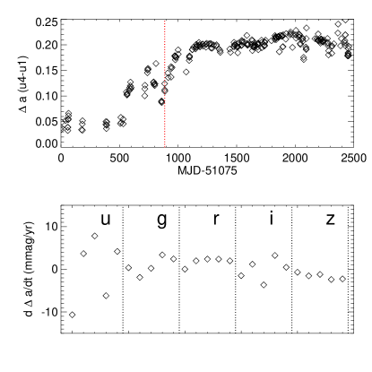
Figure 11.— [top] The difference between the a-terms of $u$ band camera column 4 and 1; since the atmospheric corrections are common to both of these, this is a measure of the stability of the telescope + camera system. The drift in the camera during early data due to problems with the vacuum system (see Table 1) is clearly visible; the vertical dotted line at MJD 51960 marks when the vacuum system was fixed. Note that all of the changes are long term drifts; the system is stable on short (i.e. day) intervals as assumed in our model. [bottom] The drift in the relative (to camera column 1) zero points of camera columns 2 through 6, for all five filters in mmag/year, measured after MJD 51960.

Our results for the photometric calibration can also be used to estimate the overall photometric stability of the SDSS camera, telescope and site. We estimate the camera stability by considering differences between a-terms as a function of time (for definiteness, we compute the a-terms relative to camera column 1); these differences are insensitive to any common mode effects (such as the atmosphere). An example is in Fig. 11. During the initial phases of the survey, we note that the camera was not very stable over long time periods, reflecting various problems with the vacuum system flagged in Table 1. However, over the past $\sim 5$ years, the camera has been extremely stable, as evidenced by an overall drift in the a-term differences of $<\sim 10$ mmag/yr, for all the CCDs.

One could also measure the combined stability, treating the camera, telescope, and site as a combined system. As the a- and k-terms are degenerate, we consider the combination $a-k\langle x\rangle$ every night, where we average the airmass over all the observations in a given night. This is plotted in Fig. 12 for the five SDSS filters. The most striking aspect of these data are the seasonal variations, seen as periodic oscillations in the data, at the $\sim 10\%$ level (except in the $u$ band, where they are $\sim 20\%$). Factoring out the seasonal variations, we find less than a 5% drift over the $\sim 7$ years considered here (again, except the $u$ band, where the drift is $\sim 10\%$ over the same time period).

Figure 12.— The value of $a-k\langle x\rangle$ for camera column 1 as a function of MJD, and filter; $\langle x\rangle$ is the mean airmass of all the observations in a given night. This combination is insensitive to degeneracies between the a- and k-terms, and measures the overall photometric stability of the SDSS camera, telescope and site. The seasonal variations in these data are clearly apparent, as is the fact that the mirror is aluminized every summer.

We emphasize that all of the effects discussed here are long-term effects and do not affect the quality of the calibration which only assumes stability over a night for the a- and k-terms.

5.4. Principal colors

The above discussion has relied on a combination of simulations and internal consistency checks to assess the quality of the calibrations. While these provide essential perspectives, they have important disadvantages as well. Internal consistency checks are not independent of the calibration and might not flag deviations from the input model. Furthermore, these checks are local measurements, and do not provide information about large scale systematics problems. While simulations fill that gap, they are limited by the input model used. Astrophysical tests complement the above by providing large scale, independent verification, and are ultimately limited by astrophysical uncertainties.

The majority ($>\sim 98\%$) of the stars detected by the SDSS are on the main sequence (Finlator et al., 2000; Helmi et al., 2003), and lie on one-dimensional manifolds (the “stellar locus”) on color-color diagrams. This suggests using the position of the stellar locus as a diagnostic of calibration errors (Ivezić et al., 2004). While there are a number of morphological features one could use as a marker, we follow the discussion in Ivezić et al. (2004) and use the “principal colors” that define directions perpendicular to the stellar locus. We consider four such colors (Ivezić et al., 2004) : $s$ (perpendicular to the blue part of the locus in $u-g$ vs. $g-r$ plane), $w$ (the blue part in $g-r$ vs. $r-i$), $x$ (the red part in $g-r$ vs. $r-i$), and $y$ (the red part in $r-i$ vs. $i-z$):

$$s = -0.249u+0.794g-0.555r+0.234$$

$$w = -0.227g+0.792r-0.567i+0.050$$

$$x = 0.707g-0.707r-0.988$$

$$y = -0.270r+0.800i-0.534z+0.054\,\,.$$ (30)

We correct all magnitudes with the Schlegel et al. (1998) estimates of extinction (except immediately below), but do not attempt any correction for stars not completely behind all the dust. Since we calibrate each band separately, and apply no color cuts to select the stars used, the above principal color diagnostics provide a completely independent verification of the calibration.

Fig. 13 plots these on a $\mu$-stripe projection; the $x$-direction is the coordinate along the scan direction $\mu$ (Pier et al., 2003), while the $y$ coordinate is given by

$$y =12({\rm stripe})+2({\rm camcol})-2\,, {\rm strip=S}$$ (31)

$$=12({\rm stripe})+2({\rm camcol})-1\,, {\rm strip=N}\,\,,$$

where stripe, strip and camcol is the SDSS stripe number, whether it is a northern or southern strip, and the camera column respectively. This lays out each camera column as a row, respecting the interleaved structure of the strips within a stripe. The advantage of this projection is that calibration errors appear principally as stripes in the $\mu$ direction, while Galactic structure appears as irregular structures localized in $\mu$, making it easier to separate the two. For the purpose of this plot, we use colors not corrected for extinction to highlight the Galactic structure. We simply exclude the small fraction of data not on survey stripes for the purposes of this analysis.

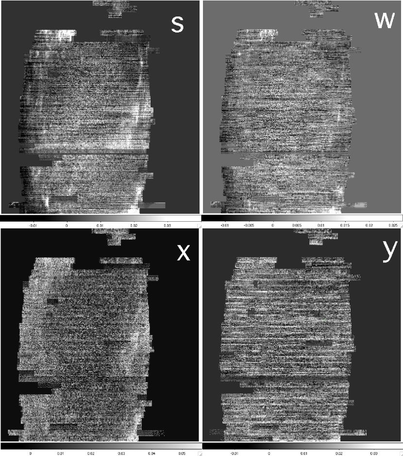
Figure 13.— The spatial variation in the $s$ (top left), $w$ (top right), $x$ (bottom left), and $y$ (bottom right) principal stellar colors. The projection is a $\mu-$stripe projection, with the $x$ coordinate measuring $\mu$ (the coordinate along the scan direction). The $y$ coordinate is the SDSS stripes, with each row as one of the 12 camera columns that define the stripe. We have restricted ourselves to data on survey stripes between 9 and 44, corresponding to most of the North Galactic cap, in this plot. Note that the aspect ratio in the $\mu$ direction is significantly compressed.

We note that there is little visual evidence for any striping over the entire survey region in $s$, $w$, and $x$. Reddening from Galactic dust is clearly visible in $s$ and $x$, which are colors nearly parallel to the reddening vector. The $y$ map, on the other hand, does appear to show striping, with a periodicity on the SDSS stripe scale. In order to quantify this effect, we plot the average principal color per camera column (distinguishing between northern and southern strips) in Fig. 14. As anticipated from the 2D maps, the $s$, $w$, and $x$ colors are uniform at the $0.5\%$ (peak to peak) level, whereas camera column 2 is offset in $y$ at 0.7% (peak to peak). It is unlikely that this is an artifact of the calibration process which treats all camera columns identically. Since $y$ is the only color to use the $z$ band, we speculate that this could be caused by the known variations in the $z$-band filter responses. However, as this effect is of the same order as other systematics present in the calibration (and below our target of 1%), we simply caution the reader about this systematic in this paper, and defer its resolution to future work.

Figure 14.— The average principal colors measured for each of the 6 camera columns, for the north and south strips separately. As before, we restrict ourselves to stripes between 9 and 44. The mean color has been subtracted from each of the four curves; the means are -0.002, 0.004, 0.007 and 0.007 for $s$, $w$, $x$ and $y$ respectively. The variations between camera columns are $<1\%$ (peak to peak) for all colors.

The above has focused on large scale systematics; Fig. 15 shows examples of the principal colors as a function of CCD column averaging over a random sample of runs in a flat field season. The deviations from a constant color are $\mbox{${}^{<}_{\sim}$}1\%$ for all colors, and $<0.5\%$ for $s$ and $w$, consistent with our estimates from simulations. We also observe errors in the amp-jump determination at the $\sim 0.5\%$ level, similar to Fig. 8.

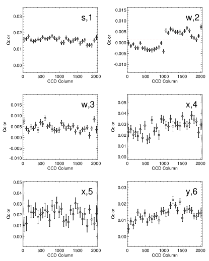
Figure 15.— Examples of the principal colors as a function of CCD column. The principal color and camera column used is noted in each panel. Each panel plots a color measured over a group of runs, chosen to be in the same flatfield season (Table 1). From 1 through 6, the runs used are (745, 752,756),(1331,1345),(2190, 2299),(2566, 2662, 2883, 2886), (3560, 3830) and (4927, 5052) respectively. Deviations in the color from a constant (dotted line) indicate errors in the flatfield determination.

5.5. Comparison with previous results

We conclude this section by comparing the calibrations presented here with those publicly available as part of Data Release 4 (Adelman-McCarthy et al., 2006, DR4) . Fig. 16 shows the difference between the aperture magnitudes of DR4 and those derived in this paper, for all stars with $r$ band magnitude less than 18. The magnitudes agree on average by construction, as the zero points were determined by matching to the public calibration. Furthermore, the scatter is approximately 2% (r.m.s) for $griz$, and 3% (r.m.s) in $u$, consistent with the published uncertainties. The Data Release errors are therefore dominated by the Photometric Telescope (PT) based calibration method.

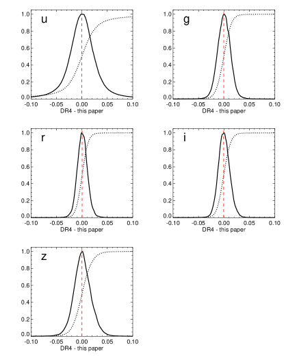
Figure 16.— Histograms of the differences in magnitudes between DR4 and this work, for stars with $r$-band magnitudes $<$ 18.0. Shown are the distribution of differences (normalized to have a maximum value of 1), as well as the cumulative distibution (dotted line). The vertical lines show the median of the distribution, which is $<0.001$ mag for all five filters.

Fig. 17 plots these differences in the $\mu$-stripe projection introduced previously. Since the standard SDSS calibration does not attempt to explicitly control relative calibration errors, the striping in the figure is not surprising. Note that the errors are correlated in the $\mu$ direction as expected, but also across camera columns. The latter arises from the fact that the calibration patches are 40’ wide and span three camera columns, thereby correlating their calibrations.

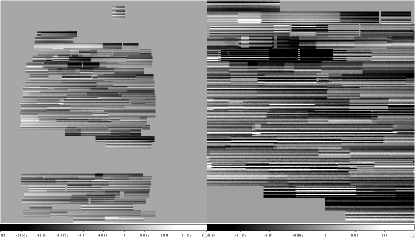
Figure 17.— The difference in magnitudes between DR4 and this work in the $r$ band for the stars in Fig. 16, plotted in the $\mu$-stripe projection. The right panel zooms in to a region to highlight the structure in the calibration errors.

Finally, Fig. 18 plots the differences in the DR4 flat fields, and those determined in this paper, for an example flat field season. The errors in the flat fields are both higher than the quoted uncertainties and appear to have long wavelength power. We speculate that these result from the method used to determine the flux response of the CCDs, which aliases flat field errors in the Photometric Telescope into the final flat fields. This aliasing is mitigated by using the average of $g$,$r$, and $i$, instead of any of those bands individually; this does not however eliminate the problem. Formally, these errors are $\sim 1\%$ (r.m.s.), but are highly correlated, both spatially and in color.

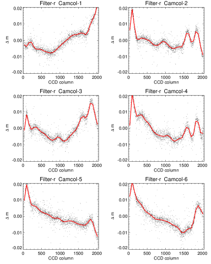
Figure 18.— The difference between the $r$ band DR4 flat fields and those determined in this work, for SDSS runs between 4100 and 4400. These differences are traced by the difference in magnitudes as a function of CCD column, for the 6 camera columns. The solid line shows the median difference, while the points are a subsampling of the individual measurements. We restrict ourselves to runs between 4100 and 4400 to select runs within a single flat field season.

6. Public Data Release

The calibrations (dubbed “ubercalibration”) described in this work have been made public with the SDSS Data Release 6 , and will be updated for the subsequent data releases. The SDSS Catalog Archive Server has recalibrated versions of the most popular magnitudes, as well as correction terms that can be applied to other magnitudes. We refer the reader to the documentation under “ubercalibration” on the SDSS data release websites for the most up-to-date information on these calibrations, and the available data formats.

7. Discussion

We have presented a method for calibrating wide field imaging surveys using overlaps in observations, and applied it to the Sloan Digital Sky Survey imaging. Early versions of these calibrations have already been used for the creation of a number of auxiliary SDSS catalogs (e.g. Finkbeiner et al., 2004; Blanton et al., 2005) as well as a number of SDSS scientific publications (e.g. Tegmark et al., 2004; Eisenstein et al., 2005; Padmanabhan et al., 2007; Tegmark et al., 2006).

The principal features and results of this work are :

• Relative vs. Absolute Calibrations: We explicitly separate the problem of relative calibrations from that of absolute calibration. The problem of absolute calibrations then reduces to determining one zeropoint per filter for the entire survey (however, see the caveat on spectral energy distributions below), and does not alias into spatial variations in the calibration. This allows us to better control and quantify the errors in the relative calibration.

• Simulations : We emphasize the utility of simulations, both to validate pipelines, and to quantify the structure in the calibration errors. Simple analytical estimates are insufficient to characterize the errors, while astrophysical estimates are limited by their intrinsic scatter. Developing realistic simulations for the next generation of surveys must be an essential part of any calibration pipeline. Such simulations also are invaluable in determining the observing strategy (before any data are actually taken) that yields the desired calibration accuracy.

• Stellar Flat Fields : The problems of flat fielding wide field-of-view instruments, namely (i) non-uniform illumination for dome flats, (ii) spatial gradients and scattered light for sky flats and (iii) mismatched spectral energy distributions (SEDs) have been discussed extensively in the literature (e.g. Manfroid, 1995; Chromey & Hasselbacher, 1996; Magnier & Cuillandre, 2004; Stubbs & Tonry, 2006). In particular, initial attempts to use sky flats for the SDSS resulted in errors of 5% in the $r$ band and as bad as 20% in the $u$ band, due to scattered light within the instrument. These were therefore never used for the public data; instead the published SDSS flat fields are determined from the position of the stellar locus. The use of stellar flat fields mitigates all three of these (Manfroid, 1995). Given sufficient observations and overlaps, one has sufficient S/N to map out the entire flat field with high precision. Furthermore, since one is using a realistic ensemble of stars by construction, biases due to differences between the flat field SED and the SED of a given object are minimized. Note that there are still potential biases for objects of unusual color; these cannot however be treated in a general manner.

• 1% Relative Calibrations/Spatial Error Modes : Our recalibrated SDSS imaging data has relative calibration errors, determined from simulations, of $\sim$ 13, 8, 8, 7, and 8 mmag in $ugriz$ respectively. We however do detect systematics not modeled in our simulations at the $\sim 0.5$% level, suggesting a conservative estimate of $1\%$ errors in $griz$ and $2\%$ in $u$. In addition, we are able to characterize the spatial structure of the errors as a combination of error modes. Most of these modes show little coherent spatial structure. The most significant spatial structure results from misestimating the time variation of the k-terms, which introduces a tilt into the survey.

Throughout this paper, we ignored a number of sub-dominant systematic effects. We briefly discuss these below, both to document their existence as well as to alert future surveys of potential pitfalls.

• Spectral Energy Distributions: When interpreting our magnitudes as absolute, our algorithm implicitly assumes that all objects have the same spectral energy distribution. The median $r-i$ color of stars used in the calibration is $\sim 0.2$, and we expect the calibrations to be accurate (at the stated levels) for objects with colors not very different from these stars. This will however not be true for objects with unusual SEDs (e.g. SNe). In these cases, one must integrate the SED over the system response, in order to get an absolute, calibrated flux $(\rm{inerg\,cm}^{-2}\rm{s}^{-1})$.

• Filter Curves: We assume that the six copies of each filter are identical, and do not attempt any color corrections between the six camcols. We verified the validity of this assumption by generating synthetic $ugriz$ photometry for the Gunn-Stryker spectra (Gunn & Stryker, 1983) for each of the six camcols, using the individually measured filter curves. For stars with median $r-i$ color close to $\sim 0.2$, the differences between the various camcols was better than $1\%$ for $griz$ and $\sim 1\%$ for the $u-$band. Of $griz$, the most drastic variation with color occurs for the $z-$band, with a $0.01$ mag gradient between $r-i=0$ and $1$ seen is almost all the camcols. Gradients of a similar magnitude are also seen for $g2$, $g4$ and $r3$.

• Absolute Calibrations: We ignored the issues of determining the absolute calibration (i.e. the five zero-points) of the SDSS system, choosing instead to have it agree with the published SDSS magnitudes. In particular, any corrections to put the SDSS system on to the AB system also apply in our case.

We conclude by discussing how to extend the program presented here to the next generation of imaging surveys. Our starting point will be the second distinction made in Sec. 1 - separating the telescope and the atmosphere explicitly in the calibrations. It is relatively straightforward to adapt the algorithm presented here to use high precision measurements of the telescope response functions as a starting point; these would be analogous to the priors already considered here.

Understanding atmospheric variations is an important step towards 1% photometry; unmodeled variations are responsible for almost all our calibration error budget. These transparency variations are dominated by three well-studied processes (Hayes & Latham, 1975): Rayleigh scattering, molecular absorption by ozone (dominant in the UV) and water vapor (dominant in the red and IR), and aerosol scattering. Of these, Rayleigh scattering is best understood, and is well determined by the local atmospheric pressure. While absorption and aerosol scattering are well understood in an average sense, their time variation is significant. Tracking these would therefore require continuous monitoring of the atmosphere, plus detailed atmospheric models. The payback for doing so would be a dramatic reduction in calibration errors.

The algorithm we propose in this paper demonstrates that 1% relative photometry is achievable by the current generation of wide field imaging surveys. The challenge for the next generation of surveys is to break through the 1% barrier.

NP is supported by a NASA Hubble Fellowship HST-HF-01200.

Funding for the SDSS and SDSS-II has been provided by the Alfred P. Sloan Foundation, the Participating Institutions, the National Science Foundation, the U.S. Department of Energy, the National Aeronautics and Space Administration, the Japanese Monbukagakusho, the Max Planck Society, and the Higher Education Funding Council for England. The SDSS Web Site is http://www.sdss.org/.

The SDSS is managed by the Astrophysical Research Consortium for the Participating Institutions. The Participating Institutions are the American Museum of Natural History, Astrophysical Institute Potsdam, University of Basel, Cambridge University, Case Western Reserve University, University of Chicago, Drexel University, Fermilab, the Institute for Advanced Study, the Japan Participation Group, Johns Hopkins University, the Joint Institute for Nuclear Astrophysics, the Kavli Institute for Particle Astrophysics and Cosmology, the Korean Scientist Group, the Chinese Academy of Sciences (LAMOST), Los Alamos National Laboratory, the Max-Planck-Institute for Astronomy (MPIA), the Max-Planck-Institute for Astrophysics (MPA), New Mexico State University, Ohio State University, University of Pittsburgh, University of Portsmouth, Princeton University, the United States Naval Observatory, and the University of Washington.

References

- Abazajian et al. (2005) Abazajian, K., et al. 2005, AJ, 129, 1755
- Abazajian et al. (2004) Abazajian, K., et al. 2004, AJ, 128, 502
- Abazajian et al. (2003) Abazajian, K., et al. 2003, AJ, 126, 2081
- Adelman-McCarthy et al. (2007) Adelman-McCarthy, J. K., et al. 2007, ApJS, 172, 634
- Adelman-McCarthy et al. (2006) Adelman-McCarthy, J. K., et al. 2006, ApJS, 162, 38
- Adelman-McCarthy & for the SDSS Collaboration (2007) Adelman-McCarthy, J. K., & for the SDSS Collaboration. 2007, ApJS. submitted (astro-ph/0707.3413)
- Alcock et al. (1993) Alcock, C., et al. 1993, Nature, 365, 621
- Aubourg et al. (1993) Aubourg, E., et al. 1993, Nature, 365, 623
- Bessell (2005) Bessell, M. S. 2005, ARA&A, 43, 293
- Blake et al. (2007) Blake, C., Collister, A., Bridle, S., & Lahav, O. 2007, MNRAS, 374, 1527
- Blanco et al. (1987) Blanco, V. M., et al. 1987, ApJ, 320, 589
- Blanton et al. (2005) Blanton, M. R., et al. 2005, AJ, 129, 2562
- Chromey & Hasselbacher (1996) Chromey, F. R., & Hasselbacher, D. A. 1996, PASP, 108, 944
- Eisenstein et al. (2005) Eisenstein, D. J., et al. 2005, ApJ, 633, 560
- Finkbeiner (2004) Finkbeiner, D. P. 2004, ApJ, 614, 186
- Finkbeiner et al. (2004) Finkbeiner, D. P., et al. 2004, AJ, 128, 2577
- Finlator et al. (2000) Finlator, K., et al. 2000, AJ, 120, 2615
- Fong et al. (1992) Fong, R., Hale-Sutton, D., & Shanks, T. 1992, MNRAS, 257, 650
- Fong et al. (1994) Fong, R., Metcalfe, N., & Shanks, T. 1994, in IAU Symp. 161: Astronomy from Wide-Field Imaging, ed. H. T. MacGillivray, 295
- Fukugita et al. (1996) Fukugita, M., Ichikawa, T., Gunn, J. E., Doi, M., Shimasaku, K., & Schneider, D. P. 1996, AJ, 111, 1748
- Glazebrook et al. (1994) Glazebrook, K., Peacock, J. A., Collins, C. A., & Miller, L. 1994, MNRAS, 266, 65
- Górski et al. (1999) Górski, K. M., Hivon, E., & Wandelt, B. D. 1999, in Evolution of Large Scale Structure : From Recombination to Garching, 37
- Gunn et al. (1998) Gunn, J. E., et al. 1998, AJ, 116, 3040
- Gunn et al. (2006) Gunn, J. E., et al. 2006, AJ, 131, 2332
- Gunn & Stryker (1983) Gunn, J. E., & Stryker, L. L. 1983, ApJS, 52, 121
- Hayes & Latham (1975) Hayes, D. S., & Latham, D. W. 1975, ApJ, 197, 593
- Helmi et al. (2003) Helmi, A., et al. 2003, ApJ, 586, 195
- Hogg et al. (2001) Hogg, D. W., Finkbeiner, D. P., Schlegel, D. J., & Gunn, J. E. 2001, AJ, 122, 2129
- Honeycutt (1992) Honeycutt, R. K. 1992, PASP, 104, 435
- Ivezić et al. (2007) Ivezić, Ž., Allyn Smith, J., Miknaitis, G., Lin, H., & Tucker, D. 2007, AJ submitted (astro-ph/0703157)
- Ivezić et al. (2004) Ivezić, Ž., et al. 2004, Astronomische Nachrichten, 325, 583
- Juric et al. (2005) Juric, M., et al. 2005, ApJ submitted (astro-ph/0510520)
- Landolt (1983) Landolt, A. U. 1983, AJ, 88, 439
- Landolt (1992) Landolt, A. U. 1992, AJ, 104, 340
- Lupton et al. (2001) Lupton, R. H., Gunn, J. E., Ivezić, Z., Knapp, G. R., Kent, S., & Yasuda, N. 2001, in ASP Conf. Ser. 238: Astronomical Data Analysis Software and Systems X, 269
- Maddox et al. (1990) Maddox, S. J., Efstathiou, G., & Sutherland, W. J. 1990, MNRAS, 246, 433
- Magnier & Cuillandre (2004) Magnier, E. A., & Cuillandre, J.-C. 2004, PASP, 116, 449
- Manfroid (1993) Manfroid, J. 1993, A&A, 271, 714
- Manfroid (1995) Manfroid, J. 1995, A&AS, 113, 587
- Oke & Gunn (1983) Oke, J. B., & Gunn, J. E. 1983, ApJ, 266, 713
- Padmanabhan et al. (2007) Padmanabhan, N., et al. 2007, MNRAS, 378, 852
- Pier et al. (2003) Pier, J. R., Munn, J. A., Hindsley, R. B., Hennessy, G. S., Kent, S. M., Lupton, R. H., & Ivezić, Ž. 2003, AJ, 125, 1559
- Pont et al. (2006) Pont, F., Zucker, S., & Queloz, D. 2006, MNRAS, 373, 231
- Press et al. (1992) Press, W. H., Teukolsky, S. A., Vetterling, W. T., & Flannery, B. P. 1992, Numerical recipes in FORTRAN. The art of scientific computing (Cambridge University Press, 1992, 2nd ed.)
- Schlegel et al. (1998) Schlegel, D. J., Finkbeiner, D. P., & Davis, M. 1998, ApJ, 500, 525
- Smith et al. (2002) Smith, J. A., et al. 2002, AJ, 123, 2121
- Stoughton et al. (2002) Stoughton, C., et al. 2002, AJ, 123, 485
- Stubbs & Tonry (2006) Stubbs, C. W., & Tonry, J. L. 2006, ApJ, 646, 1436
- Tegmark (1997) Tegmark, M. 1997, ApJ, 480, L87
- Tegmark et al. (2004) Tegmark, M., et al. 2004, ApJ, 606, 702
- Tegmark et al. (2006) Tegmark, M., et al. 2006, Phys. Rev. D, 74, 123507
- Tucker et al. (2006) Tucker, D. L., et al. 2006, Astronomische Nachrichten, 327, 821
- Udalski et al. (1992) Udalski, A., Szymanski, M., Kaluzny, J., Kubiak, M., & Mateo, M. 1992, Acta Astronomica, 42, 253
- York et al. (2000) York, D. G., et al. 2000, AJ, 120, 1579