CosmoNet: fast cosmological parameter estimation in non-flat models using neural networks

Abstract

We present a further development of a method for accelerating the calculation of CMB power spectra, matter power spectra and likelihood functions for use in cosmological Bayesian inference. The algorithm, called CosmoNet, is based on training a multilayer perceptron neural network. We demonstrate the capabilities of CosmoNet by computing CMB power spectra (up to $\ell=2000$) and matter transfer functions over a hypercube in parameter space encompassing the $4\sigma$ confidence region of a selection of CMB (WMAP + high resolution experiments) and large scale structure surveys (2dF and SDSS). We work in the framework of a generic 7 parameter non-flat cosmology. Additionally we use CosmoNet to compute the WMAP 3-year, 2dF and SDSS likelihoods over the same region. We find that the average error in the power spectra is typically well below cosmic variance for spectra, and experimental likelihoods calculated to within a fraction of a log unit. We demonstrate that marginalised posteriors generated with CosmoNet spectra agree to within a few percent of those generated by CAMB parallelised over 4 CPUs, but are obtained 2-3 times faster on just a single processor. Furthermore posteriors generated directly via CosmoNet likelihoods can be obtained in less than 30 minutes on a single processor, corresponding to a speed up of a factor of $\sim 32$. We also demonstrate the capabilities of CosmoNet by extending the CMB power spectra and matter transfer function training to a more generic 10 parameter cosmological model, including tensor modes, a varying equation of state of dark energy and massive neutrinos. Finally we demonstrate that using CosmoNet likelihoods directly, the sampling strategy adopted by CosmoMC is highly sub-optimal. We find the generic Bayesys sampler (Skilling, 2004) sampler to be a further $\sim 10$ times faster, yielding 20,000 post burn-in samples in our 7 parameter model in just 3 minutes on a single CPU. CosmoNet and interfaces to both CosmoMC and Bayesys are publically available at www.mrao.cam.ac.uk/software/cosmonet.

1 Introduction

Bayesian inference in cosmology is normally carried out using sampling based methods as now required by the dimensionality of the models and increasingly high-precision of the data sets. Typically one requires the calculation of theoretical temperature and polarisation CMB power spectra $C_{\ell}^{\rm TT}$, $C_{\ell}^{\rm TE}$, $C_{\ell}^{\rm EE}$ and $C_{\ell}^{\rm BB}$ and/or the matter power spectrum $P(k)$ using codes such as CMBfast (Seljak & Zaldarriaga, 1996) or CAMB (Lewis et al., 2000). These codes typically require of order 10 secs for spatially-flat models and 50 secs for non-flat models on a 2 GHz CPU. This approach is therefore computationally demanding, but does have the advantage that it is simple to generalise if one wishes to include new physics. CosmoMC (Lewis & Bridle, 2002) currently represents the state of the art in cosmological Markov Chain Monte Carlo (MCMC) sampling and employs a number of strategies to improve performance, such as a division of the parameter space into ‘slow’ parameters (which determine the evolution of structure) and ‘fast’ parameters which determine the primordial power spectrum. Nonetheless, the technique is still computationally expensive.

A number of examples exist in the literature of methods reliant on generating (to some degree or other) grids of models, within which various interpolations are made to compute observable spectra at arbitrary parameter values. One example is Dash (Kaplinghat et al., 2002) which requires a considerable investment of some 40 hours to generate a grid of transfer functions which can then be used to generate $C_{\ell}$ spectra for a given parameter combination about $30$ times faster than CAMB.

Jimenez et al. (2004) have built a less demanding method around the novel idea of transformation into the mostly uncorrelated physical parameterisation introduced by Kosowsky et al. (2002). Since the $C_{\ell}$’s have a simple dependence on the input parameters they are then relatively easy to model. The algorithm, known as CMBwarp then uses polynomials to fit the spectra in which the polynomial coefficients are tied to the spectra at some, single point in the parameter space. This allows spectra to be generated $\sim 3000$ times faster than CAMB. Of course this method suffers from the drawback that the single model about which the polynomial fit is specified must be chosen carefully to lie close to the centre of the posterior distribution as accuracy decreases away from this point. Within a $3\sigma$ region around the chosen model they estimate it gives better than 1% accuracy.

The advent of larger datasets have meant the time spent calculating model likelihoods is rapidly approaching the time necessary to generate the theoretical spectra. CMBfit (Sandvik et al., 2004) proposes to remove the step of determining spectra altogether by providing a semi-analytic fit directly to the WMAP likelihood as a function of input cosmological parameters. Given the ubiquity of WMAP data in cosmological analyses the drawback of being tied to a single experiment is however not as limiting as one might think.

The methods just described, although useful, lack general applicability over a range of theoretical spectra and datasets. We have been motivated to generate a new method that can be applied, almost blindly to the problem of cosmological inference in order to remove the two largest bottlenecks of theoretical spectra generation and likelihood evaluation. Previously Fendt & Wandelt (2007) built a robust new method based on machine-learning called Pico. Their method requires the assembly of $\sim 10^{4}$ samples over the parameter space drawn uniformly from a desired region that could encompass any confidence region of a given experiment. This ‘training set’ is compressed via a principal component analysis (using Karhunen–Loève eigenmodes) which typically results in a reduction in the dimensionality of the training set by a factor of two. The training set is used to divide the parameter space into ($\sim 100$) regions using $k$-means clustering (see e.g. MacKay 1997) with the aim of each cluster encompassing a region of parameter space over which the power spectra vary equally. A polynomial fit is then used over each cluster providing a local interpolation of the power spectra within the cluster as a function of cosmological parameters. Crucially, the method fails to model the spectra accurately over the entire parameter space, hence the need for cluster division and thus making the algorithm difficult to extend.

Both Pico and CMBWarp provide similar improvements in efficiency, but Pico is an order of magnitude more accurate than both DASh and CMBWarp. It is generic enough to be extended to any observable spectra and is flexible enough to allow prediction of likelihood values, thus incorporating the benefits made by the CMBfit code. Given the current speed of the WMAP 3-year likelihood [Hinshaw et al. (2006), WMAP3] code this particular facet of the method will become extremely important in future analyses.

We previously presented (Auld et al., 2007) a new method that combined all of the advantages of Pico but in a simpler and more readily expandable form by training neural networks. The resulting algorithm is called CosmoNet and has some considerable additional benefits in terms of the scalability, accuracy and computational memory requirements. In addition, the training method we employ is sufficiently general and simple to apply that it allows the end user to generate their own trained nets over any chosen cosmological model. In this paper we extend the method to include more generic (non-flat) cosmological models, interpolations over matter transfer functions and two large scale structure likelihoods in addition to the suite of CMB power spectra and the WMAP3 likelihood. Additionally we extend the $\ell$ range of our CMB spectra interpolation to $\ell_{\rm max}=2000$. In Sec. 2 we briefly describe neural networks. In Sec. 3 we describe the CosmoNet algorithm and training efficiency. In Sec. 4 we present cosmological parameter estimates using the trained networks implemented as CosmoNet. In Sec. 5, we apply the CosmoNet training algorithm to a 10 parameter cosmological model, training the CMB power spectra and matter transfer functions and producing parameter estimates. Our discussions and conclusions are presented in Sec. 6.

2 Neural network interpolation

Neural networks are a methodology for computing loosely based around the structures found in animal brains. They consist of a number of interconnected processors called neurons. The neurons process information separately and pass information to one another via connections. Well-designed networks are able to ‘learn’ from training data and are able to make predictions when presented with new, possible incomplete, information. For an introduction to the science of neural networks the reader is directed to Bailer-Jones (2001).

2.1 Multilayer perceptron networks

The perceptron (Rosenblatt, 1958) is the simplest type of feed-forward neural network. It maps an input vector $\mathbf{x}\in\Re^{n}$ to a scalar output $f(\mathbf{x};\mathbf{w},\theta)$ via

$$f(\mathbf{x};\mathbf{w},\theta)=\sum_{i}w_{i}x_{i}+\theta,$$ (1)

where $\{w_{i}\}$ and $\theta$ are the parameters of the perceptron, called the ‘weights’ and ‘bias’ respectively.

Multilayer perceptron neural networks (MLPs) are a type of feed-forward network composed of a number of ordered layers of perceptron neurons that pass scalar messages from one layer to the next. In this paper, we will work with 3-layer MLPs only. They consist of an input layer, a hidden layer and an output layer (Fig. 1). In such a network, the outputs of the nodes in the hidden and output layers take the form

hidden layer: $$h_{j}=g^{(1)}(f_{j}^{(1)}); f_{j}^{(1)}=\sum_{l}w^{(1)}_{jl}x_{l}+\theta_{j}^{(1)},$$ (2)

output layer: $$y_{i}=g^{(2)}(f_{i}^{(2)}); f_{i}^{(2)}=\sum_{j}w^{(2)}_{ij}h_{j}+\theta_{i}^{(2)},$$ (3)

where the index $l$ runs over input nodes, $j$ runs over hidden nodes and $i$ runs over output nodes. The functions $g^{(1)}$ and $g^{(2)}$ are called activation functions and are chosen to be bounded, smooth and monotonic. In this paper, we use $g^{(1)}(x)=\tanh x$ and $g^{(2)}(x)=x$, where the non-linear nature of the former is a key ingredient in constructing a viable network.

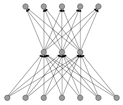
Figure 1: An example of a 3-layer neural network with seven input nodes, 3 nodes in the hidden layer and five output nodes. Each line represents one weight.

The weights $\mathbf{w}$ and biases $\mathbf{\theta}$ are the quantities we wish to determine, which we denote collectively by $\mathbf{a}$. As these parameters vary, a very wide range of non-linear mappings between the inputs and outputs are possible. In fact, according to a ‘universal approximation theorem’ (Leshno et al. 1993), a standard multilayer feed-forward network with a locally bounded piecewise continuous activation function can approximate any continuous function to any degree of accuracy if (and only if) the network’s activation function is not a polynomial. This result applies when activation functions are chosen apriori and held fixed as $\mathbf{a}$ varies. Accuracy increases with the number in the hidden layer and the above theorem tells us we can always choose sufficient hidden nodes to produce any accuracy. Since the mapping from cosmological parameter space to the space of CMB power spectra (and WMAP3 likelihood) is known to be continuous, a 3-layer MLP with an appropriate choice of activation function is an excellent candidate model for the replacement of the forward model provided by the CAMB package (and WMAP3 likelihood code).

The activation functions act as basic building blocks of non-linearity in a neural network model and should be as simple as possible. Additionally, the MemSys routines used in training (described below) require derivative information and so they should be differentiable. The universal approximation theorem thus motivates us to choose a monotonic (for simplicity), bounded and differentiable function that is not a polynomial and we choose the $\tanh$ function. Of course, this could be replaced by another such function, such as the sigmoid function, but the interpolation results would be almost identical.

2.2 Network training

Let us consider building an empirical model of the CAMB mapping using a 3-layer MLP as described above (a model of the different likelihood codes can be constructed in an analogous manner). The number of nodes in the input layer will correspond to the number of cosmological parameters, and the number in the output layer will be the number of uninterpolated $C_{\ell}$ values output by CAMB. A set of training data ${\cal{D}}=\{\mathbf{x}^{(k)},\mathbf{t}^{(k)}\}$ is provided by CAMB (the precise form of which is described later) and the problem now reduces to choosing the appropriate weights and biases of the neural network that best fit this training data.

As the CAMB mapping is exact, this is a deterministic problem, not a probabilistic one. We therefore wish to choose network parameters $\mathbf{a}$ that minimise the ‘error’ term $\chi^{2}(\mathbf{a})$ on the training set given by

$$\chi^{2}(\mathbf{a})=\frac{1}{2}\sum_{k}\sum_{i}\left[t^{(k)}_{i}-y_{i}(\mathbf{x}^{(k)};\mathbf{a})\right]^{2}.$$ (4)

This is, however, a highly non-linear, multi-modal function in many dimensions whose optimisation poses a non-trivial problem. Despite the deterministic nature of the problem we use an extension of a Bayesian method provided by the MemSys package (Gull & Skilling 1999).

The MemSys algorithm considers the parameters $\mathbf{a}$ of the network to be probabilistic variables with prior probability distribution proportional to $\exp(-\alpha S(\mathbf{a}))$, where $S(\mathbf{a})$ is the positive-negative entropy functional (Gull & Skilling 1999; Hobson & Lasenby 1998) and $\alpha$ is considered a hyper-parameter of the prior. The variable $\alpha$ sets the scale over which variations in $\mathbf{a}$ are expected, and is chosen to maximise its marginal posterior probability. Its value is inversely proportional to the standard deviation of the prior. For fixed $\alpha$, the log-posterior is thus proportional to $-\chi^{2}(\mathbf{a})+\alpha S(\mathbf{a})$. For each choice of $\alpha$ there is a solution $\hat{\mathbf{a}}$ that maximises the posterior. As $\alpha$ varies, the set of solutions $\hat{\mathbf{a}}$ is called the ‘maximum-entropy trajectory’. We wish to find the maximum of $-\chi^{2}$ which is the solution at the end of the trajectory where $\alpha=0$. It is difficult to recover results for $\alpha\neq\infty$ (for large $\alpha$ the solution is found at the maximum of the prior) when starting with a result that lies far from the trajectory. Thus for practical purposes, it is best to start from the point on the trajectory at $\alpha=\infty$ and iterate $\alpha$ downwards until either a Bayesian $\alpha$ is achieved, or in our deterministic case, $\alpha$ is sufficiently small that the posterior is dominated by $\chi^{2}$.

MemSys performs the algorithm using conjugate gradients at each step to converge to the maximum-entropy trajectory. The required matrix of second derivatives of $\chi^{2}$ is approximated using vector routines only. This avoids the need for the $O(N^{3})$ operations required to perform exact calculations, that would be impractical for large problems. The application of MemSys to the problem of network training allows for the fast efficient training of relatively large network structures on large data sets that would otherwise be difficult to perform in a useful time-frame. The MemSys algorithms are described in greater detail in (Gull & Skilling 1999).

3 Results

We will demonstrate the approach of neural network training to cosmology by attempting to replace the CAMB generator for the computation of CMB power spectra up to $\ell=2000$, in both temperature and polarisation $C^{\rm TT}_{\ell}$, $C^{\rm TE}_{\ell}$, $C^{\rm EE}_{\ell}$ and the matter power spectrum $P(k)$. In general CAMB does not compute the CMB spectra $C_{\ell}$ values for all $\ell$, instead it computes a set of 60 values (up to $\ell=2000$) chosen at appropriately spaced intervals to ensure coverage over the main acoustic peaks. A cubic spline interpolation is then carried out internally in CAMB to produce a full compliment of $C_{\ell}$’s at each $\ell$ to compare with the data. In the case of flat geometries these chosen $\ell$ values are predetermined and fixed, but in non-flat cases they shift, as the features of the acoustic peak structure do with $\Omega_{k}$. CAMB choses the most appropriate $\ell$ set to ensure the main features are covered. This creates a difficulty for our training algorithm, as one would normally wish to learn how a set of observables changes with input parameters. In this case the observables are actually changing. In fact, as we shall demonstrate, if we fix the set of $\ell$’s to those used for flat geometries, although we see some degredation in the accuracy of the spectra we see minimal impact in the marginalised posteriors.

In addition to the CMB power spectra, CAMB also generates matter power spectra for comparison with large scale structure data. We chose not to train over the spectrum directly, but instead trained the matter transfer function $T(k)$ which can be used to generate $P(k)$ given the primordial spectrum. This has the advantage of allowing us to evaluate a number of derived parameters such as the age of the universe and $\sigma_{8}$ without the need for further trained networks . Since the acoustic peak structures that appear in the CMB also appear in the matter spectra and transfer functions, CAMB also likes to set appropriate scales on which to generate the spectrum in non-flat cosmologies. In the same manner in which we dealt with the CMB spectra we have trained the networks over a predetermined, but sufficiently dense set of fixed $k$ values (for example CAMB normally generates the function at $\sim 75$ such values; in this interpolation we have used $\sim 175$). Again this approximation has led to minimal impact on the posteriors obtained.

Current likelihood codes, such as the newly released WMAP3, now require similar computation times to the generation of spectra. This trend is not likely to improve in the future as larger datasets come on stream. Thus it is crucial if we are to improve the efficiency of cosmological inference to have a combined approach for the spectra generation as well as likelihoods. In this paper we have exploited the same network training algorithm used for spectra to predict WMAP likelihoods as well as large scale structure likelihoods from the 2dF and SDSS surveys. Replacement of these codes and CAMB thus alleviates both major bottlenecks in cosmological Bayesian inference.

3.1 Training Data

In order to replace the CAMB package in codes such as CosmoMC we need to decide upon an appropriate region within which to train the networks. Inside this region the regression codes reliant on the trained networks would predict the appropriate spectra and outside this region CAMB would need to be called in the normal fashion. Choosing too large a region will lead to longer training periods and a reduction in the interpolation accuracy. Too small and CAMB would be called so often by the MCMC sampler as to render any performance increase negligible. Training was thus carried out by uniformly sampling a $4\sigma$ confidence region as determined using a typical mixture of CMB and large scale structure experiments: WMAP3 + higher resolution CMB observations (ACBAR; Kuo et al. 2004; BOOMERang; Piacentini et al. 2006; Jones et al. 2006; Montroy et al. 2006; CBI; Readhead et al. 2004; Readhead et al. 2004 and the VSA; Dickinson et al. 2004) and galaxy surveys; 2dF; (Percival et al., 2001) and SDSS; (Tegmark et al., 2004).

To test the approach we performed training over a non-flat cosmology parameterised by: ($\Omega_{\rm b}h^{2}$, $\Omega_{\rm cdm}h^{2}$, $\Omega_{k}$, $\theta$, $\tau$, $n_{s}$, $A_{s}$). The physical parameters ($\Omega_{\rm b}h^{2}$, $\Omega_{\rm cdm}h^{2}$, $\theta$, $\tau$) were converted back to cosmological parameters ($\Omega_{\rm b}$, $\Omega_{\rm cdm}$, $H_{0}$, $z_{\rm re}$) and used as input to CAMB to produce the training set of CMB power spectra and matter transfer functions. Ultimately we aim to train networks over a sufficiently general cosmological model (see Sec. 5) so that the user could perform any analysis over a subset of the trained parameters, setting unwanted variables to whatever fixed value they choose. In this way the flat model computed previously in Auld et al. (2007) is superceded by the results of this paper.

3.2 Training Efficiency

To investigate training efficiency with training data set size and number of hidden network nodes, we evaluate the testing error as the maximum entropy trajectory is traversed. The training was conducted on a single $2.2$ GHz processor. Asymptotic behaviour was observed. In particular the testing error appears to settle down, after a period of logarithmic decrease. For a network of this size with this amount of data it appears disproportionate to train past $\sim 100$ hours, indeed adequate results can be obtained in just a few hours. It is expected some tiny increase in accuracy could be achieved for much longer training periods. However, this would be disproportionate, unless there is a significant error propagated through to the parameter constraints generated by these networks.

For each of the neural networks, training was then performed with 5000 training data but using different numbers of hidden nodes. Fig. 2, shows the testing error evolution for networks with 10, 25, 50, 100 and 250 nodes in the hidden layer, for the $Cl^{TT}_{\ell}$ spectrum. It can be seen that increasing the numbers of nodes past 50 does not increase accuracy, but does increase the training time. Similar experiments were then performed to determine the optimal size of training set. Again it was observed that for each neural network, increasing the training set size past a certain value did not increase accuracy, but did slow training. The optimal numbers of hidden nodes and training set sizes obtained for all networks are displayed in Table 1.

We note that in Habib et al. (2007) sub-percentage errors on the CMB spectra are achieved for a 6 parameter flat $\Lambda$CDM model over a much larger region of parameter space, using a Gaussian Process with just 128 training data. In this paper we have found that of order 1000 training data produce optimal results (for non-flat models) and we proceed on this basis. However, the reader should note that tests showed that CosmoNet also generated usable accuracies using 100’s rather than 1000’s of training data. We do not consider the use of more training data as a large overhead, however as the data need only be generated once, and CosmoNet training time scales linearly with data set size. We believe that the method presented in Habib et al. (2007) would become more accurate with more training data, but that training time may suffer, as the inversion of a matrix is needed that requires of order the cube of the data set size operations.

\psfrag{ylabel}{\tiny\% Test Error}\psfrag{xlabel}{\tiny Time [hours]}\includegraphics[width=227.64784pt,angle={-90}]{PLOTS/tt_nhid.eps}

Figure 2: Evolution of test errors during training for networks with different numbers in the hidden layer. Too few hidden nodes reduces accuracy, and too many slow training time.

	Training Data	Hidden Nodes
CMB Spectra	2000	50
MPT Function	2000	50
Likelihoods	3000	50

Table 1: The optimal number of data, and hidden nodes in the neural network training.

3.3 Training Results

Networks were trained on the optimal numbers of hidden nodes and training data for $\sim 100$ hours. The accuracy of each interpolated spectrum and likelihood was then evaluated on a test set of $10^{4}$ models drawn uniformly from the appropriate parameter hypercubes (see Fig. 3). As discussed we would expect some error to be introduced in our interpolations for non-flat models owing to our use of a fixed (flat) set of $\ell$ values. We find a mean error of $\sim 5\%$ of cosmic variance as compared to the $\sim 1\%$ error found in our previous analysis of flat models (Auld et al., 2007) which of course is still well below any possible experimental error. More importantly the 99 percentile errors are all comfortably below cosmic variance, showing that the networks will be usable even when analysing data from even a perfect experiment. A loss in accuracy is also observed for the matter transfer interpolation. Here we find a mean error of less than 0.2 %, representing a considerably larger drop in accuracy than with the CMB spectra. However 0.2 % still represents a small inaccuracy given the quality of current large scale structure datasets. The likelihood test set correlation coefficients were all $>0.9999$ with errors of less than $0.2$ units close to the peak though with slightly larger deviations away from it.

\psfrag{ylabel}{\tiny Error in $C_{\ell}^{TT}$}\psfrag{xlabel}{\tiny$\ell$}\includegraphics[width=84.55576pt,angle={-90}]{PLOTS/L_2000/B_TT.eps}

\psfrag{ylabel}{\tiny Error in $C_{\ell}^{TE}$}\psfrag{xlabel}{\tiny$\ell$}\includegraphics[width=84.55576pt,angle={-90}]{PLOTS/L_2000/B_TE.eps}

\psfrag{ylabel}{\tiny Error in $C_{\ell}^{EE}$}\psfrag{xlabel}{\tiny$\ell$}\includegraphics[width=84.55576pt,angle={-90}]{PLOTS/L_2000/B_EE.eps}

\psfrag{ylabel}{\tiny\% Error}\psfrag{xlabel}{\tiny k}\includegraphics[width=84.55576pt,angle={-90}]{PLOTS/B_MPT.eps}

Figure 3: Comparison of the performance of CosmoNet versus CAMB for TT, TE and EE power spectra (a-c) and the matter transfer function (d) in a 7 parameter non-flat cosmology. The CMB plots show the average error together with the 95 and 99 percentiles in units of cosmic variance. The transfer function is shown with % error.

4 Application to cosmological parameter estimation

To illustrate the usefulness of CosmoNet in cosmological inference we perform an analysis of the WMAP 3-year TT, TE, EE data and 2dF and SDSS surveys using CosmoMC in three separate ways: (i) using CAMB power spectra and the WMAP3, 2dF and SDSS likelihood codes; (ii) using CosmoNet power spectra and the WMAP3, 2dF and SDSS likelihood codes; (iii) using the CosmoNet likelihood nets alone and (iv) using CosmoNet likelihoods with the Bayesys sampler. The resulting marginalised parameter constraints using each method are shown in Fig. 4, and are clearly very similar with mean parameter values differing by less than 1 % of the value computed using the standard approach (i).

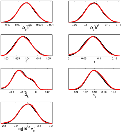
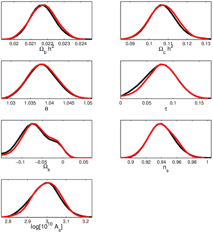
Figure 4: The one-dimensional marginalised posteriors on the cosmological parameters within the 7-parameter non-flat cosmology comparing: CAMB power-spectra and WMAP3, 2dF and SDSS likelihoods (red) with (a) CosmoNet power spectra and WMAP3, 2dF and SDSS likelihoods (black) and (b) CosmoNet likelihoods (black).

To determine the speed up introduced by using CosmoNet spectra and likelihood interpolations, 4 parallel MCMC chains were run on Intel Itanium 2 processors at the COSMOS cluster (SGI Altix 3700) at DAMTP, Cambridge using the basic CosmoMC sampling package. The time required to generate $\sim 20000$ post burn-in MCMC samples was recorded using methods (i)–(iv) described above . The results (see Table 2) illustrate that using CosmoNet spectra one can obtain reasonable posterior distributions in roughly 8 hours on a single CPU per chain whereas using CAMB not only took between 2-3 times longer but required 3 additional CPUs per chain. Using CosmoNets likelihood interpolations alone produced dramatic time savings, with accurate results in roughly 30 minutes.

Cosmologists have invested considerable time in developing samplers that have as efficient a proposal distribution as possible. In CosmoMC, the multi-variate Gaussian proposal distribution has a covariance matrix that is regularly updated using statistics from the samples gathered up to that point. This does lead to a higher acceptance rate and a corresponding lower number of likelihood evaluations, but is computationally intensive in its own right. However, when using a CosmoNet likelihoods directly there is no need to reduce the number of likelihood calls. The process of updating the proposal distribution slows the task considerably, as can be seen when comparing times with the efficient, yet likelihood intensive Bayesys sampler (Skilling, 2004) via method (iv), computing the relevent posteriors in just 3 minutes.

The reader should also note from both our previous work (Auld et al., 2007), and that of the 10 parameter models below, that the timings for parameter estimation are roughly independent of the number of model parameters used. Our regression algorithm is indifferent to the complexity of the input cosmology.

Method	(i)	(ii)	(iii)	(iv)
No. chains	4	4	4	4
No. CPU/chain	4	1	1	1
Run time	$>$ 16 hrs.	$\sim 8$ hrs.	$\sim 30$ mins.	$\sim 3$ mins.

Table 2: Time required to gather $\sim$ 20,000 post burn-in MCMC samples using different combinations of CAMB, CosmoNet, the experimental likelihood codes and Bayesys. Note that CAMB is parallelised in method (i) over 4 CPUs per chain, if a single processor were used these timings would approach 4 $\times$ that quoted.

5 Towards a 10 dimensional parameter space

In Auld et al. (2007) we presented trained networks capable of replacing CAMB and experimental likelihood codes for a 6 parameter flat cosmology. In this paper we have shown that this method is easily extendable to the more arduous computational demands of a non-flat cosmology. To test the scaleability to even higher dimensions we now examine a 10 dimensional cosmology including, in addition to the basic 7 given in Sec. 3: the equation of state of dark energy, $w$, the neutrino mass fraction, $\nu$ and the tensor to scalar ratio, $r$.

Training efficiency was examined as per the 7 parameter model (see Table 3) and it was found that little increase in the quantity of training data or training time was needed for optimum results for the CMB power spectra and matter transfer function. An accurate tracer of the scaling of the training algorithm is given by the number of network hidden nodes as this determines the amount of computational resource required. In this case we find that at worst a $50\%$ increase in the number of hidden nodes is needed for a $\sim 40\%$ rise in the number of parameter dimensions (going from 7 to 10). This represents slightly more than a linear rise in resources and demonstrates our algorithm is easily scaleable to even higher dimensions if necessary. The accuracy of interpolated CMB spectra and matter transfer functions did not decrease at all when compared to the 7 parameter interpolations (see Fig. 5), suggesting that the largest source of error in our method is introduced by fixing the set of $\ell$ and $k$ values at their flat positions. Providing an accurate interpolation for the three likelihood surfaces was however problematic. Using the order of 1000 training data provides very sparse coverage of the 10 dimensional hypercube. For CMB power spectra and the matter transfer function this is not a problem since they vary smoothly over a limited dynamical range. For likelihoods however, the dynamical range is much larger and to obtain parameter constraints we need very good accuracy within a region having a volume of the order of that of a $1\sigma$ hypersphere. This hypersphere has a volume over 400,000 times less than the 10 parameter $4\sigma$ hypercube over which we performed the training. This suggests that much more training data would be required. A potential solution to this problem would be to train likelihood networks only in some region over which the likelihood value was within (say) 50 log units of the peak value. The shape of this region could be determined by a classification net that returns an output that predicts whether a point lies inside or outside the desired region. This method will be explored in a future publication.

	Training Data	Hidden Nodes
CMB Spectra	2000	75
MPT Function	2000	50

Table 3: The required number of data, and hidden nodes in the neural network training for optimum performance in a 10 dimensional parameterisation.

\psfrag{xlabel}{\tiny$\ell$}\psfrag{ylabel}{\tiny Error in $C_{\ell}^{TT}$}\includegraphics[width=81.66545pt,angle={-90}]{PLOTS/L_2000/C_TT.eps}

\psfrag{xlabel}{\tiny$\ell$}\psfrag{ylabel}{\tiny Error in $C_{\ell}^{TE}$}\includegraphics[width=81.66545pt,angle={-90}]{PLOTS/L_2000/C_TE.eps}

\psfrag{xlabel}{\tiny$\ell$}\psfrag{ylabel}{\tiny Error in $C_{\ell}^{EE}$}\includegraphics[width=81.66545pt,angle={-90}]{PLOTS/L_2000/C_EE.eps}

\psfrag{xlabel}{\tiny$\ell$}\psfrag{ylabel}{\tiny Error in $C_{\ell}^{BB}$}\includegraphics[width=81.66545pt,angle={-90}]{PLOTS/C_bb.eps}

\psfrag{xlabel}{\tiny$\ell$}\psfrag{ylabel}{\tiny\% Error}\psfrag{xlabel}{\tiny k}\includegraphics[width=81.66545pt,angle={-90}]{PLOTS/C_MPT.eps}

Figure 5: Comparison of the performance of CosmoNet versus CAMB for TT, TE, EE and BB power spectra (a-d) and matter transfer function (d) in a 10 parameter non-flat cosmological model. The CMB plots show the average error together with the 95 and 99 percentiles in units of cosmic variance. The transfer function is shown with % error.

Marginalised posteriors obtained from CosmoNet spectra were found to be accurate to within a few $\%$ of those computed via CAMB (see Fig. 6), and took roughly 8 hours on a single CPUs per chain to calculate (see Table 4). CAMB however required more than 20 hours of computational time with parallelisation over a further 4 CPUs per chain.

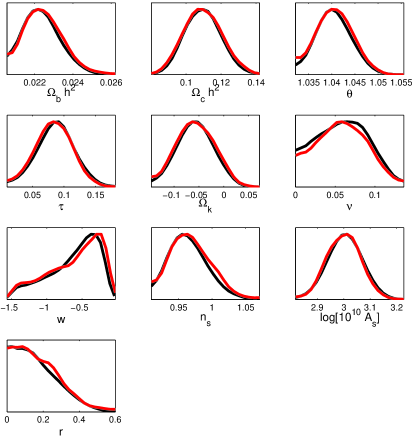
Figure 6: The one-dimensional marginalised posteriors on the cosmological parameters within the 10-parameter non-flat $\Lambda$CDM model including tensor modes, varying equation of state of dark energy and massive neutrinos comparing: CAMB power-spectra and WMAP3, 2dF and SDSS likelihoods (red) with CosmoNet power spectra and WMAP3, 2dF and SDSS likelihoods (black).

Method	(i)	(ii)
No. chains	4	4
No. CPU/chain	4	1
Run time	$>$ 20 hours	$\sim 8$ hours

Table 4: Time required to gather $\sim$ 20,000 post burn-in MCMC samples using different combinations of CAMB, CosmoNet and the experimental likelihood codes. Note that CAMB is parallelised in method (i) over 4 CPUs per chain, if a single processor were used these timings would approach 4 $\times$ that quoted.

6 Discussion and Conclusions

We have extended our method of accelerating the estimation of CMB and matter power transfer functions, WMAP, 2dF and SDSS likelihood evaluations based on training a multilayer perceptron neural network to more generic non-flat cosmologies. We have demonstrated that the use of trained neural networks such as CosmoNet can replace the bulk of computational effort required by cosmological evolution codes such as CAMB and experimental likelihood codes, like that of WMAP3. CosmoNet shares all the improvements made by Pico in terms of accuracy on both spectral interpolation and parameter constraints, but has now been scaled to a more generic 7 parameter non-flat cosmology. Furthermore, although the training procedure requires the optimisation of a highly non-linear multi-dimensional function, the end user simply runs the MemSys package essentially as a ‘black box’. This means CosmoNet remains simple and efficient to train. We have found the biggest bottleneck in the procedure to be the generation of training and testing data using CAMB. Increasing the model complexity had limited impact on the necessary training time (all models taking about 100 hours to train) or interpolation accuracy. Moreover the increase in network hidden nodes was at worst linear with increasing parameter space. Thus we expect few resource difficulties in extending this method to even higher dimensions.

Although accurate likelihood interpolations in the 10 dimensional model interpolation are currently beyond the reach of our method, the corresponding CMB spectra and matter transfer functions are sufficiently accurate allowing a speed up over the standard performance of CosmoMC.

Finally, replacing the CosmoMC sampler entirely with Bayesys can produce further dramatic time savings of a factor of $\sim 10$, computing $\sim 20,000$ post burn-in samples in a few minutes on a single CPU.

ACKNOWLEDGMENTS

TA acknowledges a studentship from EPSRC. MB was supported by a Benefactors’ Scholarship at St. John’s College, Cambridge and an Isaac Newton Studentship. This work was conducted in cooperation with SGI/Intel utilising the Altix 3700 supercomputer at DAMTP Cambridge supported by HEFCE and PPARC. We thank S. Rankin and V. Treviso for their assistance.

References

- Auld et al. (2007) Auld T., Bridges M., Hobson M. P., Gull S. F., 2007, MNRAS, 376, L11
- Bailer-Jones (2001) Bailer-Jones C., 2001, Automated Data Analysis in Astronomy. Narosa Publishing House, New Delhi
- Dickinson et al. (2004) Dickinson C., et al., 2004, MNRAS, 353, 732
- Fendt & Wandelt (2007) Fendt W. A., Wandelt B. D., 2007, ApJ, 654, 2
- Gull & Skilling (1999) Gull S., Skilling J., 1999, Quantified maximum entropy: MemSys 5 users’ manual. Maximum Entropy Data Consultants Ltd, Royston
- Habib et al. (2007) Habib S., Heitmann K., Higdon D., Nakhleh C., Williams B., 2007, ArXiv Astrophysics e-prints
- Hinshaw et al. (2006) Hinshaw G., et al., 2006, ArXiv Astrophysics e-prints
- Hobson & Lasenby (1998) Hobson M. P., Lasenby A. N., 1998, MNRAS, 298, 905
- Jimenez et al. (2004) Jimenez R., Verde L., Peiris H., Kosowsky A., 2004, Phys.Rev.D, 70, 023005
- Jones et al. (2006) Jones W. C., et al., 2006, ApJ, 647, 823
- Kaplinghat et al. (2002) Kaplinghat M., Knox L., Skordis C., 2002, ApJ, 578, 665
- Kosowsky et al. (2002) Kosowsky A., Milosavljevic M., Jimenez R., 2002, Phys.Rev.D, 66, 063007
- Kuo et al. (2004) Kuo C.-l., et al., 2004, Astrophys. J., 600, 32
- Lewis & Bridle (2002) Lewis A., Bridle S., 2002, Phys.Rev.D, 66, 103511
- Lewis et al. (2000) Lewis A., Challinor A., Lasenby A., 2000, ApJ, 538, 473
- Montroy et al. (2006) Montroy T. E., et al., 2006, ApJ, 647, 813
- Percival et al. (2001) Percival W. J., et al., 2001, MNRAS, 327, 1297
- Piacentini et al. (2006) Piacentini F., et al., 2006, ApJ, 647, 833
- Readhead et al. (2004) Readhead A. C. S., et al., 2004, Astrophys. J., 609, 498
- Rosenblatt (1958) Rosenblatt F., 1958, Psychological Review, 65, 386
- Sandvik et al. (2004) Sandvik H. B., Tegmark M., Wang X., Zaldarriaga M., 2004, Phys.Rev.D, 69, 063005
- Seljak & Zaldarriaga (1996) Seljak U., Zaldarriaga M., 1996, ApJ, 469, 437
- Skilling (2004) Skilling J., , 2004, BayeSys3 Users Manual
- Tegmark et al. (2004) Tegmark M., et al., 2004, Astrophys. J., 606, 702