Coronal Abundances in Orion Nebula Cluster Stars

Abstract

Following the Chandra  Orion Ultradeep Project (COUP) observation, we have studied the chemical composition of the hot plasma in a sample of 146 X-ray bright pre-main sequence stars in the Orion Nebula Cluster (ONC). We report measurements of individual element abundances for a subsample of 86 slightly-absorbed and bright X-ray sources, using low resolution X-ray spectra obtained from the Chandra ACIS instrument. The X-ray emission originates from a plasma with temperatures and elemental abundances very similar to those of active coronae in older stars. A clear pattern of abundances vs. First Ionization Potential (FIP) is evident if solar photospheric abundances are assumed as reference. The results are validated by extensive simulations. The observed abundance distributions are compatible with a single pattern of abundances for all stars, although a weak dependence on flare loop size may be present. The abundance of calcium is the only one which appears to vary substantially between stars, but this quantity is affected by relatively large uncertainties.

The ensemble properties of the X-ray bright COUP sources confirm that the iron in the emitting plasma is underabundant with respect to both the solar composition and to the average stellar photospheric values. Comparison of the present plasma abundances with those of the stellar photospheres and those of the gaseous component of the nebula, indicates a good agreement for all the other elements with available measurements, and in particular for the high-FIP elements (Ne, Ar, O, and S) and for the low-FIP element Si. We conclude that there is evidence of a significant chemical fractionation effect only for iron, which appears to be depleted by a factor 1.5–3 with respect to the stellar composition.

1. Introduction

Chemical composition is one of the key properties of astrophysical environments, fundamental for classifying stellar populations and studying the evolutionary history of galactic chemistry over different spatial scales. Several processes altering element abundances in the vicinity of individual stars are particularly efficient in the early phases of stellar evolution: selective trapping in grains, high-energy photon and particle irradiation of the circumstellar medium, mass exchange between stars and protoplanetary disks via accretion and outflows, and fractionation effects in stellar coronae and magnetospheres. In pre-main sequence systems, these physical processes occur on short time scales and cause dramatic changes as new planetary systems form out of the circumstellar nebula. One of the widely discussed issues is why planet-hosting stars appear to be characterized by a metallicity higher (by 0.24 dex, on average) than stars without planets (Santos et al., 2005, and references therein).

The Orion Nebula Cluster (ONC) is one of the best studied star forming regions in the sky, and the chemical composition of the associated H II region has been historically considered a standard reference for ionized gas in the nearby Galaxy (Esteban et al., 2004). Optical spectroscopy of the nebula is the traditional approach employed to study the abundances of important elements in this environment, as well as in other star forming regions, because of the difficulty in obtaining photospheric abundance measurements for faint, rapidly rotating young stars. Abundance studies of Orion stars have been performed mainly on B main-sequence members (Cunha & Lambert, 1992, 1994; Simón-Díaz et al., 2006; Cunha, Hubeny, & Lanz, 2006). Only a few measurements are available for slowly-rotating F and G stars (Cunha, Smith, & Lambert, 1998) and K-M members (Cunha & Smith, 2005).

An alternative way to determine the chemical composition of late-type stars is emerging from X-ray spectroscopy (Güdel, 2004, Favata & Micela 2003, and references therein). The ONC was selected in 2003 for a very long observation program in X-rays with the Chandra  satellite, known as the Chandra  Orion Ultradeep Project (COUP, Getman et al., 2005). This program is providing an unprecedented wealth of information about the stellar population of the ONC and various characteristics of this prototypical stellar and planetary nursery.

Among the salient global properties of the ONC, Feigelson et al. (2005) noted the presence of a strong spectral feature around 1 keV in the cumulative spectrum of all detected X-ray sources, identified with the emission line complex due to H-like and He-like Ne ions in hot plasma associated with $\sim 1400$ ONC members. The prominence of this feature suggests a high abundance of Ne in the X-ray emitting plasma, a characteristic already observed in other magnetically active stars (see review by Güdel, 2004) together with an apparent depletion of iron in corona with respect to the expected photospheric composition.

This behavior is linked to the First Ionization Potential (FIP) of the elements and possibly to the stellar activity level: the composition of the coronal plasma in the Sun, and particularly in long-lived magnetic structures, appears enriched by low-FIP elements ($FIP<10$ eV) by about a factor 4 with respect to photospheric values. This is known as the FIP effect (e.g. Feldman & Laming, 2000), a characteristic observed also in other low-activity stars (Favata & Micela, 2003, and references therein). High-activity RS CVn-type and Algol-type binaries stars exhibit a different behavior with a tendency for low-FIP elements such as iron to become depleted with respect to high-FIP elements like argon and neon. This is called “inverse FIP effect” (Brinkman et al., 2001).

The above scenario requires further investigations for several reasons. First, photospheric abundances are usually uncertain due to severe NLTE and rotational broadening effects on optical spectra of active stars, and solar values are often employed as the reference for the stellar coronal abundances. The solar photospheric composition itself has been recently questioned by Asplund (2005), based on detailed 3-D modeling of the solar atmosphere. Moreover, the photospheric Ne abundance is not directly measurable even in the Sun because no Ne lines occur at optical wavelengths.

Second, the driving mechanism(s) for FIP-related fractionation in stellar upper atmospheres still escapes a clear understanding although some models have emerged (Arge & Mullan, 1998; Schwadron, Fisk, & Zurbuchen, 1999; Laming, 2004).

Third, the situation is made more complex by the presence of very high Ne abundance ratios in two classical T Tauri stars (CTTS), TW Hya and BP Tau, where the soft X-ray emission is often attributed to an accretion shock rather than to magnetic activity (Kastner et al., 2002; Stelzer & Schmitt, 2004; Schmitt et al., 2005). An alternative explanation for these high Ne abundances has been suggested based on an origin of the plasma in gas accreted from the circumstellar disks where refractory elements may be depleted into solids undergoing growth into planetary bodies (Drake, Testa, &Hartmann(2005), 2005). However, X-ray variability characteristics strongly favors CTTS X-ray emission dominated by magnetic flares rather than accretion (Stassun et al., 2006; Stelzer et al., 2007).

The COUP observation provides us with the largest homogeneous sample ever studied to address the issue of element abundances in X-ray emitting plasmas associated to young stars. Here we can exploit ensemble statistical properties to overcome uncertainties in individual stellar measurements. The uncertainties on abundances derived from X-ray spectra, even those obtained with the highest spectral resolution, may be larger than formal statistical error bars (Schmitt & Ness, 2004; Maggio et al., 2005). The large COUP stellar sample can compensate for this difficulty.

To address these issues, we present in this paper the results of a detailed analysis of CCD-resolution X-ray spectra of ONC members to derive the abundances of individual elements for a large number of young stars. In §2, we introduce the observation and the sample selection, §3 is devoted to the methodology of analysis, while the results are presented in §4 and discussed in §§5–9.

2. Observation and sample selection

The COUP data were obtained in January 2003 with the Advanced CCD Imaging Spectrometer (ACIS; Garmire et al., 2003) on-board the Chandra  X-ray Observatory (Weisskopf et al., 2002) by combining six consecutive observations of the Orion Nebula Cluster (ONC) with the same aimpoint and roll angle. The resulting data set has a total exposure time of $\sim 838$ ks (9.7 days) distributed over 13.2 days. The data reduction and analysis resulted in 1616 detected X-ray sources, of which about 1408 are associated with ONC stars (Getman et al., 2005). X-ray spectra and light curves for each source were constructed from events collected in a polygonal region centered at the source position including $\sim 90\%$ of the encircled energy. Here we employ the spectra and the related auxiliary response files (ARFs), created with the acis_extract software, as explained in Getman et al.

The criteria for sample selection were motivated by the need to perform a detailed analysis of the ACIS spectra, and – more specifically – to determine both the plasma temperature distribution in the corona and the abundances of a number of individual elements. The main requirement for this kind of analysis is a very strong signal (noise is negligible in these cases) and an excellent knowledge of the instrument spectral response. We select stars with at least $5000$ total (net) counts in the 0.5-8 keV energy band. Sources heavily affected by pile-up (flagged “a” in Table 6 of Getman et al., 2005) are excluded but the sample includes 23 stars with “mild” pile-up effects (“w” flag) for which the usual whole extraction region was used. We exclude four early-type stars ($T_{\rm eff}>10,000$ K) as their X-ray emission likely originates in wind shocks rather than in a corona. However, we have retained 34 stars with unknown $T_{\rm eff}$. The final sample contains 146 COUP sources listed in Table 1; about half of them have more than $8000$ total counts, and $55$ exceed $10^{4}$ counts.

Further a posteriori selection was made based on the amount of interstellar absorption exhibited in the X-ray spectra. Reliable determination of the abundances of some elements is possible only for slightly absorbed sources. We will focus our attention on the 86 sources with intervening hydrogen column densities $N_{H}<6\times 10^{21}$ cm^-2.

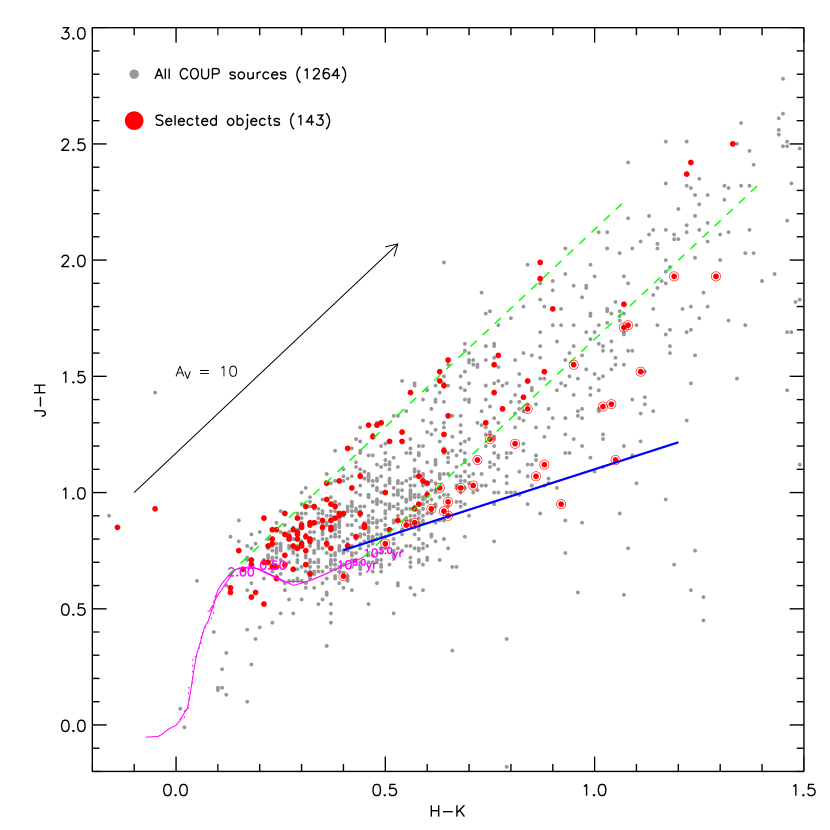
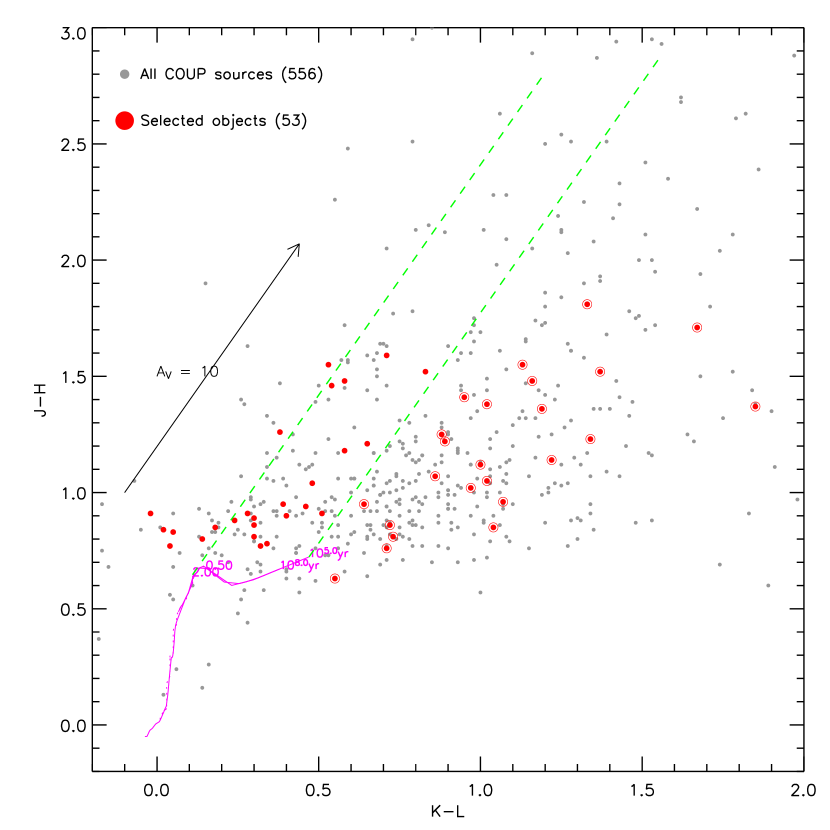
Figure 1.— Near-infrared color-color diagrams of the COUP sources with the stars in the present study indicated by filled red circles. The number of stars in the two diagrams differ because of incomplete IR photometric data for some of them. In magenta, the locus of stars with ages 1–5 Myr (Siess, Dufour, & Forestini, 2000, using $T_{\rm eff}$-color conversions by Kenyon & Hartmann, 1995). The black arrow indicates a reddening vector corresponding to $A_{\rm v}=10$, the dashed green lines bracket the region where stars with no NIR excess are expected, and the blue segment marks the locus of dereddened classical T Tauri stars (Meyer et al., 1997).

The optical properties of the 146 stars in our initial sample are reported in Table 1, based on the tables in Getman et al. (2005). Figure 1 shows two near-infrared (NIR) color-color diagrams for all the COUP detected sources with available photometric measurements in the NIR bands of interest. These diagrams show the theoretical locus of stars at the appropriate ONC age, and loci populated by objects with different amounts of reddening. Twelve sources fall to the right and below these loci in both color-color diagrams indicating they probably have dusty circumstellar disks in addition to reddening. Three of these sources plus two more without NIR photometric excesses (COUP 382, 579, 597, 758, and 1409) reveal protoplanetary disks seen in silhouette against the bright nebula (“proplyds”) in Hubble Space Telescope imaging (Kastner et al., 2005).

Table 1 also reports the equivalent width of the 8542 Å Ca II line from the study of Hillenbrand (1997). In 14 cases, this line is in emission with equivalent width larger than 1 Å, suggesting that the central star is actively accreting material from the circumstellar medium.

3. Analysis

Essentially all X-ray bright COUP sources show significant variability of their X-ray emission level (Getman et al., 2005; Favata et al., 2005; Wolk et al., 2005). In many cases, this variability is associated with large flares which are well-fit by a solar-type flare model where plasma is suddenly heated by a magnetic reconnection event and cools on timescales of hours-to-days (Favata et al., 2005). In the present work, we perform the X-ray spectral analysis collecting photons over the whole observation length which includes quiescent and flaring episodes. This may confuse interpretation of elemental abundances, as both temperatures, and sometimes FIP effects, vary during stellar flares (e.g. Audard, Güdel, & Mewe, 2001; Osten et al., 2004; Nordon, Behar, & Güdel, 2006). Our results thus give thermal and chemical characteristics of the emitting plasma which are spatially and temporally averaged over for each star. This conflation of ‘quiescent’ and flare conditions may not be avoidable as there may not exist any true ‘quiescent’ state in very active stars such as those in the ONC because, even during periods of little variability, the X-ray emission likely arises from a superposition of a multitude of weaker flares (Güdel, 2004 and references therein). This continuous flaring paradigm implies that the abundance properties we derive for the COUP sources probably describe time-averaged dynamical conditions rather than static equilibrium conditions of the X-ray emitting plasma.

We assume that the observed emission can be modeled as a collisionally-excited plasma in ionization equilibrium, and we adopt the emissivities predicted by the Astrophysical Plasma Emission Code (APEC V1.3.1, Smith et al., 2001) in the spectral fitting process. This choice, rather than the MEKAL emissivities (Mewe et al., 1995) adopted in previous COUP works, is motivated by the significantly larger number of emission lines and more updated atomic data of APEC vs. MEKAL as implemented in the XSPEC spectral analysis package. This is especially important in our work, aimed to derive information from line complexes due to specific atomic species of individual elements, which can be resolved at most only marginally in the available CCD spectra. In any case, this choice may affect the abundance measurements of some elements, but not our global results.

The data sets and instrument spectral response for each source are obtained from the data reduction described by Getman et al. (2005). Special features of the COUP data processing include a $0.5-8$ keV energy range and, for these strong sources, grouping of energy channels such that there are at least 60 net counts in each spectral bin.

3.1. Spectral diagnostics of element abundances

We adopt a global spectral fitting approach with multi-temperature models where individual element abundances are free parameters, in addition to the temperature and volume emission measure of each component and the interstellar hydrogen column density $N_{\rm H}$ to the star. Photoelectric absorption in the interstellar medium (ISM) is modeled with cross-sections obtained by Morrison & McCammon (1983). The spectral resolution of ACIS CCDs is such that a model with two or three isothermal components usually provides a good description of the observed spectra. This modeling approach provides an approximate description of the continuous distribution of temperatures undoubtedly present in the X-ray emitting plasma, but it is certainly adequate to the amount of information provided by instruments with resolution power $\approx 10$–30.

For the abundance measurements, we consider the elements O, Ne, Mg, Si, S, Ar, Ca, Fe, and Ni. At the coronal temperatures typical of young active stars ($T\approx 10^{7}$ K), all of these atoms have important H-like or He-like ion lines in the ACIS wavelength range (1.5–27.6 Å, Fig. 2). Iron and Nickel are also represented by a large number of L-shell emission lines. However, clear spectral signatures of each element depends on several factors: relative line emissivities, plasma emission measure $vs.$ temperature distribution, line blending, interstellar absorption and, of course, the abundance of each element in the plasma. Due to the complexity of these dependencies, we have performed extensive sets of simulations to validate our spectral fitting results. Details on these simulations are reported in Appendix and will be included in discussion of specific results below.

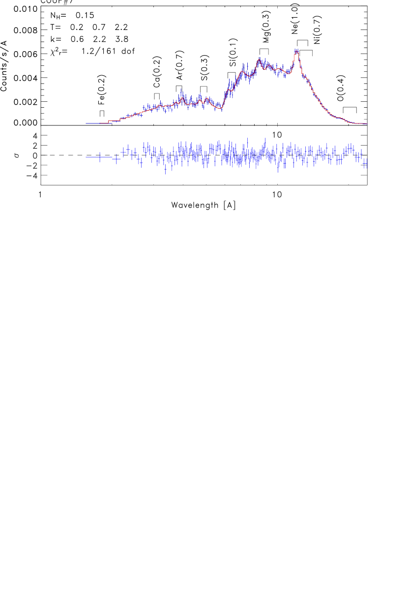
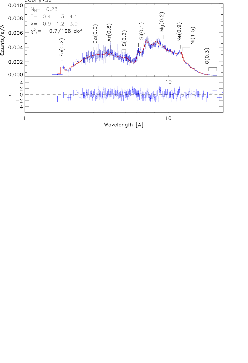
Figure 2.— Examples of spectra of Orion COUP sources with major emission line complexes labeled by their element abundances (in solar photospheric units). The best-fit 3-T model parameters ($N_{\rm H}$ in units of $10^{22}$ cm^-2, $T$ in keV, $k$ in cm^-5) and the reduced $\chi^{2}$ are indicated in the top panels, while bottom panels show the residuals in units of standard deviation.

The neon abundance is especially interesting for several reasons. First, this abundance cannot be determined in stellar photospheres because of the lack of suitable absorption lines in optical spectra, hence X-ray data provide the best opportunity to perform such a measurement. Second, neon has the highest First Ionization Potential (FIP = 21.56 eV) of any atoms except helium, hence its abundance with respect to iron (with a low FIP) provides crucial information about the stratification of elements with different FIPs in stellar atmospheres (§ 1). Third, H-like and He-like Ne ions produce prominent emission lines at energies around 1 keV where $Chandra$/ACIS sensitivity is highest. The correct determination of the Ne abundance is not free of difficulties due to the proximity of its most intense emission lines with L-shell iron and nickel lines. Figure 3 shows this with a plot of the integrated emissivity of Ne, Mg, Fe, and Ni lines in the wavelength range 9–14.5 Å, vs. plasma temperature for a solar mixture of chemical elements (Anders & Grevesse, 1989). Although the Fe emissivity exceeds that of Ne for solar abundances, when the Ne/Fe ratio is several times the solar ratio as found in many active stars (Drake et al., 2001; Güdel, 2004), the strength of the Ne lines in this spectral range becomes comparable to or greater than that of the iron lines. Thus, Ne abundances in active stellar coronae are sufficiently high to bring this element within the reach of global spectral analysis, as we will illustrate shortly.

Figure 3.— Total emissivity of emission lines from Ne, Mg, Fe, and Ni ions in the wavelength range 9–14.5Å, vs. temperature from the APEC plasma model assuming the solar element abundances of Anders & Grevesse (1989).

3.2. Spectral fitting procedure

Our procedure starts with fitting of 2-temperature (2-T) and 3-temperature (3-T) plasma models to all the source spectra using a $\chi^{2}$-minimization algorithm implemented in the XSPEC (V11.3) package (Arnaud, 1996). This step is repeated a few times with different starting values of the free parameters to avoid local minimum $\chi^{2}$ solutions. An F-test is then applied to determine whether the (usually lower) $\chi^{2}$ obtained with the 3-T model represent a significantly better fit to the data, or rather the improvement is entirely due to the larger number of free parameters with respect to the 2-T model. We adopt 3-T results only if the following two conditions are met: (i) the 2-T model has a poor fit with probability $P(\chi^{2})<10$%; and (ii) the F-test shows the 3-T model is significantly better with $P(F)<10\%$. The unnecessary introduction of a third thermal component, which typically has the lowest temperature, may alter the abundances of elements (such as O, Ne, and Mg) with emission lines only in the low-energy tail of the spectrum.

Our elemental abundances are scaled to the widely used solar system abundances of Anders & Grevesse (1989). In § 6 we will also discuss the implications of the recent solar composition recommended by Asplund et al. (2005).

This procedure resulted in 118 spectra fitted with a 2-T model and 28 spectra fitted with 3-T models. For 18 spectra, none of the models provides a statistically acceptable fit at the 99% confidence level, and in 12 of these cases the 3-T model is not significantly better than the 2-T model. This suggests that the poor fit is not due to the limited number of components adopted, but rather to other causes, perhaps residual problems in the calibration of the instrument response. Inspection reveals in most of these cases large residuals near the iridium edges at 5.7–5.9Å associated with the coating of the Chandra mirror. A formally better $\chi^{2}$ could be obtained by ignoring a narrow wavelength range in this spectral region, with little variations of the best-fit parameters. For several sources, we cannot exclude also an astrophysical process such as a departure of the plasma conditions from thermal equilibrium or temporal and/or spatial variations of element abundances in the emitting plasma. Recall that most of the sources are strongly variable and characterized by important flaring events. Nonetheless, since source variability is the norm rather than exception for ONC stars, we have not discarded any source based on a variability criterion.

3.3. Validation of spectral parameters

Figure 4.— Left: Comparison of absorption column densities obtained by Getman et al. (2005) with those in the present work. Right: Plot of absorption column density from COUP spectral fits vs. visual absorption. The two curves give the gas-to-dust relationship $N_{\rm H}=1.6\times 10^{21}A_{\rm v}$ (lower) and $N_{\rm H}=2.2\times 10^{21}A_{\rm v}$ (upper). Full symbols are used for stars in the count-limited sample.

We have estimated the uncertainty on individual quantities derived from these highly nonlinear spectral fits using the XSPEC code, with the criterion $\Delta\chi^{2}=2.7$ around $\chi^{2}$ minimum, corresponding to the 90% confidence level for one interesting model parameter at a time (Lampton et al., 1976). In particular, we have evaluated uncertainties in Fe and Ne abundances, elements with the strongest line signatures in our spectra, by allowing temperatures, emission measures, and abundances of the four elements with lines in the wavelength range 9–14.5 Å, (Ne, Mg, Fe, and Ni; see Figure 3) to vary freely. The resulting uncertainties are mostly less than a factor of two around the fitted value; more precisely, for half the measurements the relative error is within 30%, and it exceeds a factor 2 only in 5% of the cases (see error bars plotted in Figure 5).

We have evaluated the reliability of the derived abundances and their uncertainties in the simulations described in Appendix A. We find that the overall pattern of abundances for most elements is recovered with little bias by our analysis procedure, although some elements (Ca, Ni, Mg and O in particular) could be vulnerable to systematic errors. The XSPEC errors for Fe and Ne abundances are sometimes smaller than indicated by the simulations (§ 4.2).

One of the sources of uncertainty could be the actual emission measure distribution vs. temperature in the emitting plasma. To test the possibility that our element abundances derived from global spectral fitting could be affected by inadequate X-ray emission models, we have performed simulations with input emission measure distributions more complex than simple 2-T or 3-T approximations. We then checked that the plasma abundances are correctly recovered in spite of the mismatch between the actual source emission measure distribution and the adopted fitting model. For a few sample stars, we also fitted the observed X-ray spectra with alternative plasma emission models, having a fixed grid of temperatures and variable emission measures, and we have obtained abundance measurements consistent with the results presented above, within statistical uncertainties. These simulations and tests give us confidence that our spectral analysis provides us with a reasonably accurate description of the abundance patterns in the observed coronal plasma, at least for the sources without strong interstellar absorption (see below).

A final check on our spectral fitting is shown in Figure 4 where the derived interstellar hydrogen column densities ($N_{\rm H}$) are compared with values obtained by Getman et al. (2005) for all COUP sources and with dust reddening estimated from optical spectroscopy. Our values are very closely correlated to the COUP values except for a systemic offset by about 0.1 dex. We attribute this small discrepancy to the differences in the spectral fitting procedure used in the COUP analysis (1-T/2-T MEKAL plasma models rather than 2-T/3-T APEC models). The scatter in the $N_{\rm H}-A_{V}$ plot is similar to that seen in the full COUP sample.

Figure 5.— Scatter plots of best-fit abundance measurements of Fe (left) and Ne (right) vs. H column density. Plus and arrow symbols indicate upper limits. The heavy vertical line is drawn at the threshold value we have adopted to define our low-absorption sample.

As the $N_{\rm H}$ values in our sample exhibit a wide range from $\sim 2\times 10^{20}$ to $\sim 10^{23}$ cm^-2, we have investigated whether absorption might affect the elemental abundance measurements. Figure 5 shows a strong increase in the spread of Ne and Fe abundances, accompanied by larger statistical errors, as $N_{\rm H}$ increases. To minimize the influence of the above effects but still keeping the sample size as large as possible, we apply a threshold $N_{\rm H}<6\times 10^{21}$ cm^-2 (corresponding to $A_{\rm V}<3$–4) to avoid the high scatter in Ne and other abundances due to absorption. At this threshold, the attenuation at the Ne x Ly$\alpha$ wavelength (12.13 Å) is about a factor 4. There are 86 sources in our low-absorption sample, and we will focus our attention on them in the next sections.

4. Results

The best-fit spectral model parameters for the 86 stars in the low-absorption sample are reported in Table 2. A subset of 35 sources in this sample have more than $10^{4}$ counts in their spectra, and we will call it the count-limited subsample. The table gives the derived absorption, plasma temperatures and emission measures, abundances for 9 elements, the reduced $\chi^{2}$ of the fit, and the source X-ray flux in the 2–8 keV band. The median values of the abundance distributions and the central 68% ranges are reported in Table 3, for both the low-absorption sample and the count-limited subsample.

4.1. Coronal temperatures and elemental abundances

Figure 6 shows boxplots of temperatures, ratios of emission measures, and H column densities for the low-absorption subsample. These ONC stars are characterized by coronal plasma with temperatures ranging from $\approx 5$ MK to 25 MK (median values for the 2-T or 3-T models). The high-temperature components are dominant in most cases with emission measures typically two times larger than for the cool ($T<10$ MK) components. It is worth noting that the thermal characteristics of our sample stars are optimal for measuring Ne abundances, together with those of Mg and Ni, because the emissivities of the relevant emission lines peak in the same temperature range (see Figure 3).

Figure 6.— Box plots of temperatures, ratios of emission measures, and H column densities, derived from 2-T and 3-T fits (see Table 2). The upper and lower edges of each box comprise the central 68% of the data, the central value is the median. Squares mark individual measurements.

Figure 7.— Box plots of the best-fit abundance distributions for each element, sorted by increasing First Ionization Potential. The boxplot on the left in each pair refers to the full sample of slightly absorbed sources ($N_{\rm H}<6\times 10^{21}$ cm^-2), while the boxplot on the right pertains to the count-limited subsample ($>10,000$ extracted counts).

Boxplots of best-fit abundance values vs. First Ionization Potential (FIP) for the low-absorption sample and for the count-limited subsample are shown in Fig. 7. The three values indicated by each box (lower and upper edges, and central segment) represent the 68% range and the median reported in Table 3.

The striking feature of all these plots is the systematic pattern of abundance values vs. FIP: relatively low abundances with respect to the solar photospheric composition are consistently found for low-FIP elements Fe, Mg, and Si while elements with higher FIP are increasingly more abundant. Calcium and nickel abundances do not follow this trend, and our simulations (Appendix A) confirm the reliability of this result, in spite of some possible systematic error in the case of the Ca, and the sensitivity to line blending effects of the Ni measurement.

4.2. Reliability of the spectral analysis results

Before attempting any interpretation of the results we need to discuss their robustness against a number of possible sources of uncertainty. We first considered the count-limited subsample comprising the 35 sources with more than 10,000 counts, and the subsamples of sources with 2-T or 3-T best-fit models (74 and 12 sources, respectively). These yield essentially the same abundance distributions as the low-absorption sample, although with slightly different amount of scatter. Hence, the results do not depend on the source strength or assumed plasma temperature distribution.

We performed several simulations as described in Appendix A to investigate a variety of other possible effects. The simulations provide us with distributions of the best-fit abundances which take into account: the photon counting statistics at each wavelength, the possible cross-talk between elements with emission lines falling within the instrument spectral resolution, and the cross-talk between line strength and continuum level determined by the normalization of the thermal components. These simulations show that our procedures reliably recover true source coronal abundances. The observed FIP pattern is recognized self-consistently only in simulations with input models assuming that specific pattern, and FIP effects are not artificially introduced when they are not present.

Figure 8.— Cumulative distributions of Fe (left panel) and Ne (right panel) abundances: results from simulations employing 2-T models (dotted line) are compared with 2-T spectral fitting results for our count-limited subsample (heavy dashed line), and with the results for the full sample of slightly-absorbed sources (solid line). For both elements, the observed and simulated distributions are statistically undistinguishable at the 99% confidence level.

Uncertainties of the model abundances are evaluated through the simulations and found to have scatter similar to that seen in the observed sample. For 2-T or 3-T source model spectra and count rates typical of our COUP sources, our spectral analysis is able to recover the input values within a factor of 2 for Fe, Si, and S, and within a factor of 3 for Ni, O, Ar, and Ne. Mg and Ca abundances are the most uncertain by factors 5–10.

5. Coronal abundances in the X-ray luminous ONC stars

It is important to recognize that the sample of 86 ONC stars giving the results in Table 2 and Figure 7 is uniquely large and homogeneous in the field of stellar X-ray spectroscopy. Abundance measurements based on ACIS low-resolution CCD spectra are usually impractical due to either insufficient counts or pileup effects in high count rate stars. Abundance measurements based on high-resolution grating X-ray spectroscopy with Chandra and XMM-Newton are available up to now for less than 30 late-type stars with vastly different ages and in disparate astrophysical environments.

Given our large sample size, we can focus our attention on the subsample of 35 sources with more than 10,000 extracted counts which provides the most reliable abundance measurements. We have verified using Kolmogorov-Smirnov tests that the elemental abundance distributions for this subsample, are statistically indistinguishable from the distributions obtained for the sources having between 5000 and 10000 counts. However, our entire study is certainly biased toward the most magnetically active X-ray stars and is limited to slightly absorbed COUP sources. The characteristics of the more embedded Orion stellar population and of the stellar coronae with relatively lower X-ray luminosities are not treated here.

Figure 9.— Left: Cumulative distributions of the Ne/Fe abundance ratios for the full sample of slightly-absorbed sources (solid line) and for the count-limited subsample (heavy dashed line). Right: Scatter plot of Ne vs. Fe abundances, with error bars evaluated from individual spectral fits (§ 3.2), for the stars in the count-limited sample. The two straight lines indicate different Ne/Fe abundance ratios.

The next step is to establish whether our sample of 35 bright sources is consistent with a single distribution of coronal abundances without star-to-star variations. Figure 8 shows a comparison between the observed and simulated distributions of abundances for Fe and Ne. The simulation here was performed assuming a 2-T model with all parameters fixed at the median values of the observed distributions and taking into account the actual photon counting statistics of the observed spectra (Appendix A). A Kolmogorov-Smirnov test finds that the observed distributions are consistent with the simulations ($P\sim 10-20$%). Similar results are obtained for all the other elements, except for the peculiar case of the Ca (see below). Thus, the observed spread of abundances for each element is compatible with being due to the uncertainties on the measurements. There is no clear evidence for different coronal compositions among the ONC stars in the count-limited sample. However, we show below that marginally significant differences between certain subsamples may be present.

Inspection of Table 3 shows that the iron abundance of the coronal plasma in our full sample of X-ray bright ONC stars is well constrained in the range 0.12–0.37 times the solar value. The abundances of the low-FIP elements Mg and Si are compatible with the iron abundance, while the higher FIP elements S, O, Ar, and Ne appear systematically higher. Considering Fe and Ne as representative of the low-FIP and high-FIP species, respectively, we find a median Ne/Fe abundance ratio of 6$\pm$2 (Fig. 9 left). While the uncertainties on the measurements for individual stars can be large (Fig. 9 right), the median value is well-measured and the possibility that Ne/Fe=1 is confidently excluded.

Nickel and calcium abundances do not follow a simple FIP-abundance relationship. The relatively high abundance of the low-FIP Ni may appear suspicious. The atomic database we have employed contains a large number ($>1600$) of L-shell Ni lines in the range 5–24 Å, produced by all ions from Ne-like Ni XIX to Li-like Ni XXVI, which form at temperatures ranging from 8 MK to 25 MK, hence it is quite complete in this respect. The most prominent spectral lines are those of Ni XIX at 12.44, 12.66, 13.78, 14.04, and 14.08 Å, which fall close to the important H-like and He-like Ne lines, and a cross-talk between the two abundance parameters is possible. However, our simulations indicate that a high Ni abundance can be correctly recovered (Appendix A). We conclude that the high Ni abundance looks real, although the uncertainties may be larger than for other elements.

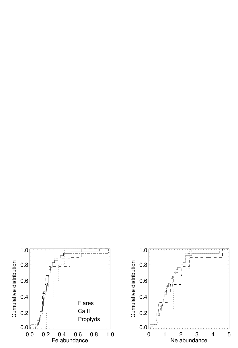
Figure 10.— Cumulative distributions of Fe (left panel) and Ne (right panel) abundances for the count-limited sample (solid line) and for three different stellar groups: X-ray sources associated with proplyds (dotted line), stars with Ca II in emission (heavy dashed line), and stars with evidence of large flares (dot-dashed line).

The best-fit calcium abundances are zero for about 70% of the stars in our sample, independently from the amount of hot plasma indicated by the best-fit model. But Ca K-shell lines are clearly visible at $\sim 3$ Å in the spectrum of several COUP sources and give high measured Ca abundance values (Table 2). Other important L-shell lines from Ca XVI– XVIII fall in the range 19–24Å, i.e. at the end of the inspected ACIS band; these lines are much weaker than the O VII– VIII lines occurring in the same spectral region, and hence they are not useful for the determination of the Ca abundance. Simulations performed with the Ca abundance set to zero predict a distribution of best-fit Ca values which is below the observed distribution, and simulations assuming a solar Ca abundance give a higher distribution (Appendix A). This suggests either an intrinsic spread in Ca abundance is present in the sample, or that some unknown systematic error in the analysis affects calcium abundance estimates. At present, we believe that the reported underabundance of Ca in most sources is a solid result.

6. Abundances as a function of other properties

The above analysis indicates that the stars in our sample, chosen to have very high X-ray luminosities ($L_{\rm x}$ in the range $10^{29.8}$–$10^{31}$ erg s^-1), share similar temperature distributions and chemical abundances. These similarities represent a major result of the work presented here and suggest that a single physical mechanism is operative in the sample.

We can nonetheless investigate whether interesting subsamples behave as the whole population of X-ray-bright ONC stars. Inspection of the optical characteristics of our ONC sample (Table 1) reveals that our sample includes nine stars with Ca II in emission suggesting active accretion (COUP 11, 66, 112, 141, 567, 579, 670, 801, and 1608), and five stars associated with imaged proplyds (COUP 382, 579, 597, 758, and 1409). Seventeen stars in our sample were studied by Favata et al. (2005) for the presence of large flares in their COUP light curves; six (COUP 43, 141, 669, 752, 848, 1608) showed evidence of very long ($L>5R_{*}$) flaring magnetic loops.

In Figure 10, we compare the Fe and Ne abundance distributions for our count-limited sample with abundances of these three groups. We find that the X-ray sources associated with proplyds show on average higher abundances with respect to the sources in the count-limited sample, while the strong-Ca II stars and the stars in the flaring group are indistinguishable from the full sample. However, even in the former case, the distributions for the stars in the subsample are not significantly different from those in the count-limited sample at 90% Kolmogorov-Smirnov confidence levels.

Figure 11.— Cumulative distributions of Fe (left panel) and Ne (right panel) abundances for the count-limited sample (solid line) and for two subgroups of the X-ray sources studied by Favata et al. (2005) for the presence of large flares: stars with evidence of very long magnetic structures (dashed line), and the complementary sample of stars with shorter flaring structures (dotted line).

The case of the stars caught during strong flares is particularly interesting because time-resolved analyses of large flaring events in active stars have indicated in many cases an apparent increase of the plasma metallicity at the onset of the flare with respect to the quiescent phase (Favata & Micela, 2003, and references therein). We thus might expect that the COUP stars whose X-ray emission is dominated by strong flares could have higher Fe and Ne abundances. We do not observe this effect in Figure 10, where the flaring stars are considered all together.

A more intriguing case is offered by Fig. 11, which compares the abundance distributions of the long-loop stars with those characterized by shorter flaring loops, as derived by Favata et al. (2005). While the abundances in the short-loop flaring plasma tend to be higher than the average, the long-loop objects show systematically lower abundance values (also for the other elements not shown in figure). Kolmogorov-Smirnov tests performed between these two distributions yield probabilities $P=9$% (1%) that the Fe (Ne) abundances are drawn from the same parent population. These low probabilities suggests that we are indeed observing different classes of X-ray sources in the two groups, characterized by different chemical evolutions or different origins of the flaring plasma. Since the statistical significance of this result is not very high, specific time-resolved analyses of individual flaring events are required to confirm it.

7. Comparison with older magnetically active stars

We return to the ensemble properties of the X-ray bright, count-limited sample of 35 ONC stars to compare with other active stars for which high-quality X-ray spectroscopy is available. Fig. 12 shows the abundances ordered by FIP derived for our COUP sources with four comparison stars: the classical T Tauri star TWA 5 in the TW Hya association (Argiroffi et al., 2005), the weak-line T Tauri star PZ Tel in the $\beta$ Pic association (Argiroffi et al., 2004), the ZAMS star AB Dor (Sanz-Forcada, Maggio, & Micela, 2003b), and the active binary system V851 Cen (Sanz-Forcada, Favata, & Micela, 2004). The abundances for these four stars were derived from high-resolution grating spectra taken with Chandra and/or XMM-Newton, and hence with techniques more refined than the global spectral fitting approach used here.

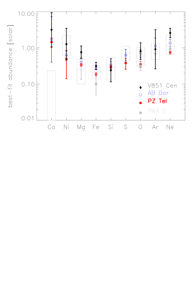
Figure 12.— Comparison of abundances derived for the COUP sources (box plots of the fitting results for the count-limited subsample) with the abundances obtained from the analysis of high-resolution grating spectra of four active stars: TWA5, PZ Tel, AB Dor, and V851 Cen.

The similarity of the abundance patterns $vs.$ FIP in the Orion and older stars is striking, except for the discrepant calcium abundances. The X-ray bright ONC stars share with other active stars a characteristic Ne/Fe abundance ratio several times the solar ratio (Drake et al., 2001; Güdel, 2004). This behaviour is often attributed to an underabundance of low-FIP elements with respect to high-FIP elements, i.e. to the so called ”inverse FIP effect” (Brinkman et al., 2001). Such a behaviour was recently observed also in young, weak-line T Tauri stars (Argiroffi et al., 2004, 2005), and now we find it in the X-ray bright ONC stars.

In recent years, the number of coronal sources with available abundance determinations has increased steadly, but we are far from a clear assessment of the phenomelogy. In fact, a variety of abundance patterns has been observed, with more or less pronounced deviations from both the classical solar FIP effect and the inverse FIP effect in its original version. For example, the four comparison stars in Fig. 12 show the inverse-FIP effect between iron and neon but they are all characterized by relatively high abundances for the low-FIP elements Ca, Ni, and Mg. Some star-to-star differences in the abundance patterns appear to be linked to the stellar activity level (Audard et al., 2003; Güdel, 2004; Garcia-Alvarez et al., 2006), but again with striking exceptions. Wood & Linsky (2006) have recently reported the case of the binary 70 Oph where the primary shows a prominent solar-like FIP effect while the secondary has no FIP bias or possibly a weak inverse FIP effect, in spite of the similarity between the two stars in all other respects.

8. Revised treatment of standard abundances

Part of the confusion is likely due to our ignorance of true stellar photospheric abundances of the magnetically active stars, which are usually assumed to be solar, or at least with the same ratios as in the solar photosphere. When proper stellar abundance measurements are employed, the abundance vs. FIP pattern is no longer very clear (Sanz-Forcada et al., 2004).

8.1. Orion photospheric and nebular abundances

In the case of the ONC, an assessment of the photospheric composition is available only for a handful of stars. The chemical evolution of the Orion association was studied by Cunha & Lambert (1992, 1994) who derived photospheric CNO, Si and Fe abundances for 18 main-sequence B stars. One of the results of these early works was that the spread in O and Si abundances was larger than expected based on the measurement uncertainties. This is thought to indicate a real spread among stars of different ages, caused by self-enrichment of the nebula as a consequence of supernova explosions within the Orion association. However, the result could also be affected by systematic errors in the analyses, due to approximations in the adopted NLTE model atmospheres and line-blanketing effects. In fact, detailed calculations of the oxygen abundances for 3 B stars in Orion recently presented by Simón-Díaz et al. (2006) yield values lower by $\approx 0.2$ dex with respect to those of Cunha & Lambert (1994) for the same stars.

Figure 13.— Comparison between the abundances derived for the COUP sources in the count-limited subsample – scaled by two different sets of reference solar values as indicated – with the abundances obtained for 11 B-type stars in the Trapezium (Cunha & Lambert, 1994; Cunha et al., 2006), 8 F-G stars (Cunha et al., 1998), and for the Orion nebula (Esteban et al., 2004).

Cunha et al. (2006) report NLTE Ne abundances for 11 B-type stellar members of Orion and found a homogeneous abundance of neon, $A({\rm Ne})=8.27\pm 0.05$, and oxygen, $A({\rm O})=8.70\pm 0.09$ (in a log scale where $A({\rm H})=12$). For the same sample, we have computed average Si and Fe abundances from the measurements of Cunha & Lambert (1994): $A({\rm Si})=7.16\pm 0.15$, and $A({\rm Fe})=7.46\pm 0.12$. These values will be used in the next section.

For later-type stars, Cunha et al. (1998) determined NLTE oxygen and LTE Fe abundances from optical spectroscopy of 9 pre-main-sequence F and G Orion stars. Cunha & Smith (2005) report a study of fluorine, C and O abundances in 3 Orion K-M dwarfs. These works indicate that the solar-type stars of the Orion association all have the same Fe abundance: $A({\rm Fe})=8.40\pm 0.15$. In contrast, the oxygen abundance appears to vary from star to star with a large spread ($A({\rm O})=8.94\pm 0.36$ for the full sample), and we will not consider these measurements in the following.

Finally, we consider the composition of the Orion Nebula, which is the brightest and nearest Galactic H II region in the sky. Esteban et al. (2004) present echelle spectrophotometry of a region S-W of $\theta^{1}$ Ori C and derive abundances of several ionic species, including Ne I and Ne II, from collisionally-excited lines or recombination lines. Their analysis takes into account spatial variations of the temperature structure of the nebula and, applying ionization and dust-depletion corrections, obtain abundances of several gas-phase elements.

8.2. Revised solar abundances

Asplund, Grevesse, & Sauval (2005) present a detailed 3-D hydrodynamic modeling of the solar atmosphere and find that the abundances of many elements (including C, N, O, Ar, Ne, and Fe) need to be revised downward by factors of 1.5–2.4 from the widely-used compilation of Anders & Grevesse (1989). But the new solar composition implies lower opacities and produces a severe inconsistency between the standard solar interior model and precise helioseismology measurements (Antia & Basu, 2005; Bahcall et al., 2005). One solution to this conundrum is to revise upward the poorly-known Ne abundance in the Sun, bringing it closer to the values often measured in stellar coronae. From high-resolution X-ray spectroscopy of several active late-type stars, Drake & Testa (2005) showed that the coronal Ne/O abundance ratio is, on average, a factor 2.7 times higher than the solar value recommended by Asplund et al. (2005). A similar result was obtained by Cunha et al. (2006), who presented measurements of the photospheric Ne abundance in a sample of B-type stars in Orion, and obtained a Ne/O abundance ratio a factor 2.5 higher than the most recent solar value.

We also find the COUP sources in the count-limited sample we have obtained a median Ne/O ratio of 0.33, i.e. a factor 2.2 higher than the Asplund, Grevesse, & Sauval (2005) value. However, this ratio suffers large scatter in individual objects (the central 68% of the data span the range 0.11–1.18), possibly because oxygen measurements are the most affected by uncertainties in the amount of absorption and in the amount of low-temperature plasma (see Appendix A).

8.3. ONC coronal abundances with revised standard abundances

The boxes in Fig. 13 shows our Orion coronal abundances inferred from the COUP X-ray spectra with respect to the traditional Anders & Grevesse (1989) and revised Asplund et al. (2005) solar abundances. We have not adjusted the solar neon abundance as suggested by the work of Drake & Testa (2005). The boxplot shows that the inverse-FIP abundance pattern for our ONC stars is still present, and is even slightly more pronounced, with the Asplund et al. (2005) solar abundances.

The points with error bars in Figure 13 show average stellar photospheric abundances and nebular abundances (not corrected for dust-locking effects) as described in § 8.1, scaled by the Asplund et al. (2005) revised solar abundances (a similar scaling is made by (Esteban et al., 2004)). Our COUP coronal abundances for the high-FIP elements S, O, Ar, and Ne are very similar to those of the nebula, and also show good agreement with the stellar photospheric values for Si, O, and Ne. Thus, while we do find a strong inverse FIP effect with respect to solar elemental abundances, the effect disappears when Orion photospheric and nebular abundances are considered.

However, discrepancies are found in the iron abundances which appear significantly lower in the X-ray coronal plasma than in the stellar photospheres. The very low Fe abundance found for the gaseous nebula can be attributed to heavy depletion into grains. If the value derived for the B-type and F-G stars is indeed representative of the iron abundance in the photospheres of all the late-type ONC stars, Figure 13 suggests that the coronae of these stars are depleted in iron by a factor 1.5–3.

9. Summary and conclusions

• The coronal temperatures and elemental abundance pattern in X-ray luminous ONC stars is remarkably similar to that found from the analysis of high-resolution grating spectra of older magnetically active stars. Hence accretion or the presence of circumstellar disks does not appear to affect the X-ray production mechanism or plasma. The abundance of calcium is a possible exception: it appears to be extremely low in about 70% of the ONC stars we have studied. However, it is difficult to reliably measure low calcium abundances with the available CCD spectra.

• Comparison of the observed abundance distributions among different stars with simulated distributions indicate that all stars may actually have the same abundance values, i.e. the abundance spread for each element is compatible with the statistical uncertainties. Nonetheless, our results also suggest possible systematic differences between the abundance distributions for selected subsamples (e.g. those of the sources with short $vs.$ long flaring magnetic structures), which require a specific time-resolved spectral analysis to be confirmed.

• The ensemble properties of the COUP X-ray brightest sources confirm the low metallicity of the coronal plasma with respect to the solar photospheric value: the median Fe abundance is $\approx 0.2$ times the Anders & Grevesse (1989) value, or $\approx 0.3$ times the most recent determination by Asplund et al. (2005). At the same time, the Ne/Fe abundance ratio is significantly higher than the solar one, with a median value $\approx$ 5–7, depending on the assumed set of solar abundances.

• The X-ray brightest COUP sources show a clear pattern of abundances vs. FIP. Extensive simulations make us confident about the robustness of this result. If the solar photospheric abundances are adopted for reference, the low FIP elements (Mg, Fe, and Si) appear to have similar low abundances, 0.2–0.3 times the solar values, while Ni and the high-FIP elements (S, O, Ar, and Ne) appear to have higher abundances, 1–2 times the solar ones. However, comparison with abundance measurements obtained by means of optical spectroscopy of members of the Orion association indicates a good agreement between photospheric and coronal abundances for Si, O, and Ne, while iron is significantly depleted in the X-ray emitting plasma with respect to the stellar photospheres, by about a factor of 3. We conclude that there is no clear FIP-related behaviour of the hot plasma abundances in the X-ray bright Orion stars, when proper stellar photospheric abundances are taken into account.

Appendix A Simulations to validate spectral modeling

We have performed several simulations, each with 1000 realizations, based on known 2-T, 3-T, or multi-temperature input models and different elemental abundance distributions. They are employed to assess realistic scatter of best-fit parameters, in particular on the abundances, and to test for bias in the fitted parameters. We have also performed specific simulations in which the photon counting statistics of the observed spectra is taken into account. The selected simulations are tailored for comparison with results based on our count-limited sample with more than $10^{4}$ total extracted counts. All simulations use the same ancillary response file (i.e. instrument effective area) and response matrix belonging to a real COUP source near the center of the ACIS field of view. The simulated spectra were rebinned as the actual data (§ 3) and the spectral fitting was performed on the same fixed energy range (0.5–8 keV) with the same XSPEC procedures. The background spectrum associated with the same source was used as a template in all the cases; it contributes $0.3$% of the total source+background counts and thus has negligible effect on the results. In all simulations, we assume hydrogen column density in the ISM photoelectric absorption model component of $N_{\rm H}=3\times 10^{21}$ cm^-2, which is near the median value found for the COUP sources in our low-absorption sample (§ 4.1).

The simulations described below are sorted by increasing complexity, so to explore different sources of uncertainty. For each simulation, we state the issue we have tested and we show the relevant results. These simulations validate both our ability to recover the correct abundance pattern from the analysis of ACIS spectra, and that the observed pattern does not arise in a spurious fashion by our analysis process.

The first simulation assumes a 3-T input model having temperatures, emission measures, and abundances set to values near the median of the distributions obtained for our sources in the low-absorption subsample. The three plasma components have $kT_{1}=0.4$ keV, $kT_{2}=0.8$ keV, and $kT_{3}=2.6$ keV ($\log T=$ 6.7, 7.0, and 7.5 K), and emission measure ratios $EM_{2}/EM_{1}=1.5$ and $EM_{3}/EM_{1}=3.5$. All simulated spectra here have 36,000 counts before applying Poisson noise, which is near the median value of the spectra which required 3-T best-fit models. Elemental abundances were fixed to the median values determined by fitting the sources in our count-limited sample; the Ca abundance, in particular, was set to zero.

Figure 14.— Box plots of the best-fit temperatures (left) and normalizations (right) derived by fitting 1000 simulated 3-T model spectra, each with 36,000 (within Poisson statistics). The upper and lower edges of each box comprise the central 68% of the data, the central value is the median. Diamonds mark the values in the input model.

Figure 14 shows the distributions of temperatures and volume emission measures derived by fitting the simulated spectra, while Fig. 15 shows the distributions of the abundances, sorted by First Ionization Potential (FIP) of the relevant elements. The boxplots indicate the range covered by the central 68% of the values. Since the simulation is based on a perfect alignment of the input and fitted spectral model, the scatter in parameter values serves as a reference for ”the best we can do” with Chandra/ACIS spectra.

Figure 15.— Box plots of the best-fit abundances derived by fitting 1000 simulated 3-T model spectra for sources with 36,000 and 16,000 counts to illustrate the effects of signal strength. Diamonds mark the values in the input model, and the meaning of the boxes is the same as in Fig. 14.

Figure 15 also shows the distributions of abundances derived from simulations of 3-T spectra with 16,000 counts, which is the median for all the sources in our count-limited sample. As expected, the width of the distributions is slightly larger for all elements than seen in simulations with 36,000 counts. Simulations based on 2-T rather than 3-T input spectral models and simulations using sources with the same distribution of counts as in our sample give results very similar to those in Figure 15; little additional spread in the derived abundance distributions is introduced by the different source model spectrum or by the photon counting statistics of the real COUP dataset.

Figure 16.— Box plots of the best-fit abundances derived by fitting 1000 simulated 2-T model spectra with different input abundance patterns: (left) 0.2$\times$ solar abundances; and (right) 1.0$\times$ solar abundances with low Fe abundance. Symbols and other details as in Fig. 14.

In all cases, we see very little bias in the derived spectral parameters; that is, the median values of the distributions lie close to (usually within $\pm$10% of) the input values. Temperature estimates become increasingly inaccurate for the lower temperature components ($\log T<7.0$ K, which also have associated emission measures lower than for the high-temperature component). Considering the results of all simulations, we find that Fe, Si and S abundances are generally accurate within 40–80% relative errors, while Ni, O, Ar and Ne have somewhat lower accuracy by factors 1.8–2.8; Mg shows the largest scatter, with uncertainties up to a factor 10 in simulations with 2-T models and low ($\approx 14,500$ counts) photon counting statistics; in the case of the Ca, whose input abundance was assumed to be zero, the statistical fluctuations make the best-fit result the most uncertain with any value between 0 and 0.8 acceptable.

For the cases of Fe and Ne, we have verified that the uncertainties indicated by the simulations are slightly larger (by factors 1.2–1.4, on average) than the XSPEC errors, computed at the 90% confidence level for single parameter. However, the results presented here show that the uncertainties on the best-fit abundances for all elements are sufficiently small to recover the input abundance pattern vs. FIP. For example, we ascertain that the Ne abundances exceed those of Fe with very high degree of confidence. The scatter on abundance ratios with iron is even lower than on individual abundances, because all abundance measurements are correlated with the iron one to a certain degree: in fact, the apparent abundance ratio Ne/Fe$\sim$6 is affected by $\approx 30$% uncertainty, according to our simulations.

Figure 16 explores the possibility that the interactions between parameters might create the observed FIP abundance effect as a form of systemic bias in the fitting procedure. Here we show the abundances emerging from 2-T input models assuming 0.2 solar abundances for all elements. No trend is evident in the reconstructed abundance pattern. A similar result is found for input models with 1.0 solar abundances, exhibiting less scatter due to the stronger emission lines. Note, in particular, that an high abundance of Ca could be correctly determined if it were present, but little could be inferred for the Ni abundance in this situation (quite different from the case of the COUP sources), due to the strong blends with lines from the other elements.

Figure 17.— Boxplots of temperatures, normalizations, H column densities, and abundances obtained by simulating 1000 spectra with an underlying V-shaped emission measure distribution vs. temperature, and fitted with 3-T models. In each panel, diamonds show the pattern of input parameter values.

Our final simulations test our ability to model more complex thermal distributions. Simple 2-T or 3-T models are only approximations to the actual thermal structuring of real coronae that must have continuous distributions of emission measure $vs.$ temperature. Schmitt & Ness (2004) warn that coronal abundances may be inaccurately estimated without continuous temperature distribution models, but this caveat applies to the analysis of high-resolution grating spectra. Fig. 17 shows a representative simulation in which we assumed a V-shaped emission measure distribution over the temperature range $\log T=6.0$–7.6 K, with a minimum around $\log T=6.5$ K, resembling distributions determined from high-resolution X-ray spectroscopy of very active stars (e.g., Sanz-Forcada, Brickhouse & Dupree 2003). The results of this simulation suggest that, although the 3-T model can not effectively recover the actual emission measure distribution, the input pattern of abundances can still be reliably measured. Note, in particular, that the inferred Ne is sometimes underestimated but is not significantly overestimated with respect to the input value. Distributions more skewed toward low values are those of the O and Mg abundances, but the median is always quite close to the input value.

Table 1Properties of sample stars

COUP		$M$	$\log t$	$A_{\rm v}$	$\Delta(I$-$K)$	EW(Ca)	$V$	$I$	$J$	$H$	$K_{\rm s}$	$L$
ID	Sp Type	($M_{\odot}$)	(yr)	(mag)	(mag)	(Å)	(mag)	(mag)	(mag)	(mag)	(mag)	(mag)
Low-absorption sample
7	K1-K4	2.12	5.55	0.75	-0.02	$\cdots$	11.38	9.89	8.85	8.10	7.95	$\cdots$
9	K0-K3	2.11	6.49	0.88	0.10	$\cdots$	12.39	11.12	10.22	9.65	9.46	$\cdots$
11	K1e-K7	0.69	5.74	0.42	1.37	-14.6	13.40	11.65	10.53	9.46	8.60	$\cdots$
23	K2	2.17	6.18	1.57	0.09	$\cdots$	12.72	11.11	10.01	9.33	9.09	$\cdots$
27	M0	0.53	6.23	0.94	0.42	1.8	15.77	13.61	12.16	11.37	11.05	$\cdots$
28	M0	0.53	6.01	0.63	0.30	1.6	14.95	12.91	11.53	10.84	10.53	$\cdots$
43	M1 (SB2)	0.40	5.85	1.36	0.50	1.4	15.57	13.06	11.23	10.38	10.08	$\cdots$
62	K2	1.52	6.84	3.06	1.28	0.0	15.75	13.56	11.23	10.21	9.53	$\cdots$
66	M3.5e	0.24	6.05	0.59	1.05	-2.8	17.22	14.28	12.13	11.20	10.63	$\cdots$
67	M2.5	0.29	4.52	1.13	0.32	0.0	15.46	12.64	10.85	9.97	9.62	$\cdots$
71	M1.5	0.37	6.10	0.03	0.26	1.6	15.29	13.21	11.88	11.19	11.01	$\cdots$
101	M4.5	0.16	5.68	0.35	0.15	2.9	18.19	14.93	13.09	12.45	12.05	$\cdots$
108	M1.5	0.37	6.09	0.21	0.71	1.5	15.41	13.26	11.66	10.82	10.54	$\cdots$
112	M2e	0.33	6.25	0.39	0.63	-0.7	16.39	14.01	12.49	11.64	11.29	$\cdots$
113	A7(?)	2.20	6.73	4.20	0.11	$\cdots$	13.55	11.73	10.32	9.65	9.37	$\cdots$
139	M2	0.33	6.20	0.18	0.71	0.9	16.03	13.73	12.12	11.28	10.91	$\cdots$
141	B9-A1	2.11	6.47	1.83	0.43	-17.8	12.94	11.36	10.23	9.42	8.99	$\cdots$
150	M2.5	0.29	5.00	1.51	0.44	1.5	16.38	13.41	11.48	10.61	10.29	$\cdots$
152	$\cdots$	$\cdots$	$\cdots$	$\cdots$	$\cdots$	$\cdots$	14.91	12.83	11.38	10.60	10.30	$\cdots$
173	M1.5	0.37	5.60	0.47	0.67	1.0	14.92	12.67	10.91	10.15	9.86	$\cdots$
177	K5	1.19	6.36	2.85	0.48	2.0	16.06	13.64	11.54	10.52	10.10	$\cdots$
188	K1-K2	2.16	6.25	2.21	0.23	$\cdots$	13.56	11.70	10.33	9.51	9.22	$\cdots$
202	M1.5-M4	0.37	5.62	0.47	0.38	1.5	14.98	12.73	11.24	10.44	10.12	$\cdots$
205	M2	0.33	6.13	0.34	0.64	1.2	15.94	13.58	12.08	11.19	10.90	$\cdots$
270	M1	0.41	5.98	0.24	0.32	1.5	14.93	12.86	11.45	10.68	10.38	10.34
328	K1-K6	1.72	6.48	0.85	0.08	1.8	13.20	11.78	10.76	10.05	9.87	$\cdots$
343	K4-M0	0.59	5.76	0.12	0.52	1.9	13.47	11.71	10.46	9.66	9.39	9.25
382	K2-M2	0.69	6.06	0.42	0.81	0.0	14.28	12.53	11.24	10.39	9.94	8.90
387	K0-M0	2.34	6.43	1.70	1.00	$\cdots$	12.69	11.16	9.70	8.83	8.26	$\cdots$
417	M1	0.41	6.24	0.37	$\cdots$	$\cdots$	15.82	13.70	12.12	11.30	11.04	$\cdots$
431	G0-K0	2.61	6.45	3.11	-0.01	$\cdots$	12.79	10.94	9.54	8.86	8.63	$\cdots$
459	M0.5	0.27	5.00	0.00	$\cdots$	$\cdots$	14.32	12.45	11.07	10.34	10.08	$\cdots$
470	K1-M0	0.52	5.95	0.81	1.08	1.5	15.00	12.89	10.72	9.91	9.60	8.87
567	F8-K5e	1.20	6.02	0.38	0.80	-3.5	12.94	11.48	10.18	9.26	8.62	$\cdots$
579	K2e-M4	0.33	5.16	0.00	1.31	-17.4	14.40	12.30	10.80	9.59	8.78	8.13
597	late-G	1.49	7.06	2.69	$\cdots$	4.5	14.44	12.69	11.47	10.61	10.06	9.34
600	M3.1	0.26	4.34	1.83	0.93	$\cdots$	16.30	13.04	11.13	10.18	9.26	9.66
648	K3-M1.5	0.72	5.30	2.29	$\cdots$	$\cdots$	14.58	12.10	10.44	9.53	9.14	9.16
669	K3-K4	1.52	6.30	1.96	0.36	$\cdots$	14.49	12.53	10.92	10.06	9.76	9.46
670	K4-M0	1.68	5.88	2.31	0.39	-1.0	13.96	11.86	10.27	9.31	8.66	7.59
672	$\cdots$	$\cdots$	$\cdots$	$\cdots$	$\cdots$	$\cdots$	14.59	12.18	10.65	9.80	9.43	9.25
718	K4-M1	0.55	4.65	1.25	0.43	$\cdots$	13.83	11.55	10.08	9.17	8.73	8.45
752	M0	0.54	6.32	0.07	0.62	1.1	15.07	13.25	11.79	11.02	10.74	$\cdots$
753	K6	0.91	6.29	0.87	0.28	1.8	14.57	12.79	11.63	10.77	10.32	$\cdots$
761	K2-K4	1.35	6.70	2.55	1.46	$\cdots$	15.83	13.64	11.13	10.06	9.48	8.62
801	K4-M0	0.70	5.59	1.47	0.80	-1.2	14.06	11.90	10.14	9.19	8.61	7.97
828	K2-K6	0.90	5.76	1.17	0.74	1.2	13.77	11.87	10.01	9.18	8.89	8.84
848	M2.5	0.29	6.07	1.72	0.50	0.0	17.52	14.47	12.43	11.67	11.30	10.59
867	K3-K7	2.62	5.56	2.76	-0.17	1.6	13.04	10.82	9.44	8.56	8.19	7.95
945	M1.5	0.37	5.83	0.55	0.23	0.0	15.35	13.07	11.61	10.83	10.60	$\cdots$
960	M3.5	0.24	5.56	2.72	-0.51	0.0	18.98	15.21	12.92	12.27	11.95	$\cdots$
971	K2.5-K7	0.69	5.77	0.00	$\cdots$	1.8	12.88	11.51	10.48	9.63	9.77	$\cdots$
982	K7	0.73	6.89	0.00	$\cdots$	1.8	$\cdots$	13.70	10.70	9.77	9.82	$\cdots$
997	$\cdots$	$\cdots$	$\cdots$	$\cdots$	$\cdots$	$\cdots$	15.63	13.42	11.63	10.68	10.31	9.92
1002	K2-K5	1.30	6.98	0.41	0.05	2.5	13.77	12.52	11.65	11.08	10.95	$\cdots$
1083	$<$M0	$\cdots$	$\cdots$	$\cdots$	$\cdots$	$\cdots$	15.15	12.96	11.12	10.08	9.72	9.24
1111	$\cdots$	$\cdots$	$\cdots$	$\cdots$	$\cdots$	$\cdots$	18.18	14.03	11.84	11.07	10.66	10.34
1127	K5.5-K7	0.90	6.05	3.69	-0.18	1.4	16.93	14.05	12.08	11.03	10.64	$\cdots$
1143	K1-K2	1.90	6.54	2.16	0.24	$\cdots$	14.17	12.33	10.76	9.95	9.68	9.38
1151	K6	0.91	5.76	1.05	0.28	1.9	13.61	11.76	10.48	9.64	9.40	$\cdots$
1246	M3.5	0.23	6.26	0.92	0.75	0.0	17.80	14.73	12.60	11.56	10.96	$\cdots$
1248	M0.5	0.47	5.93	1.16	0.58	1.7	15.47	13.14	11.44	10.50	10.19	$\cdots$
1252	M0	0.53	6.27	1.22	0.65	1.6	16.14	13.87	11.99	11.12	10.79	$\cdots$
1261	$\cdots$	$\cdots$	$\cdots$	$\cdots$	$\cdots$	$\cdots$	$\cdots$	13.20	12.41	11.63	11.27	10.93
1269	G8-K3	2.01	6.51	0.75	0.10	$\cdots$	12.34	11.12	10.13	9.54	9.41	$\cdots$
1311	K2-K4	1.53	6.23	1.80	0.06	$\cdots$	14.23	12.33	11.01	10.17	9.94	9.92
1350	G3-K3	2.20	6.60	1.15	0.12	1.7	11.78	10.59	9.70	9.15	8.97	$\cdots$
1355	M3.5	0.24	6.07	0.00	0.26	0.0	16.30	13.96	12.32	11.63	11.37	$\cdots$
1374	$\cdots$	$\cdots$	$\cdots$	$\cdots$	$\cdots$	$\cdots$	$\cdots$	15.22	12.75	11.76	11.16	$\cdots$
1384	K5-M0.5e	0.52	5.95	0.00	0.56	1.9	14.12	12.37	10.95	10.18	9.96	$\cdots$
1412	M1.5-M4	0.37	5.66	0.75	0.63	1.8	15.36	13.00	11.56	10.65	10.39	9.88
1424	M0-M1	0.53	6.06	1.07	0.62	1.2	15.51	13.30	11.53	10.67	10.35	$\cdots$
1429	M1	0.43	4.14	4.42	-1.41	1.2	17.20	13.50	12.00	11.11	10.90	10.60
1433	$\cdots$	$\cdots$	$\cdots$	$\cdots$	$\cdots$	$\cdots$	17.29	13.89	12.02	11.22	10.93	$\cdots$
1443	$\cdots$	$\cdots$	$\cdots$	$\cdots$	$\cdots$	$\cdots$	14.37	12.48	11.11	10.31	10.08	$\cdots$
1449	$\cdots$	$\cdots$	$\cdots$	$\cdots$	$\cdots$	$\cdots$	17.63	14.77	12.42	11.35	10.91	$\cdots$
1463	K8e-M1:	0.59	5.83	0.56	0.50	$\cdots$	14.12	12.19	10.78	10.00	9.50	$\cdots$
1487	M1 (SB2)	0.40	5.86	1.65	$\cdots$	$\cdots$	15.88	13.26	11.55	10.61	10.28	$\cdots$
1489	F9-K0	2.59	6.46	2.06	0.05	$\cdots$	11.72	10.30	9.31	8.61	8.40	$\cdots$
1492	M1.5	0.37	6.03	0.11	0.46	1.6	15.13	13.02	11.63	10.88	10.57	$\cdots$
1499	$\cdots$	$\cdots$	$\cdots$	$\cdots$	$\cdots$	$\cdots$	15.84	13.79	11.39	10.46	9.85	$\cdots$
1516	K1-K4	1.40	6.82	1.31	-0.20	1.8	14.37	12.77	11.72	11.05	10.89	$\cdots$
1521	K4	1.40	6.67	1.08	1.01	$\cdots$	14.31	12.69	11.24	10.36	9.83	$\cdots$
1568	K0-K1e	2.55	6.34	0.59	0.19	$\cdots$	11.30	10.20	9.36	8.84	8.63	$\cdots$
1595	M2.5	0.29	5.99	0.00	0.11	$\cdots$	15.57	13.25	11.89	11.19	10.97	$\cdots$
1608	M0.5e	0.48	6.23	0.93	1.41	-1.3	16.01	13.77	11.96	11.06	10.41	$\cdots$
High-absorption sample
90	M0	0.52	5.93	4.97	0.08	1.6	19.09	15.36	12.68	11.44	10.97	$\cdots$
115	K7	0.71	6.21	3.83	0.86	1.4	17.99	14.91	12.20	10.91	10.43	$\cdots$
131	K5	1.20	6.34	3.95	0.53	1.4	17.12	14.27	11.98	10.95	10.24	$\cdots$
183	G:	$\cdots$	$\cdots$	$\cdots$	$\cdots$	0.0	18.03	15.68	12.03	10.31	9.23	$\cdots$
223	K5	1.19	6.08	4.66	1.04	1.7	17.35	14.22	11.53	10.10	9.34	$\cdots$
262	K5	1.13	6.78	3.77	2.24	2.3	17.69	14.91	11.66	10.07	9.30	8.59
310	$\cdots$	$\cdots$	$\cdots$	$\cdots$	$\cdots$	8.9	17.91	14.65	11.76	10.40	9.62	$\cdots$
323	K6-M0	0.57	6.21	3.86	1.22	2.0	18.50	15.24	12.44	11.11	10.46	$\cdots$
331	$\cdots$	$\cdots$	$\cdots$	$\cdots$	$\cdots$	$\cdots$	$\cdots$	16.23	12.48	10.55	9.36	$\cdots$
342	$\cdots$	$\cdots$	$\cdots$	$\cdots$	$\cdots$	$\cdots$	$\cdots$	14.89	11.73	10.25	9.62	9.04
365	K4-K7	0.72	7.79	0.00	$\cdots$	0.0	$\cdots$	14.37	11.14	9.66	8.82	7.66
449	K7	$\cdots$	$\cdots$	$\cdots$	$\cdots$	0.0	17.00	15.38	12.26	10.45	9.38	8.05
452	K0-K3	2.02	6.17	5.36	0.61	1.4	17.04	13.86	11.03	9.73	8.99	$\cdots$
454	K2-K7	2.35	5.91	5.85	0.20	2.1	16.85	13.48	10.83	9.61	9.10	8.21
490	K6-K8	0.70	5.62	4.91	0.32	1.2	17.55	14.05	11.40	10.10	9.61	$\cdots$
499	K5-M1	0.69	5.92	2.65	0.06	1.2	16.19	13.57	11.68	10.71	10.35	$\cdots$
514	$\cdots$	$\cdots$	$\cdots$	$\cdots$	$\cdots$	$\cdots$	18.20	15.10	12.36	10.93	10.37	$\cdots$
554	$\cdots$	$\cdots$	$\cdots$	$\cdots$	$\cdots$	$\cdots$	$\cdots$	$\cdots$	12.50	12.72	10.42	8.25
561	K5	$\cdots$	$\cdots$	0.00	$\cdots$	1.0	$\cdots$	14.58	11.12	9.41	8.34	6.67
626	M1	0.41	6.02	3.47	0.62	0.7	18.30	14.97	12.38	11.19	10.78	$\cdots$
649	M0.5-M2.5	0.40	6.03	4.11	0.43	0.0	19.12	15.45	12.64	11.38	10.84	10.46
655	$\cdots$	$\cdots$	$\cdots$	$\cdots$	$\cdots$	$\cdots$	$\cdots$	$\cdots$	$\cdots$	13.40	10.38	7.70
682	K2-K5	1.86	6.05	2.56	$\cdots$	$\cdots$	14.26	12.12	10.78	9.26	8.63	7.26
697	K5-lateK	$\cdots$	$\cdots$	$\cdots$	$\cdots$	6.1	15.17	12.54	10.25	9.11	8.06	6.84
707	M2	0.33	5.38	1.21	0.83	1.6	16.04	13.34	11.41	10.36	9.77	8.75
720	$\cdots$	$\cdots$	$\cdots$	$\cdots$	$\cdots$	$\cdots$	$\cdots$	16.57	12.72	10.93	10.03	$\cdots$
758	G5-K0e	3.00	6.12	3.78	1.50	-12.3	13.79	11.45	8.78	7.76	7.13	6.16
766	$\cdots$	$\cdots$	$\cdots$	$\cdots$	$\cdots$	$\cdots$	$\cdots$	11.00	9.74	8.37	7.35	5.50
784	M1.5-M2e	$\cdots$	$\cdots$	0.00	$\cdots$	$\cdots$	$\cdots$	17.99	12.20	11.20	10.70	8.63
874	$\cdots$	$\cdots$	$\cdots$	$\cdots$	$\cdots$	$\cdots$	$\cdots$	$\cdots$	$\cdots$	14.31	12.46	10.36
894	$\cdots$	$\cdots$	$\cdots$	$\cdots$	$\cdots$	$\cdots$	$\cdots$	$\cdots$	13.81	11.82	10.95	$\cdots$
915	$\cdots$	$\cdots$	$\cdots$	$\cdots$	$\cdots$	$\cdots$	$\cdots$	$\cdots$	13.63	11.21	9.98	$\cdots$
939	$\cdots$	$\cdots$	$\cdots$	$\cdots$	$\cdots$	$\cdots$	18.67	14.93	11.49	9.97	8.86	$\cdots$
942	M0	0.52	5.90	5.04	$\cdots$	0.0	19.06	15.30	11.98	10.43	9.67	9.14
985	F8-K0	2.97	6.17	2.06	1.19	$\cdots$	12.23	10.56	8.69	7.75	7.37	6.91
1028	K2	1.60	6.78	2.72	1.45	$\cdots$	15.26	13.20	10.93	9.75	9.11	8.53
1035	$\cdots$	$\cdots$	$\cdots$	$\cdots$	$\cdots$	$\cdots$	$\cdots$	$\cdots$	13.62	11.25	10.03	$\cdots$
1040	$\cdots$	$\cdots$	$\cdots$	$\cdots$	$\cdots$	$\cdots$	$\cdots$	$\cdots$	13.99	11.49	10.16	$\cdots$
1071	K7-M0	0.69	5.92	1.57	1.29	1.6	15.09	12.89	10.38	9.26	8.38	7.38
1080	earlyKe-M0	1.98	5.25	7.77	1.41	-16.9	17.82	13.48	9.65	7.72	6.43	$\cdots$
1114	K0-K5:	$\cdots$	$\cdots$	$\cdots$	$\cdots$	-1.5	15.72	12.46	9.80	8.58	8.04	$\cdots$
1140	$\cdots$	$\cdots$	$\cdots$	$\cdots$	$\cdots$	$\cdots$	19.59	15.89	12.80	11.28	10.40	9.57
1158	M1:	0.41	6.08	2.65	$\cdots$	0.0	17.67	14.66	11.90	10.54	9.70	8.51
1161	M0	0.54	6.43	0.00	1.12	1.5	15.21	13.44	11.80	10.90	10.51	10.11
1304	$\cdots$	$\cdots$	$\cdots$	$\cdots$	$\cdots$	$\cdots$	$\cdots$	$\cdots$	$\cdots$	$\cdots$	$\cdots$	$\cdots$
1309	K1-K4	1.90	6.44	4.33	$\cdots$	$\cdots$	16.37	13.64	10.64	9.39	8.75	7.87
1335	K8e	0.64	6.64	1.10	2.18	-2.5	16.32	14.18	11.97	10.74	9.99	8.65
1341	$\cdots$	$\cdots$	$\cdots$	$\cdots$	$\cdots$	$\cdots$	$\cdots$	14.42	11.42	9.96	9.32	8.78
1343	$\cdots$	$\cdots$	$\cdots$	$\cdots$	$\cdots$	$\cdots$	17.65	14.63	12.02	10.61	9.78	8.83
1354	G0-M3	2.34	6.55	1.70	0.18	$\cdots$	11.97	10.61	9.67	9.04	8.80	8.25
1380	K4	1.52	6.27	3.78	0.87	$\cdots$	16.28	13.61	11.69	10.31	9.27	8.25
1382	M0	0.52	5.88	1.97	1.25	0.0	15.94	13.38	11.31	10.17	9.45	$\cdots$
1391	M1	0.41	6.03	3.80	1.53	1.4	18.69	15.23	12.14	10.57	9.92	$\cdots$
1409	K6-K8e	0.74	7.10	0.00	3.01	-6.3	15.36	13.98	11.70	10.15	9.20	8.07
1410	M1	0.36	7.56	0.57	2.30	0.0	18.54	16.34	13.60	12.31	11.85	$\cdots$
1421	M0	0.54	6.13	1.04	1.10	0.9	15.63	13.43	11.60	10.71	10.33	$\cdots$
1444	K8e	0.60	6.19	1.10	0.73	-4.1	15.55	13.41	11.78	10.94	10.43	$\cdots$
1456	$\cdots$	$\cdots$	$\cdots$	$\cdots$	$\cdots$	$\cdots$	$\cdots$	16.83	13.36	11.44	10.57	$\cdots$
1462	K1	2.54	6.25	3.09	0.18	$\cdots$	13.95	11.82	10.12	9.25	8.92	$\cdots$
1466	K3-K5	1.40	6.65	1.96	0.42	1.4	15.15	13.19	11.69	10.78	10.38	$\cdots$

Table 2Spectral analysis results

COUP	$N_{\rm H}$	$T_{1}$	$T_{2}$	$T_{3}$	$k_{1}$	$k_{2}$	$k_{3}$	Abundances (solar units)											$f_{\rm x}$
ID	(a)	keV	keV	keV	(b)	(b)	(b)	O	Ne	Mg	Si	S	Ar	Ca	Fe	Ni	$\chi^{2}_{\rm r}$	DoF	(c)
7	1.5	0.2	0.7	2.2	0.6	2.2	3.8	0.4	1.0	0.3	0.2	0.3	0.7	0.2	0.2	0.7	1.2	162	1.5
9	2.6	$\cdots$	0.8	3.1	$\cdots$	1.6	2.8	0.9	0.6	0.4	0.4	0.6	1.3	0.0	0.3	1.7	1.3	125	1.7
11	3.9	$\cdots$	0.6	5.4	$\cdots$	0.9	0.7	0.1	0.3	0.2	0.7	2.9	2.5	0.0	0.1	0.7	1.6	61	0.6
23	2.4	0.1	0.8	2.4	0.8	3.6	5.6	0.8	0.9	0.2	0.1	0.5	0.6	0.1	0.2	0.7	1.2	203	2.6
27	1.7	$\cdots$	0.7	2.7	$\cdots$	0.3	0.5	0.7	1.4	0.2	0.2	0.6	1.3	0.0	0.2	0.4	0.9	61	0.3
28	1.5	$\cdots$	0.6	3.4	$\cdots$	0.5	2.5	0.6	1.1	0.2	0.3	0.9	0.5	0.0	0.2	0.7	1.2	154	1.6
43	5.3	$\cdots$	0.3	2.6	$\cdots$	18.6	1.0	0.0	0.0	0.0	0.1	0.6	0.0	0.0	0.0	1.6	1.1	74	0.4
62	2.6	$\cdots$	0.6	3.1	$\cdots$	1.0	0.9	0.4	0.2	0.1	0.2	1.0	1.6	0.0	0.0	1.8	1.2	97	0.5
66	1.7	$\cdots$	0.7	3.2	$\cdots$	0.2	0.6	1.2	1.3	0.0	0.0	1.5	0.6	0.0	0.1	0.6	1.2	64	0.4
67	2.0	$\cdots$	0.7	2.4	$\cdots$	0.4	0.7	0.9	1.1	0.5	0.2	0.3	1.4	0.0	0.3	0.8	1.0	75	0.3
71	0.0	$\cdots$	0.7	2.9	$\cdots$	0.6	0.4	0.3	0.1	0.0	0.0	0.9	0.9	1.8	0.1	1.3	1.0	62	0.2
101	1.6	$\cdots$	0.9	3.7	$\cdots$	0.4	1.3	0.9	0.3	0.3	0.0	0.8	1.4	1.4	0.1	2.8	0.8	103	0.9
108	3.1	$\cdots$	0.4	2.9	$\cdots$	0.2	1.0	0.7	2.1	0.9	0.5	0.0	0.6	0.1	0.3	2.9	0.9	69	0.6
112	3.2	$\cdots$	0.6	2.5	$\cdots$	0.2	0.7	1.2	2.1	0.4	0.5	0.6	0.9	0.9	0.6	1.6	1.1	77	0.4
113	2.9	$\cdots$	0.8	2.3	$\cdots$	1.1	2.0	1.1	0.9	0.1	0.1	0.8	0.6	0.0	0.2	1.3	1.3	71	0.9
139	1.6	$\cdots$	0.8	2.7	$\cdots$	0.6	0.4	0.5	0.2	0.0	0.0	0.4	1.5	0.0	0.1	0.0	0.9	62	0.2
141	1.8	$\cdots$	0.8	4.0	$\cdots$	1.0	1.0	0.8	0.5	0.1	0.2	1.0	1.1	0.0	0.2	0.1	1.1	117	0.8
150	2.8	$\cdots$	0.7	2.8	$\cdots$	0.3	0.6	0.9	1.1	0.2	0.2	0.9	1.7	0.3	0.2	1.1	1.3	64	0.3
152	0.5	$\cdots$	0.7	2.7	$\cdots$	0.3	0.4	0.7	0.4	0.0	0.1	0.6	0.0	1.7	0.1	1.5	1.2	58	0.2
173	1.9	$\cdots$	0.8	2.7	$\cdots$	1.0	0.8	1.0	0.1	0.0	0.1	0.7	0.9	0.3	0.2	0.2	1.0	99	0.5
177	4.6	$\cdots$	0.8	3.1	$\cdots$	1.2	0.4	0.0	0.0	0.1	0.1	0.3	1.1	0.1	0.1	0.1	0.8	48	0.3
188	2.7	$\cdots$	0.7	2.5	$\cdots$	1.8	3.4	0.6	0.9	0.1	0.1	0.4	0.5	0.0	0.1	1.1	1.3	158	1.5
202	2.4	$\cdots$	0.5	2.2	$\cdots$	0.3	0.6	0.3	0.7	0.0	0.2	0.4	0.9	0.0	0.1	2.1	1.3	49	0.2
205	1.9	$\cdots$	0.8	4.0	$\cdots$	1.1	0.5	0.3	0.2	0.0	0.1	1.0	2.7	0.8	0.1	0.0	1.2	66	0.4
270	1.3	$\cdots$	0.8	2.3	$\cdots$	0.3	0.4	1.4	0.8	0.2	0.4	0.6	0.8	0.5	0.3	0.0	1.2	63	0.2
328	1.5	$\cdots$	0.6	2.0	$\cdots$	1.2	1.0	0.5	0.8	0.2	0.1	0.4	0.5	0.0	0.1	1.7	1.2	97	0.4
343	1.6	$\cdots$	0.7	3.1	$\cdots$	1.1	2.8	1.2	1.7	0.1	0.3	1.2	0.8	0.4	0.2	0.1	1.6	177	1.8
382	2.7	$\cdots$	0.6	2.3	$\cdots$	0.2	0.3	1.9	2.3	0.7	1.0	1.7	0.2	4.9	0.4	3.9	0.9	50	0.2
387	2.4	$\cdots$	0.7	2.5	$\cdots$	0.9	2.1	0.5	1.1	0.2	0.2	0.7	0.4	0.3	0.2	1.0	1.2	135	1.0
417	1.9	$\cdots$	0.8	3.0	$\cdots$	0.5	0.6	0.5	0.7	0.3	0.1	1.1	1.2	1.4	0.1	1.2	0.8	62	0.4
431	5.1	$\cdots$	0.9	2.4	$\cdots$	1.0	2.7	0.9	1.4	0.3	0.4	0.6	0.6	0.8	0.3	2.8	1.1	141	1.3
459	0.2	$\cdots$	0.7	2.7	$\cdots$	0.1	0.6	0.7	2.4	0.8	0.7	0.4	1.6	0.0	0.4	1.9	0.9	78	0.3
470	1.4	$\cdots$	0.8	2.7	$\cdots$	0.5	0.9	1.5	0.6	0.2	0.2	1.1	1.1	0.0	0.4	2.2	1.3	99	0.5
567	2.1	$\cdots$	0.7	3.0	$\cdots$	0.5	1.0	0.7	1.3	0.5	0.4	0.8	1.4	0.5	0.2	1.5	1.0	99	0.6
579	4.5	$\cdots$	0.4	4.4	$\cdots$	0.1	1.0	0.1	2.5	0.0	1.1	1.6	3.8	0.0	0.2	0.0	1.6	79	0.7
597	0.0	$\cdots$	0.7	2.4	$\cdots$	0.2	0.4	1.0	1.6	0.0	0.5	1.1	1.7	5.7	0.2	3.3	1.0	78	0.3
600	2.7	$\cdots$	0.6	2.4	$\cdots$	0.2	0.4	0.8	1.6	0.8	0.9	1.7	0.3	0.0	0.3	3.1	0.9	52	0.2
648	3.8	$\cdots$	0.6	2.7	$\cdots$	0.7	2.8	1.0	2.3	0.4	0.5	1.2	0.9	0.0	0.2	1.7	1.8	159	1.6
669	3.6	$\cdots$	0.6	3.0	$\cdots$	0.5	2.4	1.0	2.3	0.5	0.5	0.8	0.9	0.0	0.3	0.6	1.2	149	1.4
670	4.4	0.5	2.2	7.7	1.0	2.9	1.0	0.6	2.0	0.6	0.6	1.0	1.7	0.0	0.2	1.2	1.6	185	2.3
672	2.6	$\cdots$	0.4	2.5	$\cdots$	0.5	1.2	0.3	1.4	0.7	0.8	1.3	0.5	0.0	0.2	1.0	1.5	80	0.6
718	3.8	$\cdots$	0.6	2.9	$\cdots$	0.7	2.5	0.0	1.2	0.2	0.3	0.8	0.0	0.0	0.2	1.8	1.2	143	1.2
752	2.8	0.4	1.3	4.2	1.0	1.2	3.8	0.3	0.9	0.2	0.1	0.3	0.8	0.0	0.2	1.5	0.7	199	2.8
753	5.3	$\cdots$	0.4	2.1	$\cdots$	0.7	1.0	0.5	0.9	0.5	0.3	0.5	1.0	0.0	0.2	0.0	1.0	63	0.4
761	5.5	$\cdots$	0.8	2.8	$\cdots$	0.3	0.8	7.3	2.1	0.5	0.3	0.8	1.0	0.6	0.9	1.2	1.1	108	0.7
801	5.9	$\cdots$	0.4	3.6	$\cdots$	0.6	3.6	4.8	4.6	1.5	1.3	2.0	2.9	0.0	0.5	2.4	1.3	127	3.4
828	3.5	$\cdots$	0.5	4.0	$\cdots$	0.3	4.2	0.3	4.4	0.4	1.2	1.6	1.4	0.0	0.4	1.4	1.1	123	3.2
848	2.7	0.5	1.7	10.8	0.3	0.6	0.3	0.5	0.7	0.0	0.3	0.9	1.3	0.0	0.1	1.2	1.2	77	0.5
867	4.1	$\cdots$	0.6	2.7	$\cdots$	0.4	1.9	0.3	2.3	0.6	0.7	0.6	0.5	0.0	0.4	3.7	1.2	128	1.0
945	1.0	$\cdots$	0.4	1.9	$\cdots$	0.3	0.5	0.4	1.4	0.7	0.4	0.9	0.0	3.0	0.2	1.3	0.9	63	0.2
960	1.1	$\cdots$	0.7	3.3	$\cdots$	0.0	0.4	1.4	2.3	0.4	0.4	1.2	2.5	0.0	1.0	3.2	1.2	56	0.3
971	0.3	0.2	0.8	2.6	0.2	1.2	3.6	0.6	1.6	0.0	0.4	0.5	0.9	0.0	0.2	1.9	1.3	142	1.8
982	2.7	$\cdots$	1.3	4.7	$\cdots$	1.2	1.2	0.0	1.4	0.0	0.5	0.7	0.4	3.2	0.0	0.3	1.1	63	1.1
997	3.6	$\cdots$	0.7	3.0	$\cdots$	0.7	2.0	0.0	1.0	0.3	0.3	1.3	0.2	0.0	0.1	1.5	1.0	130	1.1
1002	0.6	$\cdots$	0.4	1.9	$\cdots$	0.9	0.7	0.2	0.8	0.1	0.2	0.5	0.1	0.3	0.1	1.3	0.9	76	0.2
1083	5.0	$\cdots$	0.6	2.6	$\cdots$	0.7	2.1	0.3	1.5	0.1	0.2	0.7	0.8	0.0	0.2	1.8	1.2	124	1.0
1111	3.8	$\cdots$	0.6	2.8	$\cdots$	0.2	0.8	2.6	2.4	0.7	0.5	1.0	0.7	0.0	0.4	2.1	1.3	81	0.5
1127	5.4	$\cdots$	0.5	2.0	$\cdots$	0.4	1.1	0.0	1.3	0.4	0.5	0.5	1.5	0.0	0.1	0.1	1.2	60	0.4
1143	1.8	$\cdots$	0.4	2.2	$\cdots$	0.4	1.7	0.3	1.8	0.5	0.4	0.6	1.0	0.0	0.1	1.2	1.2	119	0.7
1151	1.6	$\cdots$	0.7	2.6	$\cdots$	1.5	2.1	0.5	0.8	0.0	0.1	0.9	0.9	0.0	0.1	1.3	1.4	146	1.0
1246	4.3	$\cdots$	0.4	3.4	$\cdots$	0.3	1.0	1.3	1.8	0.2	0.5	0.1	0.3	0.0	0.3	1.3	1.2	85	0.6
1248	3.0	$\cdots$	0.8	2.5	$\cdots$	0.8	1.8	0.0	0.7	0.1	0.2	0.7	0.7	0.0	0.1	1.7	1.1	117	0.8
1252	4.7	$\cdots$	0.7	3.3	$\cdots$	0.3	0.6	1.4	1.5	0.6	0.6	1.1	0.6	0.1	0.5	1.7	1.1	59	0.4
1261	2.8	$\cdots$	0.6	3.5	$\cdots$	0.1	0.5	2.2	1.9	0.5	0.6	1.2	0.0	0.0	0.4	2.7	1.4	57	0.4
1269	1.5	0.4	0.8	1.8	1.1	1.4	2.7	0.4	1.1	0.4	0.1	0.3	0.6	0.0	0.2	0.3	1.1	136	0.9
1311	2.1	$\cdots$	0.5	2.2	$\cdots$	0.2	0.4	0.5	2.0	0.4	0.7	1.4	0.7	1.6	0.3	3.2	1.0	51	0.2
1350	2.2	0.5	0.9	2.3	1.0	1.2	2.8	0.6	0.8	0.3	0.3	0.6	0.5	0.1	0.2	1.2	1.4	145	1.3
1355	1.5	$\cdots$	0.4	2.0	$\cdots$	0.5	0.6	0.4	0.8	0.1	0.3	0.4	0.0	0.0	0.1	1.1	1.2	58	0.2
1374	4.2	$\cdots$	0.4	2.6	$\cdots$	0.1	0.9	0.0	2.1	0.3	0.2	0.8	0.7	1.0	0.2	1.3	1.3	56	0.4
1384	1.0	$\cdots$	0.4	3.2	$\cdots$	0.2	2.4	0.7	2.7	0.1	0.6	0.4	0.5	0.8	0.2	2.3	1.1	160	1.5
1412	1.6	$\cdots$	0.8	2.2	$\cdots$	0.3	0.6	0.7	0.7	0.4	0.3	1.1	0.3	1.8	0.3	1.2	1.0	74	0.3
1424	3.1	$\cdots$	0.5	2.1	$\cdots$	0.4	0.9	0.3	1.5	0.2	0.2	0.4	0.2	0.0	0.1	2.2	1.1	74	0.3
1429	1.1	$\cdots$	0.4	2.0	$\cdots$	0.2	0.6	0.3	2.0	0.0	0.3	0.4	0.1	0.0	0.2	0.6	1.1	52	0.2
1433	4.2	$\cdots$	0.4	2.5	$\cdots$	0.2	0.6	3.7	4.1	0.0	0.3	0.4	0.2	0.0	0.5	5.0	0.9	71	0.4
1443	2.2	$\cdots$	0.7	3.4	$\cdots$	0.2	0.8	1.7	2.0	0.4	0.8	1.3	0.0	0.4	0.5	2.3	1.2	97	0.6
1449	4.0	$\cdots$	0.4	3.3	$\cdots$	0.0	0.8	0.0	4.4	0.3	1.0	1.5	0.8	0.0	0.4	4.7	1.2	61	0.5
1463	0.7	$\cdots$	0.4	2.5	$\cdots$	0.2	0.8	0.4	1.7	0.2	0.4	0.4	0.2	0.0	0.3	1.9	1.1	79	0.3
1487	4.2	$\cdots$	0.4	2.2	$\cdots$	0.3	0.6	1.0	2.2	0.8	0.7	0.8	0.8	0.7	0.4	4.6	1.2	60	0.3
1489	1.9	0.4	0.8	2.0	0.4	0.5	1.5	0.4	1.2	0.5	0.4	0.7	0.3	0.3	0.2	1.2	1.4	107	0.5
1492	1.3	$\cdots$	0.7	2.4	$\cdots$	0.2	0.5	1.2	2.1	0.7	0.6	0.9	0.1	0.0	0.3	2.4	1.0	67	0.2
1499	5.9	$\cdots$	0.6	4.0	$\cdots$	0.2	0.7	4.0	2.1	0.8	0.9	2.1	1.6	1.4	0.6	0.0	1.0	65	0.7
1516	0.3	0.2	0.6	1.9	0.2	0.2	0.6	0.3	1.5	0.3	0.4	0.2	1.7	0.0	0.2	1.0	1.4	68	0.2
1521	1.5	$\cdots$	0.5	2.6	$\cdots$	0.4	1.0	0.1	1.7	0.5	0.4	0.7	0.0	0.0	0.1	0.2	1.6	93	0.5
1568	0.6	0.8	1.5	8.1	1.9	4.1	4.2	0.8	0.6	0.2	0.4	0.5	0.7	0.7	0.3	1.2	2.7	265	5.4
1595	0.3	$\cdots$	0.7	2.4	$\cdots$	0.5	0.3	0.7	0.8	0.2	0.3	1.0	0.0	4.2	0.1	1.6	1.8	60	0.2
1608	2.9	0.2	1.3	5.2	1.2	1.3	0.6	0.1	0.6	0.0	0.2	0.1	1.3	0.0	0.2	0.0	1.2	92	0.6

Table 3Abundances in ONC X-ray bright stars

		Low-absorption sample			Count-limited sample
	FIP	median	68% range		median	68% range
Element	(eV)	(Anders & Grevesse (1989) solar abundance units)
Ca	6.11	0.00	0.00	0.90	0.00	0.00	0.54
Ni	7.64	1.32	0.31	2.51	1.37	0.65	2.20
Mg	7.65	0.25	0.03	0.58	0.26	0.09	0.49
Fe	7.90	0.22	0.12	0.37	0.22	0.14	0.33
Si	8.15	0.33	0.14	0.70	0.30	0.13	0.55
S	10.36	0.75	0.43	1.23	0.74	0.45	1.13
O	13.62	0.57	0.25	1.26	0.60	0.29	1.00
Ar	15.76	0.76	0.20	1.52	0.76	0.49	1.33
Ne	21.56	1.34	0.59	2.23	1.14	0.65	2.27

References

- Anders & Grevesse (1989) Anders, E., & Grevesse, N. 1989, Geochimica et Cosmochimica Acta, 53, 197
- Antia & Basu (2005) Antia, H. M., & Basu, S. 2005, ApJ, 620, L129
- Arge & Mullan (1998) Arge, C. N., & Mullan, D. J. 1998, Sol. Phys., 182, 293
- Argiroffi et al. (2004) Argiroffi, C., Drake, J. J., Maggio, A., Peres, G., Sciortino, S., & Harnden, F. R. 2004, ApJ, 609, 925
- Argiroffi et al. (2005) Argiroffi, C., Maggio, A., Peres, G., Stelzer, B., & Neuhäuser, R. 2005, A&A, 439, 1149
- Arnaud (1996) Arnaud, K. A. 1996, in ASP Conf. Ser. 101, Data Analysis Software and Systems V, ed. G. H. Jacoby & J. Barnes (San Francisco: ASP), 17
- Asplund (2005) Asplund, M. 2005, ARA&A, 43, 481
- Asplund et al. (2005) Asplund, M., Grevesse, N., Sauval, A. J. 2005, in ASP Conf. Ser. 336, Cosmic Abundances as Records of Stellar Evolution and Nucleosynthesis, ed. T. G. Barnes III and F. N. Bash, 25
- Audard et al. (2001) Audard, M., Güdel, M., Mewe, R. 2001, A&A, 365, L318
- Audard et al. (2003) Audard, M., Güdel, M., Sres, A., Raassen, A. J. J., & Mewe, R. 2003, A&A, 398, 1137
- Bahcall et al. (2005) Bahcall, J. N., Basu, S., Serenelli, A. M. 2005, ApJ631, 1281
- Brinkman et al. (2001) Brinkman, A. C. et al. 2001, A&A, 365, L324
- Cunha et al. (2006) Cunha, K., Hubeny, I., & Lanz, T. 2006, ApJ, 647, L143
- Cunha & Lambert (1992) Cunha, K., & Lambert, D. L. 1992, ApJ, 399, 586
- Cunha & Lambert (1994) Cunha, K., & Lambert, D. L. 1994, ApJ, 426, 170
- Cunha & Smith (2005) Cunha, K., & Smith, V. V. 2005, ApJ, 626, 425
- Cunha et al. (1998) Cunha, K., Smith, V. V., & Lambert, D. L. 1998, ApJ, 493, 195
- Drake et al. (2001) Drake, J. J., Brickhouse, N. S., Kashyap, V., Laming, J. M., Huenemoerder, D. P., Smith, R., Wargelin, B. J. 2001, ApJ, 548, 81
- Drake & Testa (2005) Drake, J. J., Testa, P. 2005, Nature, 436, 525
- Drake et al. (2005) Drake, J. J., Testa, P., Hartmann, L. 2005, ApJ, 627, 149
- Esteban et al. (2004) Esteban, C., Peimbert, M., García-Rojas, J., Ruiz, M. T., Peimbert, A., Rodríguez, M. 2004, MNRAS, 355, 229
- Favata et al. (2005) Favata, F., Flaccomio, E., Reale, F., Micela, G., Sciortino, S., Shang, H., Stassun, K. G., Feigelson, E. D. 2005, ApJ, 160, 469
- Favata & Micela (2003) Favata, F., & Micela, G. 2003, SSRv, 108, 577
- Feigelson et al. (2005) Feigelson, E. D., Getman, K., Townsley, L., Garmire, G., Preibisch, T., Grosso, N., Montmerle, T., Muench, A., McCaughrean, M. 2005, ApJS, 160, 379
- Feldman & Laming (2000) Feldman, U., & Laming, J. M. 2000, Phys. Scr, 61, 222
- Garcia-Alvarez et al. (2006) García-Alvarez, D., Drake, J. J., Ball, B., Lin, L., Kashyap, V. L. 2006, ApJ, 638, 1028
- Garmire et al. (2003) Garmire, G. P., Bautz, M. W., Ford, P. G., Nousek, J. A., Ricker, G. R., Jr. 2003, SPIE, 4851, 28
- Getman et al. (2005) Getman, K. V., Feigelson, E. D., Grosso, N., McCaughrean, M. J., Micela, G., Broos, P., Garmire, G., & Townsley, L. 2005, ApJS, 160, 319
- Güdel (2004) Güdel, M. 2004, A&A Rev., 12, 71
- Hillenbrand (1997) Hillenbrand, L. A. 1997, AJ, 113, 1733
- Kastner et al. (2002) Kastner, J. H., Huenemoerder, D. P., Schulz, N. S., Canizares,
- Kastner et al. (2005) Kastner, J. H., Franz, G., Grosso, N., Bally, J., McCaughrean, M. J., Getman, K., Feigelson, E. D., Schulz, N. S. 2005, ApJS, 160, 511 C. R., Weintraub, D. A. 2002, ApJ, 567, 434
- Laming (2004) Laming, J. M. 2004, ApJ, 614, 1063
- Lampton et al. (1976) Lampton, M., Margon, B., & Bowyer, S. 1976, ApJ, 208, 177
- Kenyon & Hartmann (1995) Kenyon, S. J., Hartmann, L. 1995, ApJS, 101, 117
- Maggio et al. (2005) Maggio, A., Drake, J. J., Favata, F., Güdel, M. 2005, in ESA SP 560, Proceedings of the 13th Cambridge Workshop on Cool Stars, Stellar Systems and the Sun, ed. F. Favata, G.A.J. Hussain, B. Battrick, 129
- Mewe et al. (1995) Mewe, R., Kaastra, J. S., Liedahl, D. A. 1995, Legacy, 6, 16
- Meyer et al. (1997) Meyer, M. R., Calvet, N., & Hillenbrand, L. A. 1997, AJ, 114, 288
- Morrison & McCammon (1983) Morrison, R., McCammon, D. 1983, ApJ, 270, 119
- Nordon et al. (2006) Nordon, R., Behar, E., Güdel, M. 2006, A&A, 446, 621
- Osten et al. (2004) Osten, Rachel A.,g Brown, Alexander; Ayres, Thomas R.; Drake, Stephen A.,g Franciosini, Elena; Pallavicini, Roberto; Tagliaferri, Gianpiero,g Stewart, Ron T.; Skinner, Stephen L.; Linsky, Jeffrey L. 2004, ApJS, 153, 317
- Sanz-Forcada et al. (2004) Sanz-Forcada, J., Favata, F., & Micela, G. 2004, A&A, 416, 281
- Santos et al. (2005) Santos, N. C., Israelian, G., Mayor, M., Bento, J. P., Almeida, P. C., Sousa, S. G., Ecuvillon, A. 2005, A&A, 437, 1127
- Sanz Forcada et al. (2003a) Sanz Forcada, J., Brickhouse, N. S., & Dupree, A. K. 2003, ApJS, 145, 147
- Sanz-Forcada et al. (2003b) Sanz-Forcada, J., Maggio, A., & Micela, G. 2003, A&A, 408, 1087
- Schmitt & Ness (2004) Schmitt, J. H. M. M., & Ness, J.-U. 2004, A&A, 415, 1099
- Schmitt et al. (2005) Schmitt, J. H. M. M., Robrade, J., Ness, J.-U., Favata, F., Stelzer, B. 2005, A&A, 432, 35
- Siess et al. (2000) Siess, L., Dufour, E., & Forestini, M. 2000, A&A, 358, 593
- Simón-Díaz et al. (2006) Simón-Díaz, S., Herrero, A., Esteban, C., Najarro, F. 2006, A&A, 448, 351
- Smith et al. (2001) Smith, R. K., Brickhouse, N. S., Liedahl, D. A., & Raymond, J. C. 2001, ApJ, 556, 91
- Stassun et al. (2006) Stassun K. G., van den Berg, M., Feigelson, E., Flaccomio, E. 2006, ApJ, 649, 914
- Stelzer & Schmitt (2004) Stelzer, B., Schmitt, J. H. M. M. (2004), A&A, 418, 687
- Stelzer et al. (2007) Stelzer, B., Flaccomio, E., Briggs, K., Micela, G., Scelsi, L., Audard, M., Pillitteri, I., Güdel, M. 2007, A&A, in press
- Schwadron et al. (1999) Schwadron, N. A., Fisk, L. A., & Zurbuchen, T. H. 1999, ApJ, 521, 859
- Weisskopf et al. (2002) Weisskopf, M. C., Brinkman, B., Canizares, C., Garmire, G., Murray, S., Van Speybroeck, L. P. 2002, PASP, 114, 1
- Wolk et al. (2005) Wolk, S. J., Harnden, F. R., Jr., Flaccomio, E., Micela, G., Favata, F., Shang, H., Feigelson, E. D. 2005, ApJS, 160, 423
- Wood & Linsky (2006) Wood, B. E., Linsky, J. L. 2006, ApJ, 643, 444