A 3D radiative transfer framework: II. line transfer problems

Abstract

Context. Higher resolution telescopes as well as 3D numerical simulations will require the development of detailed 3D radiative transfer calculations. Building upon our previous work we extend our method to include both continuum and line transfer.

Aims. We present a general method to calculate radiative transfer including scattering in the continuum as well as in lines in 3D static atmospheres.

Methods. The scattering problem for line transfer is solved via means of an operator splitting (OS) technique. The formal solution is based on a long-characteristics method. The approximate $\Lambda$ operator is constructed considering nearest neighbors exactly. The code is parallelized over both wavelength and solid angle using the MPI library.

Results. We present the results of several test cases with different values of the thermalization parameter and two choices for the temperature structure. The results are directly compared to 1D spherical tests. With our current grid setup the interior resolution is much lower in 3D than in 1D, nevertheless the 3D results agree very well with the well-tested 1D calculations. We show that with relatively simple parallelization that the code scales to very large number of processors which is mandatory for practical applications.

Conclusions. Advances in modern computers will make realistic 3D radiative transfer calculations possible in the near future. Our current code scales to very large numbers of processors, but requires larger memory per processor at high spatial resolution.

1 Introduction

Hydrodynamical calculations in two and three spatial dimensions are necessary in a broad range of astrophysical contexts. With modern parallel supercomputers, they are also becoming more realistic, in that they can be run at modest to high resolution. Performing full radiation hydrodynamical calculations is presently still too computationally expensive. Recently, Hubeny & Burrows (2006) have presented a mixed frame method of solving the time-dependent radiative transfer problem in 2D, but their work is tailored toward neutrino transport where the absence of rapidly changing opacity such as a spectral line makes their approximations appropriate. Similar work has been presented by Mihalas & Klein (1982), Lowrie et al. (1999), and Lowrie & Morel (2001). Taking a different approach Krumholz et al. (2006) derive the flux-limiter to $O(v/c)$ for use in radiation hydrodynamics calculations. Similar work was presented by Cooperstein & Baron (1992). Even though these recent first steps are improvements, they suffer from a loss of accuracy, either in dealing with spectral lines, or in obtaining the correct angular dependence of the photon distribution function or the specific intensity. While these recent works are expedient, they are crude enough that the results of the hydrodynamical calculations cannot be compared directly with observed spectra. Given the fact that computational resources are finite, a final post-processing step is necessary to compare the results of hydrodynamical calculations to observations.

In Hauschildt & Baron (2006, hereafter: Paper I) we described a framework for the solution of the radiative transfer equation for scattering continua in 3D (when we say 3D we mean three spatial dimensions, plus three momentum dimensions) for the time independent, static case. Here we extend our method to include transfer in lines including the case that the line is scattering dominated. Fabiani Bendicho et al. (1997) presented a multi-level, multi-grid, multi-dimensional radiative transfer scheme, using a lower triangular ALO and solving the scattering problem via a Gauss-Seidel method. van Noort, Hubeny, & Lanz (2002) presented a method of solving the full NLTE radiative transfer problem using the short characteristics method in 2-D for Cartesian, spherical, and cylindrical geometry. They also used the technique of accelerated lambda iteration (ALI) (Olson et al. 1987; Olson & Kunasz 1987), however they restricted themselves to the case of a diagonal accelerated lambda operator (ALO).

We describe our method, its rate of convergence, and present comparisons to our well-tested 1-D calculations.

2 Method

In the following discussion we use notation of Hauschildt (1992) and Paper I. The basic framework and the methods used for the formal solution and the solution of the scattering problem via operator splitting are discussed in detail in paper I and will thus not be repeated here. We have extended the framework to solve line transfer problems with a background continuum. The basic approach is similar to that of Hauschildt (1993). In the simple case of a 2-level atom with background continuum we consider here as a test case, we use a wavelength grid that covers the profile of the line including the surrounding continuum. We then use the wavelength dependent mean intensities $J_{\lambda}$ and approximate $\Lambda$ operators ${\Lambda^{*}}$ to compute the profile integrated line mean intensities ${\bar{J}}$ and $\bar{\Lambda^{*}}$ via

$${\bar{J}}=\int\phi(\lambda)J_{\lambda}\,d\lambda$$

and

$$\bar{\Lambda^{*}}=\int\phi(\lambda){\Lambda^{*}}\,d\lambda.$$

${\bar{J}}$ and $\bar{\Lambda^{*}}$ are then used to compute an updated value for ${\bar{J}}$ and the line source function

$$S=(1-\epsilon){\bar{J}}+\epsilon B$$

where $\epsilon$ is the line thermalization parameter ($0$ for a purely absorptive line, $1$ for a purely scattering line). $B$ is the Planck function, $B_{\lambda}$, profile averaged over the line

$$B=\int\phi(\lambda)B_{\lambda}\,d\lambda$$

via the standard iteration method

$$\left[1-{\Lambda^{*}}(1-\epsilon)\right]\bar{\bar{J}_{\rm new}}=\bar{\bar{J}_{\rm fs}}-{\Lambda^{*}}(1-\epsilon)\bar{\bar{J}_{\rm old}},$$

where ${\bar{J}_{\rm fs}}=\bar{\Lambda}{S_{\rm old}}$. This equation is solved directly to get the new values of ${\bar{J}}$ which is then used to compute the new source function for the next iteration cycle.

We construct the line $\bar{\Lambda^{*}}$ directly from the wavelength dependent ${\Lambda^{*}}$’s generated by the solution of the continuum transfer problems. For practical reasons, we use in this paper only the nearest neighbor ${\Lambda^{*}}$ discussed in paper I. Larger ${\Lambda^{*}}$s require significantly more storage and small test cases indicate that they do not decrease the number of iterations enough to warrant their use as long as they are not much larger than the nearest neighbor ${\Lambda^{*}}$.

3 Application examples

We use the framework discussed in paper I as the baseline for the line transfer problems discussed in this paper. In addition to the highly efficient parallelization of solid angle space, we have implemented a parallelization over wavelength space using the MPI distributed memory model. For static configurations (or for configurations with velocity fields treated in the Eulerian frame) there is no direct coupling between different wavelength points.

Our basic setup is similar to that discussed in paper I. We use a sphere with a grey continuum opacity parameterized by a power law in the continuum optical depth ${\tau_{\rm std}}$. The basic model parameters are

1. Inner radius $r_{c}=10^{13}\,$cm, outer radius $\hbox{$r_{\rm out}$}=1.01\times 10^{15}\,$cm.

2. Minimum optical depth in the continuum $\tau_{\rm std}^{\rm min}=10^{-4}$ and maximum optical depth in the continuum $\tau_{\rm std}^{\rm max}=1$.

3. constant temperature structure with $T=10^{4}$ K or

4. grey temperature structure with $\hbox{$\,T_{\rm eff}$}=10^{4}$ K.

5. Outer boundary condition $I_{\rm bc}^{-}\equiv 0$ and diffusion inner boundary condition for all wavelengths.

6. Continuum extinction $\chi_{c}=C/r^{2}$, with the constant $C$ fixed by the radius and optical depth grids.

7. Parameterized coherent & isotropic continuum scattering by defining

   $$\chi_{c}=\epsilon_{c}\kappa_{c}+(1-\epsilon_{c})\sigma_{c}$$

   with $0\leq\epsilon_{c}\leq 1$. $\kappa_{c}$ and $\sigma_{c}$ are the continuum absorption and scattering coefficients.

The line of the simple 2-level model atom is parameterized by the ratio of the profile averaged line opacity $\chi_{l}$ to the continuum opacity $\chi_{c}$ and the line thermalization parameter $\epsilon_{l}$. For the test cases presented below, we have used $\epsilon_{c}=1$ and a constant temperature and thus a constant thermal part of the source function for simplicity (and to save computing time) and set $\chi_{l}/\chi_{c}=10^{6}$ to simulate a strong line, with varying $\epsilon_{l}$ (see below). With this setup, the optical depths as seen in the line range from $10^{-2}$ to $10^{6}$. We use 32 wavelength points to model the full line profile, including wavelengths outside the line for the continuum. We did not require the line to thermalize at the center of the test configurations, this is a typical situation one encounters in a full 3D configurations as the location (or even existence) of the thermalization depths becomes more ambiguous than in the 1D case.

The sphere is put at the center of the Cartesian grid, which is in each axis 10% larger than the radius of the sphere. For the test calculations we use voxel grids with the same number of spatial points in each direction (see below). The solid angle space was discretized in $(\theta,\phi)$ with $n_{\theta}=n_{\phi}$ if not stated otherwise. In the following we discuss the results of various tests. In all tests we use the LC method for the 3D RT solution. Unless otherwise stated, the tests were run on parallel computers using 128 CPUs. For the 3D solver we use $n_{x}=n_{y}=n_{z}=2*64+1$ or $n_{x}=n_{y}=n_{z}=2*96+1$ points along each axis, for a total of $129^{3}$ or $193^{3}$ spatial points, depending on the test case. The solid angle space discretization uses $n_{\theta}=n_{\phi}=64$ points.

3.1 LTE tests

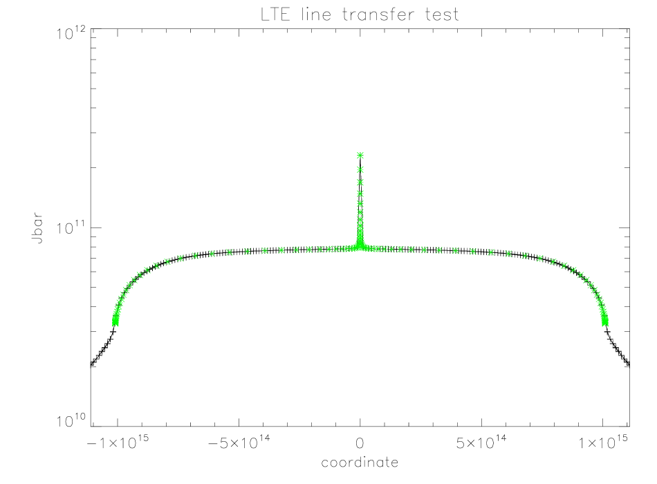
In this test we have set $\epsilon_{l}=1$ to test the accuracy of the formal solution by comparing to the results of the 1D code. The 1D solver uses 64 radial points, distributed logarithmically in optical depth. In Fig. 2 we show the line mean intensities ${\bar{J}}$ as function of distance from the center for both the 1D ($+$ symbols) and the 3D solver. The results plotted in Fig. 1 show an excellent agreement between the two solutions, showing that the line 3D RT formal solution is comparable in accuracy with the corresponding 1D formal solution. Note that the difference of the distribution of spatial points (linear in the 3D case, approximately logarithmic in the 1D case) causes a much lower resolution of the 3D calculations in the central regions and in a higher resolution of the 3D calculations in the outer regions compared to the 1D test case.

3.2 Tests with line scattering

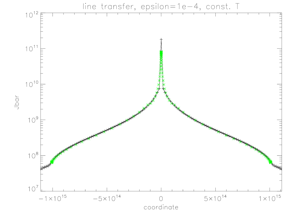
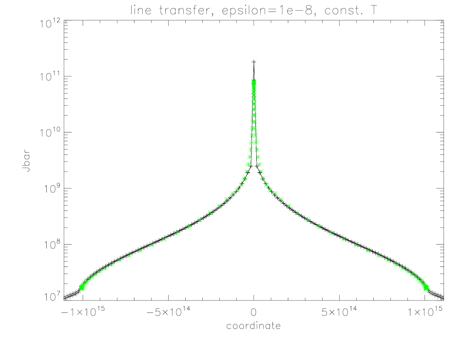
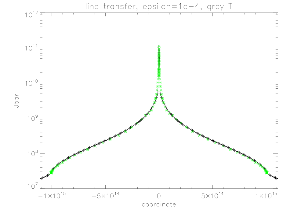
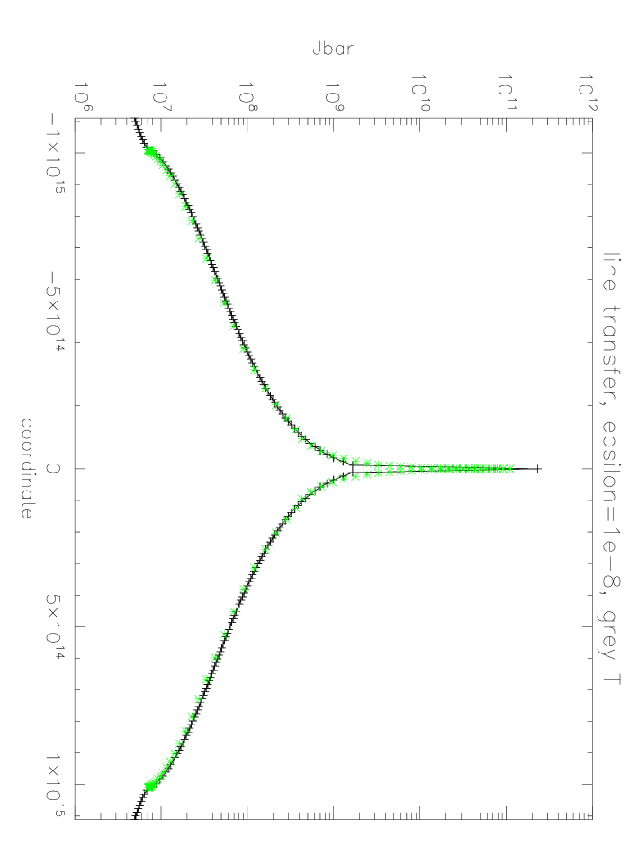
We have run a number of test calculation similar to the LTE case but with line scattering included. In Fig. 3 we show the results for $\epsilon_{l}=10^{-4}$ and in Fig. 4 we show the results for $\epsilon_{l}=10^{-8}$ as examples. In both cases, the dynamical ranges of ${\bar{J}}$ are much larger than in the LTE case. The 3D calculations compare very well to the 1D calculations, in particular in the outer zones. In the inner parts the resolution of the 3D models is substantially lower than for the 1D models, therefore the differences are largest there. In Figs. 3 and 4 we show the results for a test model with a grey temperature structure. In these models, the 3D spatial grid was substantially larger ($n_{x}=n_{y}=n_{z}=2*96+1$) in order to help resolve the inner regions where the temperature gradients are very large. As expected, the agreement is not as good in the inner regions as in the models with a constant temperature, however, the models agree very well in the outer regions. Overall, the agreement is very similar in quality compared to the case with constant temperatures. The differences in the mean intensity $\bar{J}$ between the 1D comparison case and the 3D case is several per-cent in the innermost layers where the grid of the 3D case is under-sampled, the differences are below 0.1% in the outer zones.

3.3 Convergence

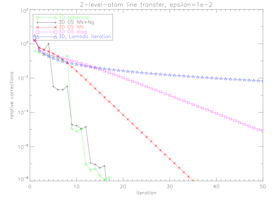
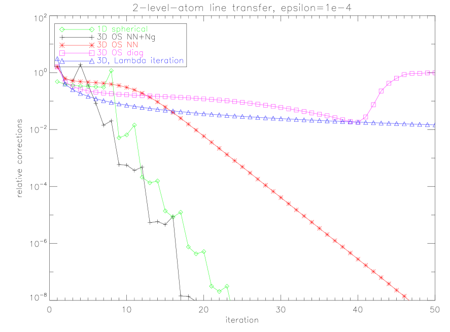
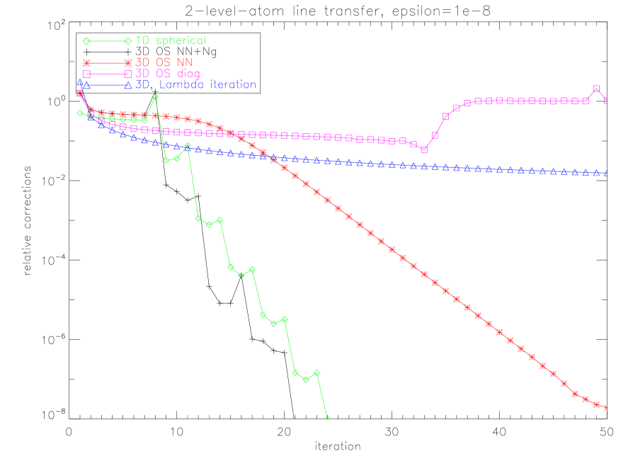
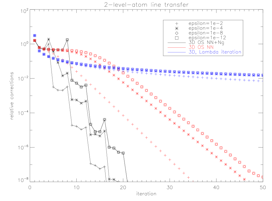
The convergence properties of the line transfer tests presented here are shown in Figs. 7–10. In each figure, we show the convergence rates, as measured by the relative corrections per iteration, for a number of test runs. In all tests show here we have used $n_{x}=n_{y}=n_{z}=2*32+1$ points and $n_{\theta}=n_{\phi}=32$ solid angle points for the 3D test case and 64 radial points for the 1D comparison test. The iterations were started with $S_{l}={\bar{J}}=B$ at all spatial points, this initial guess causes a relative error of about $10$ in ${\bar{J}}$ at the outer zones for the case with $\epsilon_{l}=10^{-2}$ and about $10^{4}$ in ${\bar{J}}$ at the outer zones for the case with $\epsilon_{l}=10^{-8}$. The plots show that the $\Lambda$ iteration is useless even for the relatively benign case of $\epsilon_{l}=10^{-2}$. The operator splitting method delivers much larger corrections and is substantially accelerated by the Ng method, similar to the results shown in Paper I. The nearest-neighbor operator gives substantially better convergence rates than the diagonal operator, cf. Fig 7, for the test cases with with $\epsilon_{l}<10^{-2}$ the convergence behavior of the diagonal operator is unstable, the corrections tend to show oscillations. The nearest-neighbor operator shows stable convergence with quickly declining corrections for all test cases, its convergence rate can be accelerated with Ng’s method. The total number of iterations required for the nearest-neighbor operator is essentially identical to the 1D case with a tri-diagonal operator.

Table 1: Scaling results for different parallel configurations. $N_{\rm worker}$ is the number of MPI processes working on a formal solution for a single wavelength, $N_{\rm cluster}$ is the number of $N_{\rm worker}$ sets of processes working on different wavelength, the total number of MPI processes is $N_{\rm cluster}\times N_{\rm worker}$. The column ’FS+${\Lambda^{*}}$+OS step’ gives teh wallclock time (in seconds) for the calculation of the first formal solution plus the construction of the ${\Lambda^{*}}$ operator plus the time for the first operator splitting step, the column ’FS+OS step’ is the time for the second (and subsequent) formal solution and operator splitting step.

$N_{\rm worker}$	$N_{\rm cluster}$	FS+${\Lambda^{*}}$+OS step	FS+OS step
128	1	3018	1143
64	2	2595	1072
32	4	2340	1032
16	8	2308	1018
8	16	2264	1052
4	32	2318	1054

3.4 Parallelization

We have implemented a hierarchical parallelization scheme on distributed memory machines using the MPI framework similar to the scheme discussed in Baron & Hauschildt (1998). Basically, the most efficient parallelization opportunities in the problem are the solid angle and wavelength sub-spaces. The total number of solid angles in the test models is at least 4096, the number of wavelength points is 32 in the tests presented here but will be much larger in large scale applications. Thus even in the simple tests presented here, the calculations could theoretically be run on 131072 processors. The work required for each solid angle is roughly constant (the number of points that need to be calculated depends on the angle points) and during the formal solution process the solid angles are independent from each other. The mean intensities (and other solid angle integrated quantities) are only needed after the formal solution for all solid angles is complete, so a single collective MPI operation is needed to finish the computation of the mean intensities at each wavelength. Similarly, the wavelength integrated mean intensities ${\bar{J}}$ are needed only after the formal solutions are completed for all wavelengths (and solid angles). Therefore, the different wavelength points can be computed in parallel also with the only communication occurring as collective MPI operations after all wavelength points have been computed. We thus divide the total number of processes up in a number of ‘wavelength clusters’ (each working on a different set of wavelength points) that each have a number of ‘worker’ processes which work on a different set of solid angle points for any wavelength. In the simplest case, each wavelength cluster has the same number of worker processes so that $N_{\rm tot}=N_{\rm cluster}\times N_{\rm worker}$ where $N_{\rm tot}$ is the total number of MPI processes, $N_{\rm cluster}$ is the number of wavelength clusters and $N_{\rm worker}$ is the number of worker processes for each wavelength cluster. For our tests we could use a maximum number of 128 CPUs on the HLRN IBM Regatta (Power4 CPUs) system. In Table 1 we show the results for the 3 combinations that we could run (due to computer time limitations) for a $\epsilon_{l}=10^{-4}$ line transfer test case with 32 wavelength points, $n_{x}=n_{y}=n_{z}=2*64+1$ spatial points and $n_{\theta}=n_{\phi}=64$ solid angle points. For example, the third row in the table is for a configuration with $4$ wavelength clusters, each of them using $32$ CPUs working in parallel on different solid angles, for a total of 128 CPUs. The 3rd and 4th columns give the time (in seconds) for a full formal solution, the construction of the ${\Lambda^{*}}$ operator and an OS step (the first iteration) and the time for a formal solution and an OS step (the second iteration), respectively. As the ${\Lambda^{*}}$ has to be constructed only in the first iteration, the overall time per iteration drops in subsequent iterations. Similarly to the 1D case, the construction of the ${\Lambda^{*}}$ is roughly equivalent to one formal solution. We have verified that all parallel configurations lead to identical results. The table shows that configurations with more clusters are slightly more efficient, mostly due to better load balancing. However, the differences are not really significant in practical applications so that the exact choice of the setup is not important. This also means that the code can easily scale to much larger numbers of processors since realistic applications will require much more than the 32 wavelength points used in the test calculations. Note that the MPI parallelization can be combined with shared memory parallelization (e.g., using openMP) in order to more efficiently utilize modern multi-core processors with shared caches. Although this is implemented in the current version of the 3D code, we do not have access to a machine with such an architecture and it was not efficient to use openMP on multiple single core processors.

4 Conclusions

Using rather difficult test problems, we have shown that our 3D long-characteristics method gives very good results when compared to our well-tested 1D code. The main differences are due to poorer spatial resolution close to the center of the grid in the 3D case. The code has also been parallelized and scales to very large numbers of processors. Future work will examine a short-characteristics method of solution which should enable higher resolution grids with the same memory requirements and an extension to full multi-level NLTE modeling.

Figure 1: Comparison of the results obtained for the LTE line test with the 1D solver ($\times$ symbols) and the 3D line solver. This figure shows cuts along the $x$, $y$, and $z$ axes of the 3D grid for a grid with $n_{x}=n_{y}=n_{z}=2*64+1$ spatial points. The ordinate axis shows the coordinates, the $y$ axis the $\log$ of the mean intensity averaged over the line profiles (${\bar{J}}$) for cuts along the axes of the 3D grid. For the 1D comparison case the ordinate shows $\pm$ distance from the center.

Figure 2: Comparison of the results obtained for the LTE line test with the 1D solver ($+$ symbols) and the 3D line solver. The $x$ axis shows the distances from the center of the sphere, the $y$ axis the $\log$ of the mean intensity averaged over the line profiles (${\bar{J}}$). The 3D model uses $n_{x}=n_{y}=n_{z}=2*64+1$ spatial points.

Figure 3: Comparison of the results obtained for the $\epsilon_{l}=10^{-4}$ line test (constant $T$) with the 1D solver ($\times$ symbols) and the 3D line solver. This figure shows cuts along the $x$, $y$, and $z$ axes of the 3D grid with $n_{x}=n_{y}=n_{z}=2*64+1$ spatial points. The ordinate axis shows the coordinates, the $y$ axis the $\log$ of the mean intensity averaged over the line profiles (${\bar{J}}$) for cuts along the axes of the 3D grid. For the 1D comparison case the ordinate shows $\pm$ distance from the center.

Figure 4: Comparison of the results obtained for the $\epsilon_{l}=10^{-8}$ line test (constant $T$) with the 1D solver ($\times$ symbols) and the 3D line solver. This figure shows cuts along the $x$, $y$, and $z$ axes of the 3D grid with $n_{x}=n_{y}=n_{z}=2*64+1$ spatial points. The ordinate axis shows the coordinates, the $y$ axis the $\log$ of the mean intensity averaged over the line profiles (${\bar{J}}$) for cuts along the axes of the 3D grid. For the 1D comparison case the ordinate shows $\pm$ distance from the center.

Figure 5: Comparison of the results obtained for the $\epsilon_{l}=10^{-4}$ line test (grey $T$) with the 1D solver ($\times$ symbols) and the 3D line solver. This figure shows cuts along the $x$, $y$, and $z$ axes of the 3D grid with $n_{x}=n_{y}=n_{z}=2*96+1$ spatial points. The ordinate axis shows the coordinates, the $y$ axis the $\log$ of the mean intensity averaged over the line profiles (${\bar{J}}$) for cuts along the axes of the 3D grid. For the 1D comparison case the ordinate shows $\pm$ distance from the center.

Figure 6: Comparison of the results obtained for the $\epsilon_{l}=10^{-8}$ line test (grey $T$) with the 1D solver ($\times$ symbols) and the 3D line solver. This figure shows cuts along the $x$, $y$, and $z$ axes of the 3D grid with $n_{x}=n_{y}=n_{z}=2*64+1$ spatial points. The ordinate axis shows the coordinates, the $y$ axis the $\log$ of the mean intensity averaged over the line profiles (${\bar{J}}$) for cuts along the axes of the 3D grid. For the 1D comparison case the ordinate shows $\pm$ distance from the center.

Figure 7: Convergence of the iterations for the line transfer case with $\epsilon_{l}=10^{-2}$. The maximum relative corrections (taken over all spatial points) are plotted vs. iteration number.

Figure 8: Convergence of the iterations for the line transfer case with $\epsilon_{l}=10^{-4}$. The maximum relative corrections (taken over all spatial points) are plotted vs. iteration number.

Figure 9: Convergence of the iterations for the line transfer case with $\epsilon_{l}=10^{-8}$. The maximum relative corrections (taken over all spatial points) are plotted vs. iteration number.

Figure 10: Convergence of the iterations for the line transfer case with different $\epsilon_{l}$ as indicated in the legend. The maximum relative corrections (taken over all spatial points) are plotted vs. iteration number. The symbols without connecting lines are the convergence rates obtained without using Ng acceleration.