Upper limits on the solar-neutron flux at the Yangbajing neutron monitor from BATSE-detected solar flares

Abstract

Aims. The purpose of this work is to search the Yangbajing neutron monitor data obtained between 1998 October and 2000 June for solar neutrons associated with solar flares.

Methods. Using the onset times of 166 BATSE-detected flares with the GOES peak flux (1 – 8 Å) higher than $1.0\times 10^{-5}$ $\mathrm{Wm^{-2}}$, we prepare for each flare a light curve of the Yangbajing neutron monitor, spanning $\pm$ 1.5 hours from the BATSE onset time. Based on the light curves, a systematic search for solar neutrons in energies above 100 MeV from the 166 flares was performed.

Results. No statistically significant signals due to solar neutrons were found in the present work. Therefore, we put upper limits on the $>$ 100 MeV solar-neutron flux for 18 events consisting of 2 X and 16 M class flares. The calculation assumed a power-law shaped neutron energy spectrum and three types of neutron emission profiles at the Sun. Compared with the other positive neutron detections associated with X-class flares, typical 95% confidence level upper limits for the two X-class flares are found to be comparable to the lowest and second lowest neutron fluxes at the top of the atmosphere. In addition, the upper limits for M-class flares scatter in the range of $10^{-2}$ to 1 neutrons $\mathrm{cm^{-2}s^{-1}}$. This provides the first upper limits on the solar-neutron flux from M-class solar flares, using space observatories as well as ground-based neutron monitors.

1 Introduction

Solar neutrons as well as nuclear gamma rays have been widely used as a good probe to the still unclear fundamental mechanisms of ion acceleration associated with solar flares. These neutral secondaries emanate deep in the chromosphere via nuclear processes between accelerated ions and the solar ambient plasma.

Early quantitative studies (Hess 1962; Lingenfelter et al. 1965a, b; Lingenfelter 1969) predicted that large solar flares would produce a measurable flux of solar neutrons at the Earth, $\sim$ 10 $\mathrm{cm^{-2}s^{-1}}$, in energies above 10 MeV. Before the solar cycle 21, various balloon-borne experiments attempted to detect the predicted neutrons originating from solar flares (Apparao et al. 1966; Daniel et al. 1967; Hess & Kaifer 1967; Daniel et al. 1969; Forrest & Chupp 1969), but none gave convincing results.

In the solar cycle 21 and 22, the predicted solar neutrons have actually been detected from several X-class solar flares by satellite-borne or ground-based detectors (Chupp et al. 1982, 1987; Muraki et al. 1992; Debrunner et al. 1993; Struminsky et al. 1994). The first clear detection was achieved with the Gamma-Ray Spectrometer (GRS) on board the Solar Maximum Mission (SMM), on the occasion of an X2.6 solar flare on 1980 June 21 (Chupp et al. 1982). On the other hand, all ground-based positive detections were associated with more energetic solar flares, with the GOES class larger than X8. While these successful detections indeed demonstrated the production of solar neutrons in solar flares, it was thought that the neutron detection from medium X-class flares would be difficult with ground-based observations.

Surprisingly, solar neutrons were successfully detected from an X2.3 solar flare on 2000 November 24, at near the maximum of the solar cycle 23, by a neutron monitor installed at Mt. Chacaltaya in Bolivia (Watanabe et al. 2003). The Bolivian neutron monitor is situated at an altitude of 5250 m and has an area of 13 $\mathrm{m^{2}}$. This observation therefore inspired that ground-based detectors at very high mountains would be able to detect solar neutrons even from medium X-class solar flares, although the 2000 November 24 event might be exceptional.

Because of the small ($\sim$10) number of positive detections of solar neutrons, it is not clear at present how the arrival flux of solar neutrons depends on the flare intensity. Furthermore, it is unlikely that the neutron detections will increase in number significantly in near future. Therefore, we may utilize even upper limits on the solar-neutron flux for a much larger sample of solar flares. These upper limits at the Earth are expected to constrain some key parameters of the underlying ion acceleration process in solar flares, including the total number, the energy content, and pitch angle distributions of the accelerated ions. In the present paper, we hence analyze the data from the Yangbajing neutron monitor for any signals associated with 166 M- and X-class flares, detected with the BATSE (Burst And Transient Source Experiment) on board Compton Gamma Ray Observatory (CGRO) over a period of 1998 October through 2000 June.

In Section 2 we give an overview of the Yangbajing neutron monitor, and describe in Section 3 its performance using Monte Carlo simulations. Section 4 presents our methods used in this analysis. The derived results are given in Section 5, together with a brief discussion.

2 The Yangbajing neutron monitor

The Yangbajing neutron monitor (NM) has been operated at Yangbajing ($90{\degr}.522$E, $30{\degr}.102$N) in Tibet, China, since 1998 October (Kohno et al. 1999; Miyasaka et al. 2001). Its high altitude, 4300 m above sea level, provides a much reduced air mass, 606 $\mathrm{gcm^{-2}}$. It consists of 28 NM64 type detectors (Carmichael 1964; Stoker et al. 2000), attaining a total area of 31.7 $\mathrm{m^{2}}$ which is the largest one among the world-wide NM network at present. Another advantage of the Yangbajing NM is that it has the highest geomagnetic cutoff rigidity, 14 GV, among NMs in the world, thanks to geomagnetic conditions. These conditions make the Yangbajing NM one of the most sensitive detectors for solar neutrons.

3 Performance of the Yangbajing neutron monitor

The data acquisition system of the Yangbajing NM records the event number of each counter every second. The counting rate is typically 100 Hz per counter, so the total rate becomes around 2.8 kHz. In order to examine whether this value is reasonable, we calculated the expected counting rate of the Yangbajing NM by means of a full Monte Carlo (MC) simulation in the atmosphere called Cosmos uv6.35 (Kasahara 2003). Primary cosmic-ray particles were sampled from the energy spectrum constructed from direct observations in the energy range from 10 GeV to 100 TeV (Asakimori et al. 1998; Sanuki et al. 2000; Apanasenko et al. 2001; Sanuki et al. 2001). An error of $\pm 20$% was assigned to the absolute flux of primary particles in lower energies, whereas its uncertainty was set to be $\pm 50$% at around 100 TeV. These primary particles were thrown isotropically within the zenith angle $0\degr$ to $60\degr$ on top of the atmosphere, and then fluxes of various secondary particles at the altitude of Yangbajing were evaluated. The flux of species of each secondary particle was finally multiplied by the detection efficiency of the NM64 detector calculated by Clem & Droman (2000), which in turn was confirmed via comparison with an accelerator experiment using 100 $-$ 400 MeV neutron beams (Shibata et al. 2001).

As a consequence of the calculation, the expected counting rate of the Yangbajing NM was estimated as 3.4 kHz. This is in agreement with the experimental counting rate of 2.8 kHz within the error of the absolute flux of primary particles. In addition, the MC simulation revealed how various secondary particle species contribute to the total counting rate. The secondary neutrons were found to dominate the counting rate with a typical fraction of 83%. The next dominant contribution comes from protons, 15% to the total counting rate. The remaining marginal 2% is mainly due to secondary negative muons that are captured in the lead blocks through a reaction of $\mu^{-}+\mathrm{p}\rightarrow\mathrm{n}+\nu_{\mu}$. This result ensures that 98% of the counting rate is dominated by secondary nucleons, as expected.

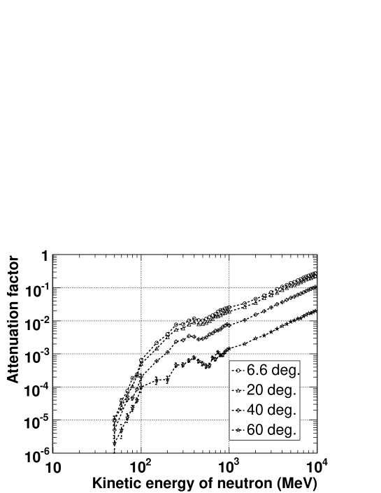
Figure 1: The atmospheric attenuation factor of solar neutrons, calculated via Monte-Carlo simulations assuming different incident zenith angles, and shown as a function of kinetic energy of neutrons measured at the top of the Earth atmosphere.

For a further analysis, we also derived an attenuation factor of solar neutrons in the atmosphere. The attenuation of solar neutrons is caused by their collisions with atmospheric nuclei during their propagation to the observers, depending on their kinetic energies and incident angles. This is illustrated in Fig. 1, which was obtained using MC simulations of CORSIKA 6.500 (Heck et al. 1998) embedding GHEISHA (Fesefeldt 1985; Cassell & Bower 2002) as a low-energy ($<$ 80 GeV/n) hadronic interaction model. Thus, low-energy solar neutrons are strongly reduced in flux, particularly when the incident zenith angle is large. For example, solar neutrons with a kinetic energy of 100 MeV and an incident angle of $60{\degr}$ suffer heavy attenuation by four orders of magnitude. Even with such a heavy attenuation, we expect successful detections of solar neutrons with the Yangbajing NM, if the arriving neutron flux exceeds $\sim 1\mathrm{cm^{-2}s^{-1}}$ as found in some past solar flares with the GOES class above X10, and if each event lasts typically $\sim$ 10 minutes.

4 Analysis

4.1 Flare sample definition

Since the beginning of its operation on 1991 April 19 through the reentry to the atmosphere on 2000 June 4, the BATSE aboard CGRO observed more than 7,000 solar flares in the hard X-ray range above $\sim$ 25 keV; the flare list is publicly available. Among them, 1205 events were detected over a period of 1998 October and 2000 June, i.e., overlapping with the Yangbajing NM operation, with the GOES peak flux ($F_{\mathrm{GOES}}$) higher than 1.0 $\times 10^{-6}$ $\mathrm{Wm^{-2}}$ which corresponds to the GOES class of C1. The flare number reduces to 1013 when we exclude those events of which the Yangbajing NM did not operate due to maintenance or system troubles. The 1013 events, composed of 847 C-class, 159 M-class, and 7 X-class flares, constitute our “very preliminary sample”, which is further divided into two subsets. One subset is called “preliminary sample”, consisting of the 166 flares with the GOES class larger than M1. The other is “sub-preliminary sample”, with the 847 C-class flares.

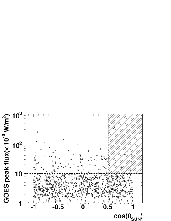
Figure 2: The cosine of the zenith angle of the Sun ($\theta_{\mathrm{SUN}}$) at Yangbajing at the onset time of each flare in our very preliminary sample, plotted against their GOES peak flux in units of $10^{-6}$ $\mathrm{Wm^{-2}}$. The vertical dashed line indicates $\theta_{\mathrm{SUN}}=60{\degr}$, while the horizontal one represents the GOES flux of 1 $\times 10^{-5}$ $\mathrm{Wm^{-2}}$, or the GOES class of M1. The 18 events in the hatched area constitute our final sample.

As indicated by Fig. 1, the zenith angle of the Sun at Yangbajing, $\theta_{\mathrm{SUN}}$, must be small in order for the Yangbajing NM to detect neutron signals. Therefore, we arranged the 1013 “very preliminary” sample events, in Fig. 2, on the plane of $\cos(\theta_{\mathrm{SUN}})$ calculated at the flare onset vs $F_{\mathrm{GOES}}$. Based on this plot, we have selected 18 flares for our “final sample”, with criteria that $\theta_{\mathrm{SUN}}$ is smaller than $60{\degr}$ and $F_{\mathrm{GOES}}$ is higher than 1.0 $\times 10^{-5}$ $\mathrm{Wm^{-2}}$. These flare are summarized in Table 1.

4.2 NM light curves

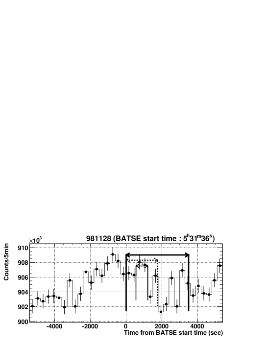
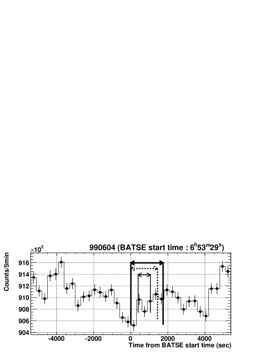
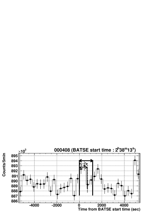
Figure 3: The 5-minute counting-rate histories of the Yangbajing NM for two X-class and two M-class flares. Top and second panels show light curves for an X3.7 (981122) and X3.3 (981128) flares, respectively, while third and bottom panels indicate those for an M3.9 (990604) and M2.0 (000408) flares, respectively. Abscissa in all panels shows the time measured from $t_{\mathrm{S}}$, ranging over $\pm$ 5400s, where zero corresponds to the BATSE start time (Table 1). The intervals of individual ON time windows specified by the $\delta$-, continuous-, and gaussian-emission profiles are indicated by horizontal thin, thick, and dashed arrows, respectively. The errors indicate uncorrected $1\sigma$ statistical ones, simply calculated by square root of each 5-minutes counts.

Our basic strategy is to search the NM count-rate histories (or “light curves”) for possible excess counts associated with solar flares. For each flare in our preliminary sample, we therefore prepared a light curve from the Yangbajing NM, spanning $\pm$ 1.5 hours from the flare onset time, $t_{\mathrm{S}}$, determined by the BATSE data. This time interval is considered long enough to cover each flare, and to estimate background count levels. We binned the light curves into 5 minutes per bin, and corrected them for atmospheric pressure changes which cause variations in the attenuation factor by typically $\pm$2%. Figure 3 shows four particular examples of such light curves out of the 18 final-sample flares; these are two X-class flares, 981122 and 981128, and two M-class ones, 990604 and 000408, with the latter two being the highest and the second highest BATSE peak rates among M-class flares in our final sample (Table 1). Thus, no excess counts due to solar neutrons are apparently observed.

In order to more quantitatively constrain neutron counts associated with each flare, we need to define for each flare an “ON time window”, i.e., a time interval when solar neutrons might indeed arrive at the Yangbajing NM, and use the remaining two time intervals (before and after the flare) to estimate the background. For this purpose, we must in turn assume a time profile of the solar-neutron production at the Sun in each flare, as well as the maximum and minimum kinetic energies of the produced solar neutrons. Then the “ON time window”opens at the arrival of the most energetic neutrons ejected at the beginning of the neutron emission at the Sun, and closes at that of the least energetic ones ejected at the end of the production interval. In this work, we postulate that the maximum and minimum kinetic energies of solar neutrons are 10 GeV and 100 MeV, respectively.

The following three neutron-emission time profiles are employed; (1) $\delta$-emission, (2) continuous-emission, and (3) gaussian-emission. the $\delta$-emission simply means that solar neutrons are emitted from the Sun instantaneously at the BATSE HXR emission peak, while the continuous-emission profile assumes that neutrons are continuously and constantly radiated from the Sun throughout the BATSE HXR emission. Here for the purpose of introducing mathematical forms of each emission profile, we define “re-normalizing” time $t$ as $T-t_{\mathrm{S}}$, where $T$ and $t_{\mathrm{S}}$ show the normal time measured in UT and the onset time of the BATSE emission, respectively. With the renormalizing time $t$ and above assumptions, the neutron emission profile $\nu(t)$ takes either of the following forms; $\nu(t)=1$ only at $t=t_{\mathrm{P}}-t_{\mathrm{S}}$ and otherwise 0 if the $\delta$-emission is adopted, $\nu(t)=1$ for $t=$ 0 to $\Delta t_{\mathrm{b}}$ and otherwise 0 if the continuous-emission profile is used. Here, $t_{\mathrm{P}}$ is the peak time of the BATSE emission, and $\Delta t_{\mathrm{b}}$ is the BATSE flare duration. Hereafter we define $T_{\mathrm{PS}}=t_{\mathrm{P}}-t_{\mathrm{S}}$. Both these cases have been considered in some past studies (Chupp et al. 1982; Muraki et al. 1992; Shibata 1994; Watanabe et al. 2003; Bieber et al. 2005).

In comparison with these simplified emission profiles, the gaussian-emission profile is a rather realistic one, defined as

$$\nu(t)=\left\{\begin{array}[]{ll}C\exp\left({-(t-T_{\mathrm{PS}})^{2}/2\Delta T^{2}}\right)&\mbox{if $0\leq t\leq 2T_{\mathrm{PS}}$},\\ 0&\mbox{otherwise},\end{array}\right.,$$ (1)

where $C$ is a normalization factor so that time integral of $\nu(t)$ over 0 – $2T_{\mathrm{PS}}$ is unity, and its centroid and standard deviation $\Delta T$ are set to be $T_{\mathrm{PS}}$ and $0.5T_{\mathrm{PS}}$, respectively. This is because that light curves of the 4 – 7 MeV nuclear gamma-ray emission, which obviously reflect ion acceleration at the Sun, is approximately described by a Gaussian function (e.g., Chupp et al. 1990; Watanabe et al. 2003). Furthermore, according to various solar X-ray and gamma-ray observations (e.g., Forrest & Chupp 1983; Watanabe et al. 2006), the rise and peak times of the 4 – 7 MeV nuclear gamma-ray light curve are roughly similar to those of the HXR emission.

In this work we treat three neutron emission profiles, since it is natural that ions are accelerated in solar flares at the same time as electrons. However, a recent work performed by Sako et al. (2006) suggests that acceleration time or trapping time of ions in 2005 September 7 flare may be longer than that of electrons. Thus, it should be noted that we might expect more arrival neutron flux than the following investigation.

The ON time windows specified by these three profiles are illustrated in Fig. 3. Here we give a brief explanation of the ON time windows, using 981122 flare (top panel of Fig. 3) as an example. Since the $\delta$-emission supposes instantaneous neutron emission at the Sun, the corresponding ON time window starts at $t_{\mathrm{P}}+1.85$ s and end at $t_{\mathrm{P}}+667$ s, lasting for 665 s, where 1.85 s and 667 s are time delays of 10 GeV and 100 MeV neutrons, respectively, with respect to photons. Since this flare has $T_{\mathrm{PS}}=341$ s, the ON time windows lasts from 343 s to 1008 s as measured from $t_{\mathrm{S}}$. The ON time windows specified by the other two models are longer than that by the $\delta$-emission, because these assume prolonged neutron emissions. It should be stated that 5-minute counts shown in Fig. 3 seem to be highly variable. This is because normal Poisson error is assigned to each count. In order to explain that the variations are not so large, we introduce a correction factor for errors of 5-minute counts in Section 4.3.

By excluding all count bins in the ON time window and two adjacent count bins, two time regions are available in each light curve for background estimation. We then determined the background level of the NM counts, by fitting a common quadratic curve to these two time windows through a least square method. The calculated quadratic curve in turn enables us to define the background level inside the ON time window. This removes residual temporal trend (such as seen in the 3-hours data of Fig. 3), mostly due to solar diurnal variation with a typical amplitude of $\pm$ 0.3%; this arises from diffusion and convection of Galactic cosmic-rays below several tens GeV in the interplanetary space (e.g., Parker 1965; Jokipii & Parker 1970). Finally, all counts in the ON time window are summed up (hereafter $N_{\mathrm{ON}}$), and all the interpolated background counts in the same ON time window are likewise accumulated (hereafter $N_{\mathrm{BG}}$). Then the signal from solar neutrons in the ON time window, $N_{\mathrm{S}}$, is available by simply subtracting $N_{\mathrm{BG}}$ from $N_{\mathrm{ON}}$. Here the $N_{\mathrm{S}}$ would probably correspond to the “worst” neutron signals since we equally treat all counts in an ON time window as neutron signals. Practically, more neutron signals could be expected via optimizing an ON time window for any emission models. This is our future work.

4.3 Significance of the neutron signal

For the purpose of calculating the statistical significance of $N_{\mathrm{S}}$, we need to estimate its uncertainty $\Delta N_{\mathrm{S}}$ given by $\sqrt{\Delta N_{\mathrm{ON}}{}^{2}+\Delta N_{\mathrm{BG}}{}^{2}}$, where $\Delta N_{\mathrm{ON}}$ and $\Delta N_{\mathrm{BG}}$ represent errors associated with $N_{\mathrm{ON}}$ and $N_{\mathrm{BG}}$, respectively. However these quantities do not obey Poisson statistics, since the lead blocks, used to increase the detection efficiency through multiplication of incident neutrons, often lead to multiple counts in the $\mathrm{BF_{3}}$ counter for one incident neutron. This prevents us from estimating, e.g., simply as $\Delta N_{\mathrm{ON}}=\sqrt{N_{\mathrm{ON}}}$. Therefore, using the NM data themselves, let us derive a correction factor $\Gamma(>1)$ which yields $\Delta N_{\mathrm{ON}}=\Gamma\sqrt{N_{\mathrm{ON}}}$.

We first constructed occurrence histograms of the 5-minutes counts each day, excluding those data which were obtained during 3 days after the occurrence of a preliminary-sample flare. This is to avoid possible flare-associated effects, such as the arrival of solar energetic charged particles and/or a subsequent Forbush decrease. The produced histograms are refereed to collectively as “background-histogram sample”. Then each histogram in the background-histogram sample is fitted with a Gaussian function, in order to derive its mean value, $\mu$, and standard deviation, $\sigma$, and to consequently obtain the factor $\Gamma=\sigma/\sqrt{\mu}$. Here such a multiplicity in NMs was firstly discussed by Carmichael (1964).

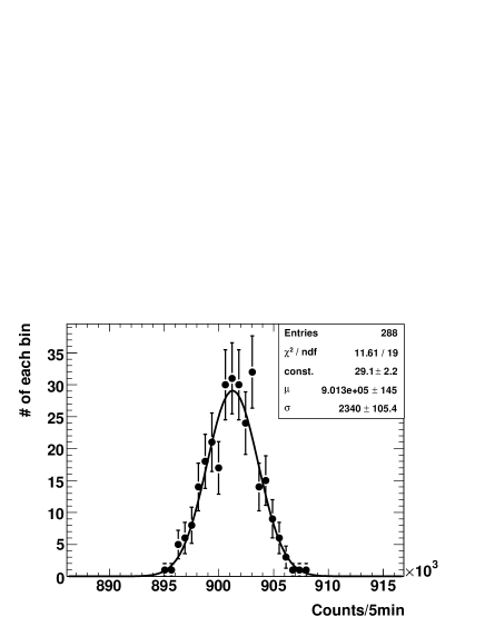
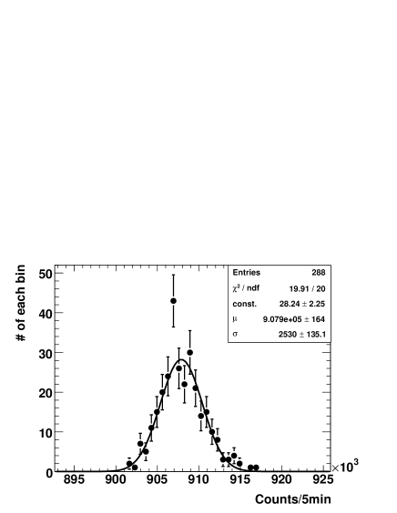
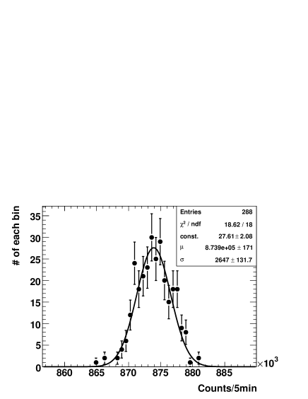
Figure 4: Typical occurrence histograms of the 5-minutes counts of the Yangbajing NM data on 1998 December 3 (top), 1999 June 3 (middle), and 2000 April 30 (bottom). Error bars assigned to individual data points are Poissonian $\pm 1\sigma$. The solid line indicates the best Gaussian fit to each distribution.

Figure 4 shows some typical distributions in the background-histogram sample. Since the distribution of top panel of Fig. 4 has $\mu=901270\pm 145$ and $\sigma=2340\pm 105$, both per 5 minutes, we find that $\sigma$ deviates from the expected Poisson fluctuation, $\sqrt{\mathrm{\mu}}$, by a factor of $\Gamma=2340/\sqrt{901270}=2.46\pm 0.11$. The other distributions shown in Fig. 4 also exhibit similar excess above the expected Poisson fluctuation, yielding $\Gamma=2.65\pm 0.14$ (middle panel) and $2.83\pm 0.14$ (bottom panel). Deriving the factor $\Gamma$ from each histogram in the background-histogram sample in the same way, and averaging them over the analyzed period, we obtained the averaged correction factor as $\Gamma=2.73\pm 0.01$. Furthermore, the standard deviation in 5-minutes counts has been estimated as $\sigma^{*}=2576\pm 16$. As can be seen from the particular examples of Fig. 4, the mean $\mu$ varies by $\pm 10-20$% from day to day, due, e.g., to monthly and yearly solar activity changes. The factor $\Gamma$ also varies by a similar extent, depending on the day. However we regard $\Gamma$ as constant, because the fluctuations in $\Gamma$ do not affect our final results. Here, as a general remark, a recent study for NM multiplicity given by  Bieber et al. (2004) has suggested that the multiplicity for a 100 MeV neutron are relatively larger than the derived value in this work. Probably, the difference may result from some systematic differences such as logic of electronics, arrangement of NMs, and geophysical conditions of a station.

Using $\Gamma$ as calculated above, $\Delta N_{\mathrm{ON}}{}^{2}$ is determined as $\sum(\Gamma\sqrt{N_{\mathrm{cnt}}})^{2}=\Gamma^{2}N_{\mathrm{ON}}$, where summation is done over an ON time window, while $\Delta N_{\mathrm{BG}}{}^{2}$ is evaluated as $\sum(\sigma^{*}/\sqrt{n_{\mathrm{off}}})^{2}$, where summation is also performed over the ON time window and $n_{\mathrm{off}}$ is the number of 5-minutes bins used to define the background level through the least square method. Finally, the significance of possible neutron signals, $\sigma_{\mathrm{S}}$, can be calculated as

$$\sigma_{\mathrm{S}}=\frac{N_{\mathrm{ON}}-N_{\mathrm{BG}}}{\sqrt{\Gamma^{2}N_{\mathrm{ON}}+\sum(\sigma^{*}/\sqrt{n_{\mathrm{off}}})^{2}}}.$$ (2)

5 Results and discussions

5.1 Significance distributions

With equation (2), we calculated the statistical significances of the 18 final-sample flares. Table 2 summarizes the values of $\sigma_{\mathrm{S}}$, for the three neutron production profiles, together with $N_{\mathrm{S}}$ and $\Delta N_{\mathrm{S}}$. Thus, the signal significance is at most $2\sigma$, implying all null detections. Then, how about the other flares ?

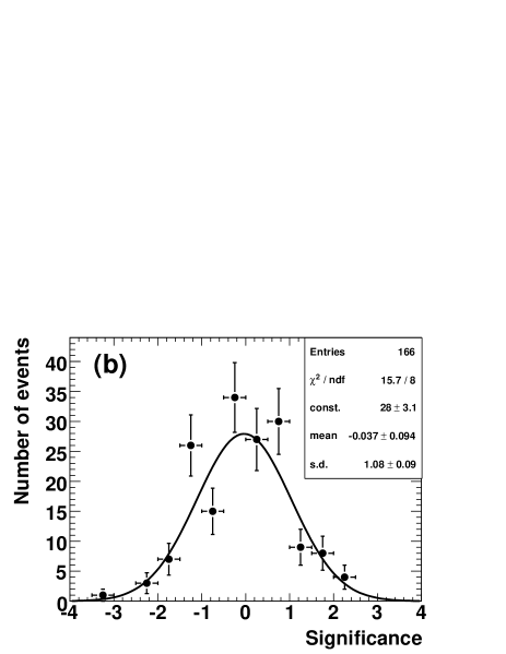
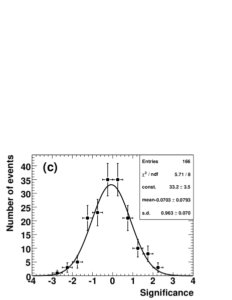
Figure 5: Significance distributions of neutron signals from our preliminary-sample flares, computed assuming the three neutron-emission profiles. Panels (a), (b), and (c) correspond to the $\delta$-, continuous-, and gaussian-emission models, respectively. Vertical error bars associated with individual data points are Poissonian. The best-fit gaussian curve to each histogram is drawn by a solid line. Statistical parameters obtained from each fit are indicated in the legend of each graph.

Figure 5 shows occurrence histograms of the statistical significance of signal neutron counts of our preliminary-sample flares, calculated with equation (2) in the same way. The 166 flares have been binned into appropriate intervals. We fitted each histogram in Fig. 5 with a Gaussian distribution, with its height, mean value, and standard deviation left free. The fit has been successful as shown in Fig. 5, with two important consequences. One is that the obtained Gaussian centroids are consistent with 0 within the fitting errors. Therefore, there is no evidence, in the statistical sense, for positive neutron signals associated with the 166 solar flares. The other point is that the obtained standard deviations are consistent with 1.0, implying that the significance scatter among the 166 flares can be fully explained by statistical fluctuations and that the value of $\Gamma$ has been correctly estimated. The latter fact also ensures that the developed method is not affected significantly by any unknown systematic effects. For clarifying this, other analysis were performed, systematically including one bin before the beginning of the BATSE start time or leaving out the last bin in ON time windows. The difference between the obtained results shown in Fig. 5 and those other results can be well explained by statistical fluctuation.

5.2 Calculation of an upper limit of the solar-neutron flux

Given the null detections of solar neutrons, we proceed to set upper limits on the solar-neutron flux from the 18 final-sample flares (Table 1). For this purpose, an upper limit on the neutron counts at 95% confidence level (CL), $N_{95}$, was estimated for each final-sample flare, from the ON time window counts $N_{\mathrm{S}}$ and its uncertainty $\Delta N_{\mathrm{S}}$, and using a statistical method by Helene (1983). The obtained results on $N_{95}$ are provided in Table 2.

The quantity $N_{95}$ may be written as

$$N_{95}=R^{-2}\int^{\Delta t_{\mathrm{b}}+T_{\mathrm{max}}}_{0}\!\!\!dt\int^{T_{\mathrm{max}}}_{T_{\mathrm{min}}}\!\!\!\nu(t-t^{\prime})N(E_{\mathrm{n}})P(E_{\mathrm{n}})A(\theta,E_{\mathrm{n}})\frac{dE_{\mathrm{n}}}{dt^{\prime}}dt^{\prime}.$$ (3)

Here, $R$ is the distance from the Sun to the Earth; $t$ is the time measured from $t_{\mathrm{S}}$; $\Delta t_{\mathrm{b}}$ is again the BATSE duration; the times $T_{\mathrm{min}}$ and $T_{\mathrm{max}}$ correspond to delays of 10 GeV and 100 MeV solar neutrons, respectively; the variable $t^{\prime}$ is the difference between the Sun-Earth transit times for neutrons and photons; $E_{\mathrm{n}}$ is the kinetic energy of neutrons which is a function of $t^{\prime}$; and $\theta$ is the incident angle of neutrons at the top of the atmosphere, which is $\theta_{\mathrm{SUN}}$ in Table 1. Furthermore, $\nu$ is the neutron production time profile defined in Section 4.2, $N(E_{\mathrm{n}})$ is the differential neutron spectrum at the Sun, $P(E_{\mathrm{n}})$ is the probability for a neutron to reach the Earth before its decay, and $A(\theta,E_{\mathrm{n}})$ is the effective area of the Yangbajing NM which is a product of the atmospheric attenuation factor (Fig. 1) and the detection efficiency of an NM64 detector (Clem & Droman 2000). The term $dE_{\mathrm{n}}/dt^{\prime}$ is the neutron energy-time dispersion relation (Lingenfelter & Ramaty 1967). We assume the function $N(E_{\mathrm{n}})$ to have a form of $\alpha(E_{\mathrm{n}}/100$ $\mathrm{MeV})^{-\beta}$ $(\mathrm{sr^{-1}MeV^{-1}})$, which is theoretically expected from the shock acceleration process of ions in solar flares (see Hua et al. 2002, and references therein). Here, the power-law index $\beta$ is assumed to take values of 3, 4, and 5 as conservative ones (Chupp et al. 1987; Muraki et al. 1992; Struminsky et al. 1994; Watanabe et al. 2003, 2006). Since $\theta$ varies from flare to flare (Table 1), $A(\theta,E_{\mathrm{n}})$ is interpolated from effective areas calculated for a set of incident angles of $6.6{\degr}$, $10{\degr}$, $20{\degr}$, $30{\degr}$, $40{\degr}$,$50{\degr}$, and $60{\degr}$.

On the right hand side of equation (3), the only unknown quantity is the spectrum normalization $\alpha$. Therefore, by substituting the measured values of $N_{95}$ (Table 2) for the left hand side of equation (3), we can determine $\alpha$ for each flare. We can then calculate a 95% CL upper limit on the neutron flux at the top of the Earth atmosphere as

$$F_{95}=\alpha\Delta T_{\mathrm{n}}^{-1}R^{-2}\int^{\Delta t_{\mathrm{b}}+T_{\mathrm{max}}}_{0}\!\!\!dt\int^{T_{\mathrm{max}}}_{T_{\mathrm{min}}}\!\!\!\nu(t-t^{\prime})(E_{\mathrm{n}}/100\mathrm{MeV})^{-\beta}P(E_{\mathrm{n}})\frac{dE_{\mathrm{n}}}{dt^{\prime}}dt^{\prime},$$ (4)

where $\Delta T_{\mathrm{n}}$ is the time interval of the ON time window. The inner integral of the right hand side of equation (4) differs from that of equation (3) in that the effective area $A(\theta,E_{\mathrm{n}})$ has been eliminated.

5.3 The flux upper limits of the final-sample flares

Figure 6 and Table 3 show the upper limits on the $>$ 100 MeV solar-neutron flux, $F_{95}$ calculated with equation (4), for the two (X3.7 and X3.3) of our final sample flares. For comparison, the previous positive detections (Ramaty et al. 1983; Chupp et al. 1987; Evenson et al. 1990; Muraki et al. 1992; Debrunner et al. 1993; Struminsky et al. 1994; Debrunner et al. 1997; Watanabe et al. 2003; Bieber et al. 2005; Watanabe et al. 2006) are also plotted. Here, the horizontal axis in Fig. 6 gives the GOES class, and hence the values of 1 and 10 correspond to the GOES class of X1 and X10, respectively. As can be easily seen from Fig. 6, the present two upper limits are comparable with the lowest neutron flux derived from the SMM observation (Chupp et al. 1982) and second lowest one from the highest-altitude NM observation (Watanabe et al. 2003). These upper limits, therefore, provide rather stringent constraints on the neutron flux from medium X-class flares, even though they were observed at large zenith angles of $\sim 50\degr$ (Table 1).

As shown in Fig. 6, a positive correlation between absolute neutron fluxes and GOES class is expected. The derived upper limits are also not inconsistent with such a expected correlation. Using those absolute fluxes, Fig. 6 reveals a relatively tight and steep dependence of the solar neutron flux on $F_{\mathrm{GOES}}$. In fact, the correlation is quantitatively represented as $F_{\mathrm{n}}\propto F_{\mathrm{GOES}}{}^{3.0\pm 0.2}$ (The error of the power-law index is statistical only). Since the dependence is considerably steeper than direct proportionality, it is strongly suggested that a larger flare not only accelerates a larger number of nucleons, but also accelerates them to higher energies.

SMM observations of 19 X-class flares, ranging from X1 to X20, have provided a sample of 0.8 – 7 MeV nuclear gamma-ray fluxes at the top of the Earth atmosphere (Share & Murphy 1995). Using the sample, we examined in the same way how the nuclear gamma-ray flux depends on $F_{\mathrm{GOES}}$. As a result, the dependence was found to be much weaker than that of the neutron flux, quantitatively given as $F_{\gamma}\propto F_{\mathrm{GOES}}{}^{0.32\pm 0.02}$ (The error is also statistical only). Thus, the dependence of both secondaries related to ion acceleration on $F_{\mathrm{GOES}}$ is greatly different, at least, within the quoted statistical errors. The difference between the two relations might be in part attributed to a difference in characteristic ion energies responsible for these emissions: nuclear gamma rays are produced primarily by accelerated ions with energies of 1 – 100 MeV/n, while 10 – 100 MeV/n or even higher-energies are necessary for the accelerated ions to efficiently produce high-energy solar neutrons with a detectable flux on the ground (Mandzhavidze & Ramaty 1993; Aschwanden 2002).

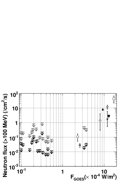
Figure 7: The same as Fig. 6, but including all the final sample flares. Each black arrow shows the most stringent upper limit for each final sample flare, while the least stringent ones are indicated by gray arrows. The detail information on each data point are shown in the caption of Fig. 6.

In order to further examine the relation between the solar-neutron flux and the flare intensity, we show in Fig. 7 all upper limits from the final sample flares, and give numerical values of the most and the least stringent upper limits in Table 4. The most stringent upper limits in the present work are obtained assuming that $\beta$ is 3 and $\nu(t)$ is the continuous-emission, while the least stringent ones are derived assuming that $\beta$ is 5 and $\nu(t)$ is the $\delta$-emission. From the most stringent upper limits, it is found that the neutron flux of M-class flares are probably below 0.01 $\mathrm{cm^{-2}s^{-1}}$ at one AU. This is consistent with the fact that neither space observatories nor ground-based detectors have so far succeeded in detecting solar neutrons from M-class solar flares.

5.4 Dependence on propagation models

Finally, we examine how our upper limits depend on propagation models used to calculate the atmospheric attenuation factors of solar neutrons. Presently, several kinds of hadronic interaction models are available to deal with complicated nuclear reactions in energies below 10 GeV. Among them, the present work has employed GHEISHA in CORSIKA 6.500. However, another model developed by Shibata (1994) has been widely known as one of the representative solar neutron propagation models, because MC simulations based on the Shibata model well reproduce experimental results using 100 – 400 MeV neutron beams (Koi et al. 2001; Tsuchiya et al. 2001). Thus, a comparison between GHEISHA and the Shibata model should be carried out.

Using the 981122 (X3.3) and 981128 (X3.7) flares as representative, we computed the flux upper limits using the Shibata model, and compared the results with those from GHEISHA in Table 5. Thus the upper limits based on the Shibata model are about a quarter of those based on GHEISHA. Therefore, this factor should be considered as another systematic uncertainty involved in our results. Since every solar neutron observations on ground is affected by this uncertainty, we must use the same propagation model if trying to compare different observations.

6 Summary and further prospects

So far, the solar neutron observations and subsequent analyses have exclusively noticed X-class flares. However, to understand ion acceleration in solar flares, it is very important to examine how the solar neutron flux depends on the flare intensity. For this purpose, we systematically searched the Yangbajing NM data, taken from 1998 October to 2000 June, for solar neutrons, focusing on 166 BATSE-detected M and X-class flares. No statistically significant signals were found from our small final sample consisting of 2 X-class flares and 16 M-class ones. Hence, the 95% confidence level upper limits on the $>$ 100 MeV neutron flux were derived for individual flares. As a consequence, it was found that the upper limits for the two medium X-class flares are comparable with the neutron flux evaluated from the positive detections by the SMM satellite and the highest-altitude NM. These results suggest a very steep dependence of the solar neutron flux on the flare size. Furthermore, we for the first time derived useful upper limits on the solar neutron flux from M-class flares.

Some experiments with newly developed high sensitive detectors are proposed for space missions (Imaida et al. 1999; Moser et al. 2005) as well as for the ground-based stations (Sako et al. 2003). However, for the time being, only detectors at very high mountains, like the Yangbajing NM, would have a potential to provide detections of, or strict constraints on, the neutron flux from less intense flares, as well as X-class ones. We plan to utilize another flare sample from, e.g., the Yohkoh satellite, and to analyze the NM signals by stacking them in reference to the onset times of a large number of flares.

Table 1: The 18 solar flares in the final sample

Date	Class/optical importance	Position	$t_{\mathrm{S}}$	$t_{\mathrm{P}}$	$\Delta t_{\mathrm{b}}$	$N_{\mathrm{P}}$	$N_{\mathrm{T}}$	$\theta_{\mathrm{SUN}}$
(YYMMDD)			(UT)	(UT)	(sec)	($2000\mathrm{cm}^{-2}\mathrm{s}^{-1}$)		(deg.)
981112	M1.0/1N	N21W34	$5^{h}26^{m}23^{s}$	$5^{h}27^{m}6^{s}$	124	45542	777267	48
981122	X3.7/1N	S27W82	$6^{h}33^{m}36^{s}$	$6^{h}39^{m}17^{s}$	901	1130000	168000000	51
981128	X3.3/3N	N17E32	$5^{h}31^{m}36^{s}$	$5^{h}40^{m}46^{s}$	2834	670736	120056656	52
981217	M3.2/1N	S27W46	$7^{h}41^{m}41^{s}$	$7^{h}43^{m}16^{s}$	136	120179	3418773	59
990402	M1.1/		$8^{h}9^{m}14^{s}$	$8^{h}11^{m}48^{s}$	453	5960	727034	38
990404	M5.4/1F	N18E72	$5^{h}24^{m}57^{s}$	$5^{h}25^{m}9^{s}$	114	1085	63400	26
990503	M4.4/2N	N15E32	$5^{h}39^{m}55^{s}$	$5^{h}47^{m}52^{s}$	2523	26942	6403993	14
990510	M2.5/2N	N16E19	$5^{h}24^{m}35^{s}$	$5^{h}26^{m}45^{s}$	561	13420	955186	14
990529	M1.6/		$3^{h}6^{m}43^{s}$	$3^{h}8^{m}50^{s}$	885	17123	2420462	39
990604	M3.9/2B	N17W69	$6^{h}53^{m}29^{s}$	$6^{h}59^{m}58^{s}$	1076	490858	44716592	14
990724	M3.3/SF	S28E78	$7^{h}49^{m}54^{s}$	$8^{h}1^{m}24^{s}$	849	19173	1727533	25
990725	M1.0/1F	S26E58	$4^{h}22^{m}17^{s}$	$4^{h}24^{m}1^{s}$	133	806	13297	27
991116a	M1.8/SF	N18E43	$4^{h}48^{m}0^{s}$	$4^{h}48^{m}52^{s}$	105	651	32910	50
991116b	M2.3/1N	S14E10	$6^{h}3^{m}38^{s}$	$6^{h}7^{m}31^{s}$	491	21992	2695715	49
991126	M1.9/2B	S19E58	$3^{h}52^{m}56^{s}$	$3^{h}55^{m}8^{s}$	665	18033	1763834	58
000408	M2.0/1B	S15E26	$2^{h}38^{m}13^{s}$	$2^{h}38^{m}38^{s}$	523	189878	7243484	52
000504	M2.8/1N	S14W90	$4^{h}34^{m}33^{s}$	$4^{h}37^{m}28^{s}$	744	34745	3111922	23
000515	M4.4/		$8^{h}33^{m}43^{s}$	$8^{h}42^{m}46^{s}$	3566	38435	18834356	33

Table 2: The obtained $N_{\mathrm{S}}$, $\Delta N_{\mathrm{S}}$, $N_{95}$, and $\sigma_{\mathrm{S}}$ for each neutron emission profile.

Date	$\delta$-emission				continuous-emission				gaussian-emission
(YYMMDD)	$N_{\mathrm{S}}$	$\Delta N_{\mathrm{S}}$	$N_{\mathrm{95}}$	$\sigma_{\mathrm{S}}$	$N_{\mathrm{S}}$	$\Delta N_{\mathrm{S}}$	$N_{\mathrm{95}}$	$\sigma_{\mathrm{S}}$	$N_{\mathrm{S}}$	$\Delta N_{\mathrm{S}}$	$N_{\mathrm{95}}$	$\sigma_{\mathrm{S}}$
981112	-3700	3719	5263	-1.0	-4424	4221	5874	-1.1	-4182	4002	5572	-1.1
981122	-756	3675	6724	-0.2	-8173	6037	7644	-1.4	-4545	5470	8152	-0.8
981128	1418	3795	8434	0.4	-18620	8989	9273	-2.1	-11409	6264	6926	-1.8
981217	3646	3532	9734	1.0	4371	4175	11558	1.1	3746	3886	10480	1.0
990402	2896	3533	9098	0.8	4420	4979	13105	0.9	4479	4449	12159	1.0
990404	-4626	3754	4934	-1.2	-5345	4092	5261	-1.3	-4776	3800	4957	-1.3
990503	-1833	3603	5962	-0.5	4974	8601	20464	0.6	-243	6056	11716	0.0
990510	656	3475	7259	0.2	4582	5259	13767	0.9	2229	4231	9896	0.5
990529	-1769	3458	5716	-0.5	-6847	5862	7856	-1.2	-2857	4197	6564	-0.7
990604	-478	3488	6530	-0.1	-1514	6251	11303	-0.2	2274	5583	12550	0.4
990724	-54	3495	6817	0.0	-3077	5892	9704	-0.5	881	4431	9288	0.2
990725	-608	3486	6445	-0.2	-1479	4115	7154	-0.4	-581	3735	6950	-0.2
991116	-4199	3536	4712	-1.2	-4866	3978	5241	-1.2	-3539	3901	5676	-0.9
991116	1794	3735	8602	0.5	1516	5040	10933	0.3	2032	4780	10808	0.4
991126	-4786	3447	4322	-1.4	-5658	5336	7396	-1.1	-4990	4207	5609	-1.2
000408	6955	3635	12986	1.9	8412	5188	17086	1.6	6986	3756	13224	1.9
000504	3205	3589	9462	0.9	2791	5628	13027	0.5	2276	4694	10828	0.5
000515	-2345	3726	5927	-0.6	16249	9783	32585	1.7	1746	6108	13183	0.3

Table 3: The 95 % CL upper limits on the $>$ 100 MeV solar-neutron flux for two X-class flares.

	981128 (X3.3)			981122 (X3.7)
	$(\times 10^{-2}$ $\mathrm{cm^{-2}s^{-1}})$			$(\times 10^{-2}$ $\mathrm{cm^{-2}s^{-1}})$
$\beta$	$\delta$.E.	G.E.	C.E.	$\delta$.E.	G.E.	C.E.
3	10.9	3.4	2.3	7.9	4.7	3.8
4	33.4	10.3	7.0	24.2	14.5	11.7
5	53.2	16.5	11.2	38.9	23.3	18.8

Table 4: The most and least stringent upper limits on the $>$ 100 MeV solar-neutron flux.

Date	Class/optical imp.	$\mathrm{UL_{M}}$	$\mathrm{UL_{L}}$
(YYMMDD)		$(\times 10^{-2}$ $\mathrm{cm^{-2}s^{-1}})$	$(\times 10^{-2}$ $\mathrm{cm^{-2}s^{-1}})$
981112	M1.0/1N	4.4	23.8
981122	X3.7/1N	3.8	38.9
981128	X3.3/3N	2.3	53.2
981217	M3.2/1N	22.5	97.5
990402	M1.1/	3.6	22.8
990404	M5.4/1F	1.2	7.1
990503	M4.4/2N	0.8	5.7
990510	M2.5/2N	1.4	6.9
990529	M1.6/	1.6	14.8
990604	M3.9/2B	0.8	6.2
990724	M3.3/SF	1.1	9.4
990725	M1.0/1F	1.6	9.5
991116a	M1.8/SF	5.1	26.2
991116b	M2.3/1N	6.2	42.8
991126	M1.9/2B	7.7	39.6
000408	M2.0/1B	12.4	82.0
000504	M2.8/1N	1.4	11.8
000515	M4.4/	1.8	12.0

Table 5: A comparison between upper limits based on two propagation models.

		981122			981128
emission		Shibata	GHEISHA		Shibata	GHEISHA
profile	$\beta$	($\times 10^{-2}$ $\mathrm{cm^{-2}s^{-1}}$)		Ratio	($\times 10^{-2}$ $\mathrm{cm^{-2}s^{-1}}$)		Ratio
	3	2.0	7.9	0.26	2.6	10.9	0.23
$\delta$-emission	4	6.5	24.2	0.27	8.1	33.4	0.24
	5	9.9	38.9	0.26	12.5	53.2	0.23
	3	1.2	4.7	0.26	0.8	3.4	0.23
gauss-emission	4	3.9	14.5	0.27	2.5	10.3	0.24
	5	6.0	23.3	0.26	3.9	16.5	0.23
	3	1.0	3.8	0.26	0.5	2.3	0.23
continuous-emission	4	3.1	11.7	0.27	1.7	7.0	0.24
	5	4.8	18.8	0.26	2.6	11.2	0.23

Figure 6: The 95 % CL upper limits on the $>$ 100 MeV solar-neutron flux at the top of the Earth atmosphere, from 981122 (gray arrows) and 981128 (black arrows) flares, are plotted as a function of $F_{\mathrm{GOES}}$. Previous positive detections are also plotted. Panels (a), (b), and (c) correspond to $\delta$-, continuous-, and gaussian-emission, respectively. Upper limits from low to high correspond to $\beta$ of 3, 4, and 5, respectively. All errors are statistical only. Except for 800621 (gray filled circle; Ramaty et al. 1983) and 840824 flares (black filled circle; Evenson et al. 1990), observed by satellites, the station altitude is displayed. The references are ; Chupp et al. (1987) for the 820603 flare (open triangle), Debrunner et al. (1993, 1997) for the 900524 flare (filled triangle), Watanabe et al. (2003) for the 001124 (open circle), and Bieber et al. (2005) and Watanabe et al. (2006) for the 031028 (open square). Neutrons from the 910604 flare were detected by two different detectors installed at Mt. Norikura; the neutron monitor (Struminsky et al. 1994) and the neutron telescope (Muraki et al. 1992).