Analytical description of stochastic field-line wandering in magnetic turbulence

Abstract

A non-perturbative nonlinear statistical approach is presented to describe turbulent magnetic systems embedded in a uniform mean magnetic field. A general formula in the form of an ordinary differential equation for magnetic field-line wandering (random walk) is derived. By considering the solution of this equation for different limits several new results are obtained. As an example, it is demonstrated that the stochastic wandering of magnetic field-lines in a two-component turbulence model leads to superdiffusive transport, contrary to an existing diffusive picture. The validity of quasilinear theory for field-line wandering is discussed, with respect to different turbulence geometry models, and previous diffusive results are shown to be deduced in appropriate limits.

I Introduction

Understanding turbulence occupies a central part of current research efforts in space physics and astrophysics; see, e.g., in Refs. MC ; RS . Charged particles in turbulent magnetized environments perform a complex motion, which may be seen as the sum of a deterministic trajectory (helical motion around the magnetic field lines) and a random component, due to turbulence. In an effort to elucidate transport mechanisms in turbulent (collisionless) magnetized plasmas, some progress has been marked by employing a statistical description of turbulence (e.g. gol95 ; cho02 ; zho04 ). The erratic component of charged particle motion can physically be associated with the stochastic wandering (random walk) of magnetic field-lines; see Refs. Jo73 ; Skill74 ; Nar01 ; Matt03 ; Chan04 ; Maron04 ; kot00 ; web06 . It is nevertheless understood that a definite, widely applicable analytical formulation of FLRW (field-line random walk) is not yet available.

A quasi-linear approach for field-line random-walk formed the model basis in early works; see ,e.g., Ref. jok66 . In that description, the unperturbed field-lines are used to describe field-line wandering by using a perturbation method. This approach is believed to be correct in the limit of weak turbulence, where turbulent fields are assumed to be much weaker than the (uniform) mean field ($\delta B_{i}\ll B_{0}$). A non-perturbative statistical description of field-line wandering was later suggested in Ref. mat95 , relying on certain assumptions about the properties of the field-lines (e.g. Gaussian statistics) in combination with an explicit diffusive hypothesis for the field-line topology.

The main scope of this article is to address the problem of field-line wandering analytically, in relation with general turbulence models. The limits of the validity of quasilinear theory (QLT) are also to be discussed. The standard statistical description of field-line wandering is rigorously shown to lead to an ordinary differential equation (ODE) for the mean square deviation (MSD) of the field-lines. The ODE is solved in certain cases and the results are compared with QLT and associated methods. An interesting example is field-line random walk in two-component turbulence, where a superdiffusive behavior of field-line wandering is clearly found.

II An ODE for field-line wandering

We shall consider a collisionless magnetized plasma system which is embedded in a uniform mean field ($\vec{B}_{0}=B_{0}\vec{e}_{z}$) in addition to a turbulent magnetic field component in the transverse direction ($\delta B_{z}=0$). The field-line equation in this system reads $dx/dz=\delta B_{x}/B_{0}$. Following the established Kubo statistical formalism for random processes, the field-line (FL) mean square displacement (MSD) can be written as

$$\left<\left(\Delta x(z)\right)^{2}\right>={1\over B_{0}^{2}}\int_{0}^{z}dz^{\prime}\;\int_{0}^{z}dz^{\prime\prime}\;R_{xx}(z^{\prime},z^{\prime\prime})$$ (1)

where we have employed $\Delta x=x(z)-x(0)$ and the $xx-$component of the magnetic correlation tensor $R_{xx}(z^{\prime},z^{\prime\prime})=\left<\delta B_{x}(\vec{x}(z^{\prime}))\delta B_{x}^{*}(\vec{x}(z^{\prime\prime}))\right>$; the real part of the right-hand side (rhs) will be understood. Assuming homogeneous turbulence $R_{xx}(z^{\prime},z^{\prime\prime})=R_{xx}(|z^{\prime}-z^{\prime\prime}|)$, one obtains

$$\left<\left(\Delta x(z)\right)^{2}\right>={2\over B_{0}^{2}}\int_{0}^{z}dz^{\prime}\;(z-z^{\prime})R_{xx}(z^{\prime})$$ (2)

with $R_{xx}(z^{\prime})=\left<\delta B_{x}(\vec{x}(z^{\prime}))\delta B_{x}^{*}(\vec{x}(0))\right>$. Since the correlation tensor is itself dependent of $\vec{x}(z)=(x(z),y(z),z)$ this is an implicitly nonlinear integral equation for the magnetic field-line space topology. In order to evaluate Eq. (2), one has to determine the correlation tensor $R_{xx}$. A Fourier transformation leads to

$$R_{xx}(z)=\int d^{3}k\int d^{3}k^{{}^{\prime}}\left<\delta B_{x}(\vec{k})\delta B_{x}^{*}(\vec{k}^{{}^{\prime}})e^{i\vec{k}\cdot\vec{x}(z)-i\vec{k}^{{}^{\prime}}\cdot\vec{x}(0)}\right>\,,$$ (3)

or, adopting Corrsin’s independence hypothesis cor59

$$R_{xx}(z) = \int d^{3}k\;\int d^{3}k^{{}^{\prime}}\;\left<\delta B_{x}(\vec{k})\delta B_{x}^{*}(\vec{k}^{{}^{\prime}})\right>$$ (4)

$$\times \left<e^{i\vec{k}\cdot\vec{x}(z)-i\vec{k}^{{}^{\prime}}\cdot\vec{x}(0)}\right>\,.$$

Assuming that the magnetic fields for different wave vectors are uncorrelated $\left<\delta B_{x}(\vec{k})\delta B_{x}^{*}(\vec{k}^{\prime})\right>=P_{xx}(\vec{k})\delta(\vec{k}-\vec{k}^{\prime})$ one is led to

$$R_{xx}(z)=\int d^{3}k\;P_{xx}(\vec{k})\left<e^{i\vec{k}\cdot\Delta\vec{x}(z)}\right>$$ (5)

with $P_{xx}(\vec{k})=<\delta B_{x}(\vec{k})\delta B_{x}^{*}(\vec{k})>$. For the sake of analytical tractability, in order to evaluate the characteristic function $<e^{i\vec{k}\cdot\Delta\vec{x}(z)}>$, we shall assume Gaussian statistics for the field-lines, thus

$$\left<e^{i\vec{k}\cdot\Delta\vec{x}(z)}\right>=e^{-{1\over 2}\left<\left(\Delta x(z)\right)^{2}\right>k_{x}^{2}-{1\over 2}\left<\left(\Delta y(z)\right)^{2}\right>k_{y}^{2}+ik_{\parallel}z}.$$ (6)

For axisymmetric turbulence $\left<(\Delta x)^{2}\right>=\left<(\Delta y)^{2}\right>$, so Eq. (2) takes the form

$$\left<\left(\Delta x(z)\right)^{2}\right>={2\over B_{0}^{2}}\int d^{3}k\;P_{xx}(\vec{k})$$ (7)

$$\times \int_{0}^{z}dz^{\prime}\;(z-z^{\prime})\cos(k_{\parallel}z^{\prime})e^{-{1\over 2}\left<\left(\Delta x(z^{\prime})\right)^{2}\right>k_{\perp}^{2}}.$$

Upon differentiation with respect to $z$, we find for the field-line MSD

$${d\over dz}\left<\left(\Delta x(z)\right)^{2}\right>={2\over B_{0}^{2}}\int_{0}^{z}dz^{\prime}\;R_{xx}(z^{\prime})$$ (8)

$$= {2\over B_{0}^{2}}\int d^{3}k\;P_{xx}(\vec{k})$$

$$\times \int_{0}^{z}dz^{\prime}\;\cos(k_{\parallel}z^{\prime})e^{-{1\over 2}\left<\left(\Delta x(z^{\prime})\right)^{2}\right>k_{\perp}^{2}}.$$

A second differentiation leads to

$${d^{2}\over dz^{2}}\left<\left(\Delta x(z)\right)^{2}\right> = {2\over B_{0}^{2}}R_{xx}(z)$$ (9)

$$= {2\over B_{0}^{2}}\int d^{3}k\;P_{xx}(\vec{k})$$

$$\times \cos(k_{\parallel}z)e^{-{1\over 2}\left<\left(\Delta x(z)\right)^{2}\right>k_{\perp}^{2}}.$$

This ODE was obtained, relying on no other assumptions than Corrsin’s hypothesis and Gaussian FL statistics. In combination with different turbulence models, it provides a general basis for the determination of the FL-MSD, thus allowing for a quantitative description of field-line wandering. In the following, we shall consider a specific example, as well as various limits of this description.

III Analytical and numerical results for slab/2D composite turbulence

A two-component turbulence model has been proposed as a realistic model for solar wind turbulence bie96 . Within this model, the turbulent fields are described as a superposition of a slab model ($\vec{k}\parallel\vec{B}_{0}$) and a two-dimensional (2D) model ($\vec{k}\perp\vec{B}_{0}$). In the following, we shall evaluate the field-line MSD, in view of identifying an comparing among pure slab and composite slab/2D geometry.

III.1 Analytical results for pure slab geometry

A first approach consists in assuming slab turbulence statistics. The $xx-$component of the correlation tensor then reads

$$P_{xx}^{slab}(\vec{k})=g^{slab}(k_{\parallel}){\delta(k_{\perp})\over k_{\perp}}\,,$$ (10)

where we assume

$$g^{slab}(k_{\parallel})={C(\nu)\over 2\pi}l_{slab}\delta B_{slab}^{2}(1+k_{\parallel}^{2}l_{slab}^{2})^{-\nu}$$ (11)

for the slab wave spectrum. Here $C(\nu)$ is a normalization constant given by

$$C(\nu)={1\over 2\sqrt{\pi}}{\Gamma(\nu)\over\Gamma(\nu-1/2)}$$ (12)

(see e.g. ShaKo07a ), $l_{slab}$ is the slab-bendover-scale, $2\nu$ is the inertial-range spectral index, and $\delta B_{slab}^{2}/B_{0}^{2}$ determines the relative strength of slab turbulence. For the spectrum of Eq. (11), it is straightforward to show that the slab result behaves diffusively, as

$$\left<\left(\Delta x(z)\right)^{2}\right>=2\kappa_{slab}\,\mid z\mid$$ (13)

with the slab field-line diffusion coefficient

$$\kappa_{slab}=\pi C(\nu)l_{slab}{\delta B_{slab}^{2}\over B_{0}^{2}}.$$ (14)

This is an exact result, readily obtained upon analytical evaluation of Eq. (8) in the limit $\mid z\mid\rightarrow\infty$.

III.2 Analytical results for slab/2D composite geometry

In a hybrid (composite) slab/2D model, the correlation tensor is assumed to have the form $P_{xx}(\vec{k})=P_{xx}^{slab}(\vec{k})+P_{xx}^{2D}(\vec{k})$ (following the definitions above). Here we used the slab correlation tensor of Eq. (10) and the 2D correlation tensor defined by

$$P_{xx}^{2D}(\vec{k})=g^{2D}(k_{\perp}){\delta(k_{\parallel})\over k_{\perp}}\left(1-{k_{x}^{2}\over k^{2}}\right)\,.$$ (15)

Eq. (9) thus becomes

$${d^{2}\over dz^{2}}\left<\left(\Delta x\right)^{2}\right>={2\over B_{0}^{2}}R_{xx}^{slab}(z)$$ (16)

$$+ {2\pi\over B_{0}^{2}}\int_{0}^{\infty}dk_{\perp}\;g^{2D}(k_{\perp})e^{-{1\over 2}\left<\left(\Delta x\right)^{2}\right>k_{\perp}^{2}}.$$

Focusing on high values of the position variable $\mid z\mid\rightarrow\infty$, hence $\left<(\Delta x)^{2}\right>\rightarrow\infty$, the main contribution to the integral comes from very low values of the integration variable. Assuming a quasi-constant behavior of the 2D spectrum in the energy-range we may approximate as

$${d^{2}\over dz^{2}}\left<\left(\Delta x\right)^{2}\right>_{\mid z\mid\rightarrow\infty}\simeq{2\over B_{0}^{2}}R_{xx}^{slab}(\mid z\mid\rightarrow\infty)$$ (17)

$$+ {2\pi\over B_{0}^{2}}g^{2D}(0)\int_{0}^{\infty}dk_{\perp}\;e^{-{1\over 2}\left<\left(\Delta x\right)^{2}\right>k_{\perp}^{2}}.$$

It can easily be demonstrated, by evaluating Eq. (3) for pure slab geometry, that the slab correlation function $R_{xx}^{slab}$ for the spectrum of Eq. (11) has the asymptotic behaviour

$$R_{xx}^{slab}(\mid z\mid\rightarrow\infty)\sim\left({l_{slab}\over\mid z\mid}\right)^{1-\nu}e^{-\mid z\mid/l_{slab}}.$$ (18)

Obviously the first contribution in Eq. (17) is much smaller than the second, thus one obtains

$${d^{2}\over dz^{2}}\left<\left(\Delta x\right)^{2}\right>_{\mid z\mid\rightarrow\infty} \simeq {2\pi\over B_{0}^{2}}\sqrt{\pi\over 2}{g^{2D}(0)\over\sqrt{\left<\left(\Delta x\right)^{2}\right>}}.$$ (19)

It is straightforward to show that Eq. (19) is solved by

$$\left<\left(\Delta x\right)^{2}\right>\simeq\left[{9\pi\over 2B_{0}^{2}}\sqrt{\pi\over 2}g^{2D}(0)\right]^{2/3}\mid z\mid^{4/3}$$ (20)

in the limit $\mid z\mid\rightarrow\infty$. To proceed we use a form for $g^{2D}(k_{\perp})$ similar to the slab spectrum (see Eq. (11 ))

$$g^{2D}(k_{\perp})={2C(\nu)\over\pi}l_{2D}\delta B_{2D}^{2}\,(1+k_{\perp}^{2}l_{2D}^{2})^{-\nu}.$$ (21)

Here $l_{2D}$ is the 2D-bendover-scale, $2\nu$ is the inertial-range spectral index, and $\delta B_{2D}^{2}/B_{0}^{2}$ determines the relative strength of 2D turbulence. Combining this model spectrum with the above, we find

$$\left<\left(\Delta x\right)^{2}\right>=\left[9C(\nu)\sqrt{\pi\over 2}l_{2D}{\delta B_{2D}^{2}\over B_{0}^{2}}\right]^{2/3}\mid z\mid^{4/3}$$ (22)

which is clearly a non-diffusive result. As demonstrated, field-line wandering behaves superdiffusively if the slab/2D composite model is employed for the turbulence geometry.

III.3 Numerical evaluation

Eq. (7) is an integral-equation for the MSD of the field-lines. By using Eqs. (15) and (21) for $P_{xx}^{2D}(\vec{k})$, in addition to Eqs. (10) and (11) for $P_{xx}^{slab}(\vec{k})$, the total correlation tensor $P_{xx}(\vec{k})$ for the composite model is specified.

We have evaluated Eq. (7) numerically, adopting a 20% slab-/80% 2D- composite turbulence model. For the sake of comparison, we have also computed the result in the pure-slab turbulence case for $\delta B_{slab}^{2}/B_{0}^{2}=1$. For the same cases of study, we have seen above that the analytical result for two-component turbulence is given by Eq. (22), whereas the pure slab result is given by (13).

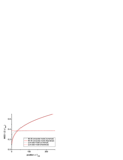
Figure 1: (Color online) The running diffusion coefficients $\left<\left(\Delta x(z)\right)^{2}\right>/(2zl_{slab})$ as a function of $z/l_{slab}$ are depicted. The analytical result (solid line) is compared to the numerical result (dashed line) for 20 % slab / 80 % 2D composite geometry. The analytical slab result (dash-dotted line) and the numerical slab result (dotted line) are also provided, for reference. The analytical and numerical results are are obviously in good agreement.

The numerical results are compared with the analytical results (presented above) in Fig. 1, by depicting the running diffusion coefficients $<\left(\Delta x(z)\right)^{2}>/(2zl_{slab})$ as a function of $z/l_{slab}$. An excellent agreement is witnessed among the theoretical and the numerical results, in both cases. The analytical expression (22) derived above for the asymptotic behavior of the field-line MSD thus appears to be valid in the composite turbulence model also and, in fact, bears a contributions which soon exceeds the diffusive result of the slab-model significantly: cf. the upper curve(s) in Fig. 1 to the lower, constant curve(s).

IV Further results and limits

We shall complete our study by considering various limiting cases, in which previous theoretical results are recovered. Although these results are not new, it is interesting per se to demonstrate that they can be obtained as appropriate limits from Eqs. (7-9).

IV.1 The initial free streaming regime

For small values of the position variable ($z\rightarrow 0$) hence expecting $\left<(\Delta x)^{2}\right>\rightarrow 0$, we obtain from Eq. (9)

$${d^{2}\over dz^{2}}\left<\left(\Delta x\right)^{2}\right>\approx{2\over B_{0}^{2}}\int d^{3}k\;P_{xx}(\vec{k})=2{\delta B_{x}^{2}\over B_{0}^{2}}.$$ (23)

Assuming vanishing conditions for both the MSD and its derivative at zero, one obtains

$$\left<\left(\Delta x\right)^{2}\right>={\delta B_{x}^{2}\over B_{0}^{2}}z^{2}$$ (24)

so a strong superdiffusive FL wandering regime is clearly found for small $z$, independent of the turbulence model adopted. For pure slab geometry it can easily be demonstrated that the initial free streaming solution is valid for $\mid z\mid\ll l_{slab}$. This means that Eq. (24) is valid for length scales which correspond to the inertial range of the turbulence wave spectrum.

IV.2 Quasilinear theory for field-line random walk

Within QLT, one may replace the MSD on the right hand side of Eq. (9) by the unperturbed field-lines (thus taking $\left<(\Delta x)^{2}\right>=0$), which yields

$${d^{2}\over dz^{2}}\left<\left(\Delta x\right)^{2}\right>={2\over B_{0}^{2}}\int d^{3}k\;P_{xx}(\vec{k})\cos(k_{\parallel}z).$$ (25)

QLT is thus apparently only exact for pure-slab turbulence, where $P_{lm}\sim\delta(k_{\perp})$; cf. Eq. (10). On the other hand, within QLT one finds for pure 2D and slab/2D composite turbulence [adopting Eqs. (15) and (25)] that $\left<(\Delta x)^{2}\right>=(\delta B_{x}/B_{0})^{2}z^{2}$, in disagreement with the nonlinear result obtained above. Thus, QLT fails to describe field-line wandering in the two-component model. Presumably, quasilinear theory might thus also not apply in other non-slab models.

IV.3 The diffusion limit

Combining Eq. (8) with the assumption of diffusion for the magnetic field-lines (i.e. explicitly setting $\left<(\Delta x)^{2}\right>=2\kappa\mid z\mid$) one obtains

$$\kappa={1\over B_{0}^{2}}\int d^{3}k\;P_{xx}(\vec{k})\int_{0}^{\infty}dz\;\cos(k_{\parallel}z)e^{-\kappa zk_{\perp}^{2}}.$$ (26)

The $z-$integral can easily be solved to give

$$\kappa={1\over B_{0}^{2}}\int d^{3}k\;P_{xx}(\vec{k}){\kappa k_{\perp}^{2}\over k_{\parallel}^{2}+(\kappa k_{\perp}^{2})^{2}}.$$ (27)

This formula is correct if field-line random walk behaves diffusively and if the small length scales of the initial free streaming regime are unimportant.

For two-component turbulence Eq. (27) can easily be evaluated; we find

$$\kappa=\kappa_{slab}+{\kappa_{2D}^{2}\over\kappa}\,,$$ (28)

using the slab diffusion coefficient $\kappa_{slab}$ of Eq. (14) and

$$\kappa_{2D}^{2}={1\over B_{0}^{2}}\int d^{3}k\;k_{\perp}^{-2}P_{xx}^{2D}(\vec{k})\,.$$ (29)

Eq. (28) is a quadratic equation in $\kappa$, which may easily be solved to get

$$\kappa={\kappa_{slab}+\sqrt{\kappa_{slab}^{2}+4\kappa_{2D}^{2}}\over 2}\,.$$ (30)

We note that this coincides with the result derived earlier by Matthaeus et al. mat95 . For pure slab turbulence, we have $\kappa_{2D}=0$, so the expected limit $\kappa=\kappa_{slab}$ is recovered. On the other hand, for pure 2D geometry, i.e. for $\kappa_{slab}=0$, one finds $\kappa=\kappa_{2D}$. Thus the parameter $\kappa_{2D}$ can be identified with the “diffusion coefficient” for pure 2D turbulence. However, adopting the standard spectrum of Eq. (21), one clearly obtains a diverging result:

$$\kappa_{2D}^{2} = 2C(\nu)l_{2D}{\delta B_{2D}^{2}\over B_{0}^{2}}\int_{0}^{\infty}dk_{\perp}k_{\perp}^{-2}\left(1+l_{2D}^{2}k_{\perp}^{2}\right)^{-\nu}$$ (31)

$$\rightarrow \infty.$$

The only possibility to prevent this singularity is the introduction of a finite box-size $L_{2D}\gg l_{2D}$ of the 2D fluctuations. Then we find

$$\kappa_{2D}^{2} = 2C(\nu)l_{2D}{\delta B_{2D}^{2}\over B_{0}^{2}}\int_{L_{2D}^{-1}}^{\infty}dk_{\perp}k_{\perp}^{-2}\left(1+l_{2D}^{2}k_{\perp}^{2}\right)^{-\nu}$$ (32)

$$= 2C(\nu){\delta B_{2D}^{2}\over B_{0}^{2}}\left({L_{2D}\over l_{2D}}\right)^{1+2\nu}{1\over 2\nu+1}\,\,l_{2D}^{2}$$

$$\times \;{}_{2}F_{1}\left(\nu,\nu+{1\over 2},\nu+{3\over 2};-{L^{2}\over l_{2D}^{2}}\right)\,,$$

where the integral was solved by applying exact relations which can be found in Ref. Grad . Because of $L_{2D}\gg l_{2D}$ we consider the asymptotic limit of the hypergeometric function ${}_{2}F_{1}(a,b;x)$ (see stegun ) to find for $\kappa_{2D}$ the expression

$$\kappa_{2D}=\sqrt{2C(\nu)\over 2\nu+1}\sqrt{l_{2D}L_{2D}}{\delta B_{2D}\over B_{0}}.$$ (33)

Within the diffusion theory for FLRW, the diffusion coefficient is strongly controlled by the box-size $L_{2D}$. In the light of the results presented in section III., the true reason for the divergent behavior (see Eq. (31)) may be the superdiffusive nature of field-line random walk. It appears that Eqs. (30) and (33) fail to provide an appropriate description of the composite turbulence, in contrast with the generalized nonlinear theory presented in this paper.

V Is a superdiffusive behaviour of FLRW reasonable?

A key result of the current article is the superdiffusive behaviour of FLRW for the slab/2D composite turbulence model (see Eq. (22) and Fig. 1). However, this nondiffusive result is clearly in disagreement with the assumption of diffusive field line wandering employed in several previous articles (see e.g. mat95 ).

The superdiffusive result derived here is based on two ad hoc assumptions which cannot be deduced from first principles:

1. A random phase (or Corrsin type) approximation was applied (see Eq. (4)).

2. A Gaussian distribution of field lines was assumed (see Eq. (9)).

Eq. (22) therefore provides an accurate result, suggesting a superdiffusive behavior of FLRW in real systems, provided that the latter two assumptions hold. However, one might draw the conclusion that the non-diffusivity deduced in this article is a consequence of (two) inaccurate approximations. We shall attempt to remove this ambiguity in the discussion that follows.

In another article (ShaKo07b ) we show that already for pure slab fluctuations where FLRW can be described without any assumptions or approximations, a superdiffusive result can be obtained be replacing the standard spectrum of Eq. (11) by a decreasing spectrum in the energy range. According to these results, superdiffusion indeed arises as the normal, by default behavior of FLRW. Classical (Markovian) diffusion can only be obtained in very special limits (wave spectrum exactly constant in the energy range and pure slab geometry).

The slab correlation function decays rapidly with increasing distance (see Eq. (18)). For decreasing wave spectra in the energy range and for non-slab models, however, we find a much weaker (non-exponential) decrease of the magnetic correlation functions. This weaker descrease of magnetic correlation functions provides a physical explanation of the nondiffusivity discovered in the current article.

A useful application but also a test of the superdiffusive result is cosmic ray scattering perpendicular to the mean magnetic field. In ShaKo07a the superdiffusive result obtained here is combined with a compound transport model based on the assumption that the guiding centers of the charged cosmic rays follow the magnetic field lines. In this article a quite good agreement between test particle simulations and the combination of compound transport and superdiffusion of FLRW was found. This agreement can also be seen as a proof of the validity of the two assumption (Corrsin’s hypothesis, Gaussian statistics) used in this article to deduce the superdiffusive result.

Furthermore, it is argued in ShaKo07a that for a diffusive behaviour of field line wandering one always obtains a strong subdiffusive behaviour of cosmic ray perpendicular scattering which cannot be true. Thus, the superdiffusive result deduced in the current article is not only a result obtained under certain assumptions. It seems that the real field lines indeed behave superdiffusively and that this superdiffusivity is essential for understanding charged particle propation.

From a purely fundamental point of view, the statistical-mechanical description of FLRW in magnetized plasmas bears certain generic physical characteristics which are encountered in various physical contexts. Our analytical findings are qualitatively reminiscent of earlier results by Isichenko on advection-diffusion problems Isio92 . Physically speaking, diffusive behavior of turbulence implies a fast decay of Lagrangian correlations, sufficiently fast for the limit $<(\Delta x)^{2}>/2t$ to converge. In fluid (non-plasma) environments, long scale random velocity fluctuations (depending on boundary conditions) may dominate the motion of a fluid element and may thus cause the limit to diverge. On the other hand, turbulent magnetized plasma systems are characterized by a plethora of nonlinear mechanisms, intertwined with the complex FL topology, which may add up in such a way that anomalous (non-classical) diffusion become the rule in plasmas. Persisting correlations among successive FL displacements are thus built-up, resulting in the superdiffusive behavior exposed in our work. This seems to suggest a general tendency of turbulent magnetized systems, so that previous diffusive FLRW considerations (obtained under various assumptions) should rather be treated with some caution.

It may be added that a superdiffusive result for FLRW was also obtained in various previous works, where distinct methodologies were employed. In Ref. Jo73 , the FL separation across the field was studied by adopting an ad hoc form for the magnetic correlation tensor; its behavior was found to be very sensitive to the exact form of the power spectrum, while a parabolic (ballistic) regime was shown to rule for steep spectra. In Ref. Skill74 , geometric (non-statistical) arguments were employed to study FLRW in galactic cosmic rays. A superdiffusive behavior was also found, independently from the turbulence spectrum (though mainly shallow spectra were considered therein). Similar findings were reported in Ref. Nar01 , in the context of thermal conduction in galactic clusters. A chaotic magnetic FL behavior (explicitly assumed to obey a Lyapunov behavior over a wide range of length scales), i.e. assuming an exponential FL divergence, was there shown to enhance perpendicular thermal conduction significantly, essentially increasing thermal conductivity in the transverse direction (previously thought to be much weaker than the parallel one) by a factor (up to) 5, as compared to the Spitzer value Spitzer . Still in the galactic thermal conduction context, Refs. Chan04 ; Maron04 have adopted a double diffusion concept, where particle diffusion along the field was related to FLRW in space, in order to study thermal conduction and electron diffusion along the magnetic field; a combined phenomenological, Fokker-Planck and numerical approach, FL displacement was shown to increase fast over length scales which are a multiple of the characteristic turbulence scale. Also note Ref. Matt03 (and the exhaustive discussion therein) for a nonlinear treatment of the perpendicular diffusion of charged particles (not FLRW).

VI Conclusion

A generalized nonlinear formulation has been presented, to describe field-line wandering (random walk) in general magnetostatic systems consisting of a statistical (or turbulent) component $\delta B$ and a nonstatistical uniform component $B_{0}$. Assuming vanishing parallel component of the turbulent field ($\delta B_{z}=0$), applying the Corrsin approximation, and assuming Gaussian statistics, a general ODE was deduced for the field-line MSD (Eq. (9)) in axisymmetric and homogeneous turbulent plasmas.

Adopting the two-component turbulence model which was suggested by Bieber et al. (bie96 ) as a realistic model for solar wind turbulence, it was demonstrated systematically that FLRW behaves superdiffusively. Specifically, a weakly superdiffusive behavior of the mean square deviation was found in the form $<(\Delta x)^{2}>\sim\mid z\mid^{4/3}$. This result was compared to previous results obtained via different assumptions, namely the quasilinear result ($<(\Delta x)^{2}>\sim z^{2}$) and the diffusive result $<(\Delta x)^{2}>\sim\mid z\mid$ of Ref. mat95 .

Extending the considerations in this article, the generalized nonlinear formulation presented here may be applied in a description of non-axisymmetric turbulence and/or other (e.g., anisotropic) turbulence geometries.

Since field-line random walk is of major importance in the description transport of charged particles in astrophysical plasmas, these results are significant in cosmic ray space physics and astrophysics. Concluding, the analytical expression(s) derived in this article provide a useful toolbox, which extends existing transport theoretical models and might be essential in inspiring forthcoming ones.

- (1) W.D. Mc Comb, The physics of fluid turbulence (Oxford Science Publications, UK, 1990).
- (2) R. Schlickeiser, Cosmic Ray Astrophysics (Springer, Berlin, 2002).
- (3) P. Goldreich, S. Sridhar, Astrophys. J., 438, 763 (1995).
- (4) J. Cho, A. Lazarian, E. T. Vishniac, Astrophys. J., 564, 291 (2002).
- (5) Y. Zhou, W. H. Matthaeus, P. Dmitruk, Rev. Mod. Phys., 76, 1015 (2004).
- (6) J. R. Jokipii, Astrophys. J., 183, 1029 (1973).
- (7) J. Skilling, I. McIvor, J. Holmes, MNRAS, 167, 87P (1974).
- (8) R. Narayan, R. Medvedev, M. Medvedev, 562, L129 (2001).
- (9) W. H. Matthaeus, G. Qin, J. W. Bieber, G. P. Zank, Astrophys. J., 590, L53 (2003).
- (10) B. Chandran, J. Maron, Astrophys. J., 602, 170 (2004).
- (11) J. Maron, B. Chandran, E. Blackman, PRL, 92, 045001 (2004).
- (12) J. Kóta, J. R. Jokipii, ApJ, 531, 1067 (2000).
- (13) G. M. Webb, G. P. Zank, E. Kh. Kaghashvili, J. A. le Roux, Astrophys. J., 651, 211 (2006).
- (14) J. R. Jokipii, Astrophys. J., 146, 480 (1966).
- (15) W. H. Matthaeus, P. C. Gray, D. H. Jr. Pontius, J. W. Bieber, Phys. Rev. Lett., 75, 2136 (1995).
- (16) S. Corrsin, Progress report on some turbulent diffusion research, in Atmospheric Diffusion and Air Pollution, in Atmospheric Diffusion and Air Pollution, Advanced in Geophysics, Vol. 6 (Eds. F. Frenkiel & P. Sheppard, Elsevier, New York, 1959), p. 161.
- (17) J. W. Bieber, W. Wanner, W. H. Matthaeus, J. Geophys. Res., 101, 2511 (1996).
- (18) A. Shalchi, I. Kourakis, Astronomy and Astrophysics, 470, 405 (2007).
- (19) I. S. Gradshteyn, I. M. Ryzhik, Table of integrals, series, and products, (Academic Press, New York, 2000).
- (20) M. Abramowitz, I. A. Stegun, Handbook of Mathematical Functions, (Dover Publications, New York, 1974).
- (21) A. Shalchi, I. Kourakis, Random walk of magnetic field lines for different values of the energy range spectral index, submitted to Physica Scripta.
- (22) M. B. Isichenko, Rev. Mod. Phys. 64, 961 - 1043 (1992).
- (23) L. Spitzer, Physics of Fully Ionized Gases (2nd Ed.; New York, Interscience, 1962).