The Distance to the Isolated Neutron Star RX J0720.4$-$3125

Abstract

We have used a set of dedicated astrometric data from the Hubble Space Telescope to measure the parallax and proper motion of the nearby neutron star RX J0720.4$-$3125. At each of eight epochs over two years, we used the High Resolution Camera of the Advanced Camera for Surveys to measure the position of the $B=26.6$ target to a precision of $\sim\!2$ mas ($\sim\!0.07$ pix) relative to 22 other stars. From these data we measure a parallax of $\pi=2.8\pm 0.9$ mas (for a distance of $360^{+170}_{-90}$ pc) and a proper motion of $\mu=107.8\pm 1.2\mbox{ mas yr}^{-1}$. Exhaustive testing of every stage of our analysis suggests that it is robust, with a maximum systematic uncertainty on the parallax of 0.4 mas. The distance is compatible with earlier estimates made from scaling the optical emission of RX J0720.4$-$3125 relative to the even closer neutron star RX J1856.5$-$3754. The distance and proper motion imply a transverse velocity of $180^{+90}_{-40}\mbox{ km s}^{-1}$, comparable to velocities observed for radio pulsars. The speed and direction suggest an origin for RX J0720.4$-$3125 in the Trumpler 10 OB association $\sim\!0.7$ Myr ago, with a possible range of 0.5–1.0 Myr given by the uncertainty in the distance.

1. Introduction

One of the many interesting results from ROSAT All-Sky Survey (Voges et al., 1999) was the discovery of seven objects that appear to be nearby, thermally-emitting neutron stars that have little if any magnetospheric emission (for recent reviews, see Haberl 2004, 2006; van Kerkwijk & Kaplan 2006). These objects, known most commonly as “isolated neutron stars,” (INS) are distinguished by their long spin periods ($\gtrsim\!3$ s, when measured), largely thermal spectra with cool temperatures ($kT\lesssim 100$ eV), faint optical counterparts, and lack of radio emission.

Thermally-emitting neutron stars have been the targets of many observations, as they can potentially be used to constrain the equation of state (EOS) of neutron stars, and thereby explore nuclear physics in realms inaccessible from laboratories (e.g., Lattimer & Prakash, 2000). Two main approaches are used. The first, using the spectrum, seems simple: determine the effective angular size from spectral fits, multiply by the distance (obtained by other means), and one has the apparent radius. This radius can be converted into the physical radius through use of mass. The radius is the crucial quantity in differentiating between EOS, as most EOS predict a distinctive but small range of radii for a large range of masses. The second method is to use measurements of an ensemble of neutron stars to constrain cooling curves, which are themselves sensitive to the EOS and the interior composition (for a review, Yakovlev & Pethick, 2004). This also seems simple: measure the received flux of an object, convert to a luminosity using the distance, and with the age place that object on a cooling diagram. The closest of the INS, RX J1856.5$-$3754 (catalog RX J1856.5-3754), has been the subject of much inquiry for just these purposes (e.g., Walter & Lattimer, 2002; Drake et al., 2002; Braje & Romani, 2002).

Table 1HST ACS/HRC F475W Observation Summary

	Date		Orientation	$m_{475}$
Epoch	(UT)	(MJD)	(deg)	(mag)
1	2002 Jul 04	52460.0	353.0108	26.66
2	2002 Sep 15	52532.6	072.5457	26.54
3	2003 Jan 06	52645.1	175.9862	26.45
4	2003 Mar 16	52714.0	254.8005	26.57
5	2003 Aug 04	52855.1	028.0808	26.39
6	2003 Sep 21	52903.0	077.1792	26.45
7	2004 Jan 07	53011.9	178.4808	26.42
8	2004 Mar 19	53083.1	258.1951	26.64

Note. — For each epoch, eight exposures were taken during two orbits. For epochs 1–4, the integration times for exposures 1–4 were 600 s, while those for exposures 5–8 were 630 s. For epochs 5–8, the exposure times were 625 s in the first orbit, and 660 s in the second. The dither offsets along the $x$ and $y$ axes of the detector (written in base eight, where, e.g., 2.2 is $2+\frac{2}{8}$), were [0.0, 0.0], [2.2, 2.2], [4.4, 4.4], [6.6, 6.6], [1.1, 5.5], [3.3, 7.7], [5.5, 1.1], and [7.7, 3.3]).

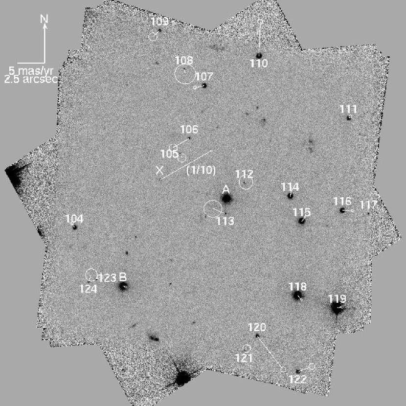
Figure 1.— Combined image of all 64 HRC exposures of the field of RX J0720.4$-$3125 (made using multidrizzle; Koekemoer et al. 2002). The objects used for the astrometry are labeled (remaining objects were either too faint or too extended to be used). We also show the fitted proper motions of those objects, with the ellipses indicating the 1$\sigma$ uncertainties on the proper motion. Note that the proper motion of RX J0720.4$-$3125 (object “X”) has been scaled down by a factor of $1/10$ compared to the other objects in the field. The scales and orientation are indicated in the upper left corner.

While the basic approaches — inferring radii from broad-band spectral fits and comparing cooling luminosities to models — are easily stated, complications arise from uncertainties in distances and ages; additional complications may result from the presence of strong surface magnetic fields and unknown surface compositions. Progress on these last issues has been made recently from X-ray spectroscopy (Haberl et al., 2003; van Kerkwijk et al., 2004; Haberl et al., 2004b; Zane et al., 2005) and timing (Kaplan & van Kerkwijk, 2005a, b), but distances and ages are difficult to measure. The technique necessary for both is high-precision optical astrometry, as shown by the example of RX J1856.5$-$3754: with a series of Hubble Space Telescope (HST) observations it was possible to measure the parallax (Kaplan, van Kerkwijk, & Anderson 2002b, hereafter KvKA02; Walter & Lattimer 2002), and the proper motion traced the object to an OB association where it was likely born (Walter, 2001).

While RX J1856.5$-$3754 is the brightest and closest of the INS, and has thus garnered most of the attention, it is best to try to use multiple sources. This especially since each source appears to have peculiarities, be it stronger or weaker timing noise, stronger or weaker features in the X-ray spectra, presence or absence of long-term variations, or the presence of an H$\alpha$ nebulae (in the case of RX J1856.5$-$3754; van Kerkwijk & Kulkarni 2001). Likely, secure results will only be obtained if we understand and can correct for these differences. Here, we discuss high-precision astrometric observations of the second brightest source, RX J0720.4$-$3125 (catalog RX J0720.4-3125).

RX J0720.4$-$3125 was discovered by Haberl et al. (1997) as a soft ($kT\simeq 80$ eV), bright X-ray source in the ROSAT All-Sky Survey. Given its low hydrogen column density ($N_{H}\sim 1\times 10^{20}\mbox{~{}cm}^{-2}$), nearly sinusoidal 8.39-s pulsations, relatively constant X-ray flux, and faint ($B=26.6$ mag), blue optical counterpart (Kulkarni & van Kerkwijk, 1998; Motch & Haberl, 1998), it was classified as a nearby, isolated, thermally-emitting neutron star. X-ray timing observations (Kaplan & van Kerkwijk, 2005a) give a characteristic age of 2 Myr and a magnetic field strength of $2.4\times 10^{13}$ G, consistent with suggestions of the source being an off-beam, moderately strong-field radio pulsar (Zane et al., 2002; Kaplan et al., 2002a). While the above properties make RX J0720.4$-$3125 a prototypical INS, X-ray monitoring over the last few years has uncovered unique behavior: the X-ray spectrum and pulse shape have been evolving (de Vries et al., 2004; Vink et al., 2004). This may indicate free precession (Haberl et al., 2006), although this interpretation is not unique (van Kerkwijk & Kaplan, 2006). Scaling to RX J1856.5$-$3754, its distance was estimated to be $\sim\!300$ pc (KvKA02). Motch et al. (2005) measured a proper motion of $97\pm 12\mbox{ mas yr}^{-1}$ from ground-based astrometry, and suggested the source might originate in the OB association Trumpler 10, something we independently derived from part of the data presented here (Kaplan, 2004).

In this paper, we present a detailed analysis of HST observations of RX J0720.4$-$3125 specifically designed for astrometry, which we use to measure its proper motion and parallax. The organization of this paper is as follows. First, in § 2, we present the astrometric observations and discuss additional observations we used for photometry and for tying our astrometry to the International Coordinate Reference System (ICRS). We also discuss the basic reduction of these data. Then, in § 3, we use the photometry to determine photometric parallaxes of the reference stars, which we use in § 4 for the parallax. We discuss the implications in § 5 and conclude in § 6.

Our analysis is complex and necessarily involves choices among alternate schemes. Previous attempts to measure parallaxes with HST made choices that were later called into question (Walter 2001; KvKA02; Walter & Lattimer 2002). To clarify our analysis, and to set out the framework for future work, we give full details on the parallax measurement in App. A. We then show that our results are robust to the choices we made by describing various alternate analyses in App. B. In what follows, we define our proper motions in Right Ascension and Declination $(\mu_{\alpha},\mu_{\delta})$ such that the scales are the same and no $\cos\delta$ term is necessary. All uncertainties are $1\sigma$ unless otherwise indicated. In addition to the results presented in Tables 4–6, we make the raw data available electronically.

2. Observations, Reduction, and Analysis

Our main data set consist of 64 exposures taken during eight visits of the field of RX J0720.4$-$3125 with HST; a summary is given in Table 1. All data were taken with the High Resolution Camera (HRC, with a plate-scale of $28.27{\rm~{}mas\,pix}^{-1}$) and the F475W (SDSS $g^{\prime}$) filter, which has good sensitivity to the blue colors of RX J0720.4$-$3125.

We tried to optimize our observations for measuring an accurate parallax in three ways. First, we observed over two years, to minimize the covariance between proper motion and parallax, and verify repeatability. Second, we observed four times per year rather than just at the parallactic maxima, to reduce possible systematic effects of observing at orientations different by 180° only. Third, for the eight exposures in each epoch, we chose dither positions optimized for sampling fractional pixel phase.

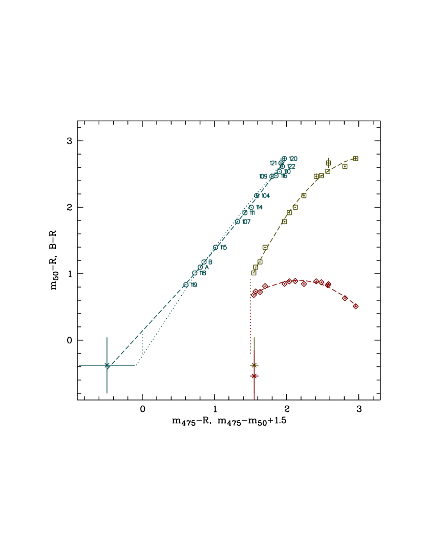
Figure 2.— Color-color relations used to infer $B-R$ and $R$ for stars for which the ground-based photometry was inaccurate. Shown are relations between $B-R$ and $m_{475}-R$ (circles), $B-R$ and $m_{475}-m_{50}$ (squares), and $m_{50}-R$ and $m_{475}-m_{50}$ (lozenges), with the $m_{475}-m_{50}$ magnitudes offset by 1.5 mag for clarity; the zero points are indicated vertical dotted lines. Overdrawn (long-dashed lines) are the empirical quadratic fits from Table 3 to all points except RX J0720.4$-$3125 (crossed points), as well as the relation between $B-R$ and $m_{475}-R$ expected from synthetic photometry (dotted line; Sirianni et al. 2005).

In our analysis, we also use three sets of observations presented previously. For photometry, these are B- and R-band images taken with the Low Resolution Imaging Spectrometer (LRIS) on Keck (Kulkarni & van Kerkwijk, 1998), and images taken with the Space Telescope Imaging Spectrograph (STIS) on HST (Kaplan et al., 2003), and for our astrometric tie, B-band observations taking with the Focal Reducer, low-dispersion Spectrograph (FORS1) on the Very Large Telescope (Motch, Zavlin, & Haberl, 2003).

Below, we describe first the reduction of all data sets, and then the way we measured positions from the HRC images, tied our astrometry to the International Celestial Reference System, and obtained photometry from the HRC, STIS and LRIS data. For reference, we show a combined image of all HRC data in Fig. 1, with stars used in our analysis labeled.

2.1. Reduction

For each data set, the basic reduction was standard: bias and dark current were subtracted, and possible pixel-to-pixel sensitivity variations were corrected for using flat fields. For the HST data, these steps are taken in the standard pipelines, while for the LRIS data they were performed by Kulkarni & van Kerkwijk (1998). For the FORS images, which we retrieved from the archive and re-analyzed, we determined the bias level from the overscan regions and constructed a flat field from dawn sky images.

Table 2Photometry and photometric parallaxes for stars in the field of RX J0720.4$-$3125

	Observed				Inferred
	$B$	$m_{475}$	$m_{50}$	$R$	$R_{\rm ad}$	$({\it B},{\it R})_{\rm ad}$		$M_{R,\rm MS}$	$\pi_{\rm phot}$
ID	(mag)	(mag)	(mag)	(mag)	(mag)	(mag)	Source	(mag)	(mas)
X	26.62(17)	26.51(4)	26.45(5)	27.0(4)	27.0(4)	$-$0.4(4)	B,R	$\cdots$	$\cdots$
A	20.517(4)	20.221(5)	20.150(10)	19.418(3)	19.418(3)	1.099(5)	B,R	4.5	0.105
B	20.789(4)	20.468(5)	20.337(10)	19.612(3)	19.612(3)	1.177(5)	B,R	4.8	0.110
104	23.60(2)	23.012(5)	22.272(11)	21.425(15)	21.425(15)	2.17(3)	B,R	7.5	0.166
105	27.0(2)	25.801(18)	24.578(15)	23.84(2)	23.84(2)	2.68(5)	475,R	9.5	0.134
106	26.47(13)	25.653(18)	24.391(14)	23.66(2)	23.66(2)	2.73(5)	475,R	9.7	0.165
107	23.384(9)	22.920(6)	22.448(11)	21.600(4)	21.600(4)	1.784(10)	B,R	6.6	0.101
108	$\cdots$	26.77(4)	25.50(2)	24.98(8)	24.82(9)	2.67(8)	475,50	9.4	0.082
109	25.08(4)	24.410(12)	23.499(12)	22.613(7)	22.613(7)	2.44(3)	475,R	8.3	0.140
110	22.735(5)	22.094(3)	21.022(10)	20.195(3)	20.195(3)	2.540(6)	B,R	8.7	0.51
111	23.731(12)	23.235(8)	22.698(11)	21.813(4)	21.813(4)	1.918(12)	B,R	6.9	0.105
112	$\cdots$	26.43(3)	25.127(20)	24.4(2)	24.47(7)	2.69(7)	475,50	9.5	0.102
113	$\cdots$	26.79(4)	25.60(3)	$\cdots$	24.86(9)	2.62(9)	475,50	9.1	0.072
114	22.514(6)	22.024(5)	21.404(10)	20.514(3)	20.514(3)	2.000(6)	B,R	7.1	0.21
115	21.774(4)	21.392(6)	21.190(10)	20.377(3)	20.377(3)	1.398(5)	B,R	5.6	0.111
116	23.045(8)	22.422(8)	21.441(10)	20.569(4)	20.569(4)	2.476(9)	B,R	8.5	0.38
117	27.1(3)	26.43(3)	25.30(2)	24.48(6)	24.53(7)	2.59(7)	475,50	9.0	0.077
118	20.510(4)	20.225(5)	20.179(10)	19.498(3)	19.498(3)	1.012(5)	B,R	4.2	0.087
119	19.689(3)	19.461(7)	$\cdots$	18.855(3)	18.855(3)	0.834(4)	B,R	3.5	0.087
120	24.73(3)	23.965(11)	22.507(11)	21.997(8)	21.997(8)	2.73(3)	B,R	9.8	0.36
121	25.86(7)	25.115(17)	24.036(13)	23.193(15)	23.193(15)	2.62(4)	475,R	9.1	0.154
122	24.135(16)	23.459(5)	22.151(11)	21.519(6)	21.519(6)	2.616(17)	B,R	9.1	0.33
123	25.92(16)	25.229(14)	23.861(12)	23.22(3)	23.25(5)	2.71(5)	475,50	9.7	0.191
124	27.3(3)	26.304(20)	24.759(16)	24.56(7)	24.31(6)	2.75(6)	475,50	9.9	0.132

Note. — Observed: All errors quoted exclude the zero-point uncertainties to which the measurements are on the Vega system. These are $\lesssim\!0.02~{}$mag for all but $m_{50}$, which is only roughly calibrated (see §2.4). Reasons for missing measurements are: 108 and 112 ($B$): too faint; 113 ($B$ and $R$): too close to star A; 119 ($m_{50}$): overexposed. Inferred: $R_{\rm ad}$ and $({\it B},{\it R})_{\rm ad}$ are our adapted values, inferred from the magnitudes listed under Source. The inferred absolute magnitudes $M_{R,\rm MS}$ have uncertainties around 0.4 mag, and the corresponding uncertainties in the photometric parallaxes $\pi_{\rm phot}$ are about 20% (see §3).

Table 3Color transformations used to infer $B-R$ and $R$ for stars in the field.

					rms
Color		Empirical Relation			(mag)
$B-R$	$=$	$+0.116$	$+1.173\,(m_{475}-R)$	$+0.067\,(m_{475}-R)^{2}$	$+0.030$
$B-R$	$=$	$+0.915$	$+2.270\,(m_{475}-m_{50})$	$-0.700\,(m_{475}-m_{50})^{2}$	$+0.049$
$m_{50}-R$	$=$	$+0.654$	$+0.759\,(m_{475}-m_{50})$	$-0.579\,(m_{475}-m_{50})^{2}$	$+0.028$

In preparation for further analysis, we flagged bad pixels and made averages. For the HRC data, we used a procedure similar to that of multidrizzle (Koekemoer et al., 2002), but which does not correct for distortion. First, we removed pixels flagged as bad in the data quality array, as well as two obvious bad columns [upwards from pixel $(x,y)=(200,548)$ and $(617,228)$]. Next, we subtracted the sky level and resampled on an eight times finer grid, for which the dither positions correspond to integer pixel offsets. Using these offsets, we registered the images for each epoch and constructed an initial guess at a cosmic-ray free, average image from the two lowest values at each position.

For each image, we flagged as cosmic-ray hits all pixels in excess by more than $5\sigma$ of those in the initial average (resampled back to the original resolution) as well as all adjacent pixels. Here, we estimated $\sigma$ by adding, in quadrature, the read-out noise, the Poisson noise due to sky and signal (as inferred from the average), as well as terms equal to 5% of the signal and 5% of the range in signal in the surrounding $3\times 3$ pixel box. The latter terms ensure centers of bright stars are not incorrectly flagged as bad due to registration errors, focus changes, etc. We also constructed a final average for each epoch from those cleaned images.

For the STIS data, the analysis was similar, except that no resampling was necessary, since integer pixel offsets were used. For the LRIS and FORS images, we used more standard methods to correct for cosmic-ray hits, in which they are identified by their narrow width compared to the seeing, and replaced by interpolation. For the photometry and astrometry below, averages were made of these filtered images, registered to integer pixel shifts.

2.2. Position Measurements

We determined positions using the “effective” point-spread function (ePSF) technique of Anderson & King (2000). We use the ePSF determined for the HRC with the F475W filter by Anderson & King (2004, hereafter AK04), and use a variation of their procedure for the fits. In App. B.1, we describe where we deviate and discuss further variations; fortunately, our results do not depend much on our choices, although the method described here gives slightly superior precision.

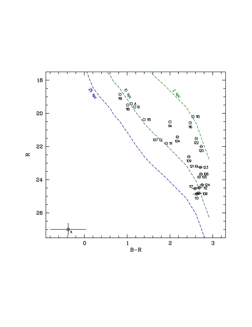
Figure 3.— Color-magnitude diagram, showing $R$ magnitude versus $B-R$ color for the objects in Table 2. We also show main sequences with reddening $A_{V}=0.25$ mag at 2, 8.5, and 25 kpc (as labeled). One sees that most stars are at about 10 kpc distance, implying that their photometric parallaxes are small, about 0.1 mas.

In our procedure, we fit stellar images on each exposure using the pixels in a radius of 2.56 pixels around an initial guess for the centroid (determined from a Gaussian fit in the average image), weighting data points with uncertainties $\sigma=(\textrm{RN}^{2}+\max(F,\textrm{sky})/\textrm{G})^{1/2}$ (where $\textrm{RN}=6$ DN is the read-noise, which we determined empirically from variations in background regions, and $\textrm{G}=1{\rm~{}e^{-}\,DN^{-1}}$ is the gain for pipe-line processed HRC images). We fit simultaneously for the position and amplitude of each star, but fix the sky to the header value mdrizsky, which is determined by the pipeline drizzle process (and is very similar to the median or mode of all pixel values). Finally, we correct the positions for distortion in the HRC using the solution from AK04.

To estimate uncertainties on the positions, we used the standard technique for $\chi^{2}$ fitting in which we determined the $x$ and $y$ offsets at which $\chi^{2}$ increased by 1. It is worth noting that, generally, this is only valid if the fit is acceptable, i.e., if $\chi^{2}$ roughly equals the number of degrees of freedom. For the brightest stars, we often find much larger $\chi^{2}$, since the PSF varies due to focus changes, etc. One could rescale the errors, but this would lead one to overestimate the uncertainties of positions of stars relative to each other (which is what enters our analysis), since PSF changes affect all stars in the same way. Therefore, we retained the formal uncertainties, verifying that they lead to acceptable fits (see below and App. B.2).

With positions and uncertainties in hand, we solve for the best-fit transformation between the first and the other seven exposures for each epoch (for details, see App. A), and determine one set of average, distortion-corrected positions per epoch. Given our weighting, the four brightest stars (A, B, 118, and 119) dominate the fits. For the transformation, we follow AK04 and use a 6-parameter, bi-linear transformation, as we do for the transformation between epochs (see § 4). This fits for a central position, the overall plate-scale and rotation of the image, and a second plate-scale and rotation that reflect differences in scale and orientation between the two axes (we test variations on this in App. B.4).

In general, when we included all measurements, the fit quality for some transformations was very poor. Inspecting the outliers, we found that within the fitted region of most there were some pixels flagged as bad. These pixels are not included in the ePSF fit, so to first order they should not affect the result. There is a second-order effect, however: that arises because our model ePSF is not a perfect match to the real one. As stated above, generally, this does not matter for relative positions, since the ePSF is wrong in the same way for all stars. But this relies on the same part of the ePSF being used, which is not possible if bad pixels are present. Because of this, we decided to exclude all position measurements that had bad pixels. In addition, we excluded all measurements of star 114 in epoch 4, where it is close to the HRC occulting finger and clearly deviant, and three further significant outliers without obvious causes (star 115 in epoch 2, exposure 2; 118 in 3, 5; and A in 7, 7).

With the above exclusions, the fits are fairly good, with the overall $\chi^{2}_{\rm red}$ ranging from 1.00 for epoch 8 to 1.48 for epoch 5. Furthermore, all individual sources were found to fit well too (for details, including simulated data, see App. B.2 and Fig. 8).

2.3. Absolute Astrometry

While the HRC observations provide very accurate relative positions, the precision with which these can be tied to the International Celestial Reference System (ICRS) is not as good, as it is determined by the less accurately known positions of the guide stars used. To improve the precision, we use ground-based observations to tie our measurements to the UCAC2 catalog (Zacharias et al., 2004), which is currently the most precise representation of the ICRS for stars fainter than those measured by Hipparcos.

We first tied a short FORS image taken on 31 December 2002, which is very close in time to our third HRC observation, to the UCAC2 catalog (corrected to the same epoch using the UCAC2 proper motions). We measured centroids of 13 UCAC2 stars present on the image and corrected for radial distortion using the quadratic relation given by Jehin, O’Brien, & Szeifert (2006). A four-parameter transformation sufficed, with the offset accurate to 10 mas, and scale and rotation different from nominal by $-0.028\pm 0.012$% and $-0\fdg 076\pm 0\fdg 008$, respectively. The fit was good, with the residuals consistent with the UCAC2 uncertainties.

We then used 41 stars to transfer the tie to a deeper image, consisting of twenty 620-s images from 29, 30, and 31 December 2002. This fit was again good, and the uncertainties negligible compared to the first step. Finally, we tied our astrometry to the HRC using 18 stars for which we could obtain accurate FORS positions. Using HRC positions evaluated at the FORS epoch using the proper motions derived in §4, we find an excellent tie, with offsets accurate to $\sim\!2$ mas and a scale and position angle different from the nominal values by $-0.034\pm 0.015\%$ and $-0\fdg 018\pm 0\fdg 010$, respectively (here, the uncertainties take into account that the HRC shows deviations from equality of scales and orthogonality; see § 4).

The overall precision with which our measurements are on the UCAC2 system is limited by the first step, and is $\sim\!11$ mas, similar to the precision with which UCAC2 is on the ICRS (Zacharias et al., 2004). For the scale and position angle, the first and last step contribute; we estimate that the scale is accurate to 0.02% and the position angle to $0\fdg 011$.

Below, we will give positions relative to star A, fixing its position to $\alpha_{\rm J2000}=07^{\rm h}20^{\rm m}24\fs 4837$, $\delta_{\rm J2000}=-31^{\circ}25^{\prime}51\farcs 786$. We will also correct the nominal scale and position angles of epochs 3 and 7 using the values found above.

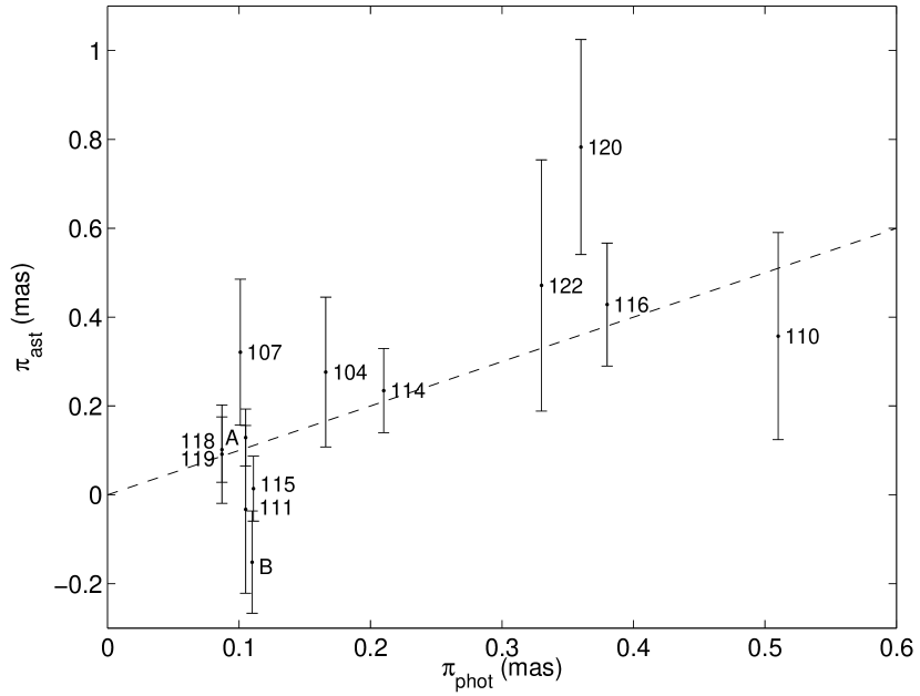
Figure 4.— Photometric versus astrometric parallaxes for the stars from Table 2 for which the astrometric measurement error was less than 0.3 mas; the dashed line indicates $\pi_{\rm ast}=\pi_{\rm phot}$. In measuring the astrometric parallaxes, we held all reference stars but the one labeled fixed at their photometric parallaxes, and then solved for the parallax of the reference star in question.

2.4. Photometry

For the HRC photometry, we measured fluxes in the averaged flat-fielded images for each epoch (see § 2.2). Since the HRC flux for RX J0720.4$-$3125 will help constrain the different components of the optical emission (Kaplan et al., 2003), we took care to correct for all known systematic effects, following the prescription of Sirianni et al. (2005) for flat-fielded, non-drizzled images. Briefly, we first measured counts in a range of apertures using DAOPHOT (Stetson, 1987), and sky in a 50 to 60 pixel annulus (1$\farcs$33–1$\farcs$59). We chose an aperture of 3 pixels radius (0$\farcs$08) as a compromise between adequate signal-to-noise ratio for fainter targets and minimal effects from PSF variations over the detector. Next, we corrected for pixel-area variations and charge transfer inefficiencies following Pavlovsky et al. (2006). We used brighter, isolated stars to determine the aperture correction to an 18-pixel (0$\farcs$48) aperture, and added a fixed $-0.103~{}$mag to correct to “nominal infinity” (Sirianni et al., 2005); the latter includes the small, $-0.003~{}$mag effect from contamination of the sky by starlight. Finally, we added the zero point of 25.623 to obtain magnitudes in the Vega system.

We checked for, but found no significant variations for any star (for star 113, we rejected epochs 1 and 3, since a trail from star A passed over the image). For RX J0720.4$-$3125, where we list the individual measurements in Table 1, the standard deviation is 0.10 mag, consistent with the error of 0.09 mag and with numbers for other faint sources (e.g., 0.09 and 0.10 mag for stars 112 and 108, respectively). We list the average magnitudes in Table 2.

For STIS, we again used DAOPHOT to measure fluxes, choosing a 2-pixel (0$\farcs$1) aperture. We corrected for charge transfer inefficiencies following Goudfrooij & Kimble (2002, see also ), and used brighter stars to correct to a 10 pixel (0$\farcs$5) radius aperture. To place our magnitudes roughly on the STScI system, we added an additional $-0.100~{}$mag to “nominal infinity,” and used the zero point flux of $0.9987\times 10^{-19}\mbox{ erg cm}^{-2}\mbox{ s}^{-1}\mbox{ \AA}^{-1}$ for a count rate of $1{\rm~{}s^{-1}}$, and the magnitude offset of 21.1, as described in the HST data handbook. We stress that while the results are fine for our purpose of inferring stellar colors (since calibration errors will be taken out), care has to be taken in interpreting them in terms of absolute fluxes. In particular, for the flux of RX J0720.4$-$3125 itself, see the detailed discussion in Kaplan et al. (2003).

For the LRIS photometry, Kulkarni & van Kerkwijk (1998) had found that scattered light from much brighter stars made photometry difficult, and they adopted a simplified PSF fitting technique. In order to measure not just isolated stars, but also ones near others, we modified their procedure slightly, using the positional information from the HRC and picking a moffat function instead of a Gaussian as a PSF model. The results, listed in Table 2, are consistent with those of Kulkarni & van Kerkwijk (1998). They are also roughly consistent (brighter by $\sim\!0.03~{}$mag) with those of Motch & Haberl (1998) and Motch et al. (2003).

3. Photometric parallaxes of background sources

In measuring the parallax of RX J0720.4$-$3125, we need to worry about bias by parallaxes of our background sources. Typical distances may range from 1 to 10 kpc, inducing an effect at the 1 to 0.1 mas level. Generally, one might expect more nearby sources to bias the fit most, since these would be brighter and hence have heavier weight. Given this, it is good to have distance estimates, which, even if wrong for individual sources, reduce any systematic bias. For this purpose, we use our photometry: we estimate temperature from $B-R$ and flux from $R$, and then infer a distance assuming the stars are on the main sequence.

For many stars, we have $B$ and $R$ magnitudes from our Keck images (§2.4). Some stars, however, were too faint (in particular in $B$) or too close to brighter stars for reliable photometry. For those, we infer $B-R$ and $R$ from the HRC and STIS photometry, using empirical color-color relations determined from stars with uncertainties in $B-R$ smaller than 0.1 mag; see Fig. 2 and Table 3. We find that all relations are tight, with root-mean-square residuals of less than 0.05 mag. Between $m_{475}-R$ and $B-R$, the relation is almost linear, while the relations between $m_{475}-m_{50}$ and $B-R$, and $m_{475}-m_{50}$ and $m_{50}-R$ are well-described by quadratic functions. By way of verification, we compared our result for $m_{475}-R$ and $B-R$ with the relation expected from synthetic photometry on model atmospheres (Sirianni et al., 2005). As can be seen in Fig. 2, the agreement is good.

We proceeded by estimating $B-R$ values from $m_{475}-R$ and $m_{475}-m_{50}$ for all stars; for a given star, we adopt the $B-R$ estimate with the smallest uncertainty (where the uncertainty includes in quadrature the measurement uncertainty and the scatter around the required transformation). For objects for which $B-R$ was inferred from $m_{475}-m_{50}$, we estimated $R$ from $m_{50}$ using the relation between $m_{475}-m_{50}$ and $m_{50}-R$.

In Fig. 3, we show our adopted $B-R$ and $R$ estimates in a color-magnitude diagram. Also shown are expected colors and magnitudes for main-sequence stars at various distances, for a reddening of $A_{V}=0.25$ (see below). For these, we used the absolute magnitudes $M_{V}$ and colors from Cox (2000; specifically, we obtained $M_{V}$ and $B-V$ from Table 15.7, and converted to $M_{R}$ and $B-R$ using Table 15.11; we cannot use Table 15.7 directly since our R-band magnitudes are in the Kron-Cousins system). One sees that if our objects are main-sequence stars, they lie between 2 and 20 kpc; the estimated photometric parallaxes are listed in Table 2. We note that it is very unlikely that they are not main-sequence stars: if they were giants, they would be well outside the Galaxy, while if they were white dwarfs, we would find a significant parallax.

The photometric parallaxes for the brighter stars, which carry most weight in our astrometry, are all around 0.1 mas, and thus even large fractional errors in these will not influence our conclusion much. Nevertheless, it is worth briefly considering the main sources of error. Likely, these are the assumed reddening and metallicity. For the reddening, we used $E_{B-V}=0.08$, derived by Motch & Haberl (1998) from UBV photometry of stars near RX J0720.4$-$3125. This is consistent with the $E_{B-V}\simeq 0.07$ inferred from the observed $B-R$ colors of stars A and B and their G2 and G5 spectral types (as inferred from the spectra of Haberl et al. 1997; see also Motch & Haberl 1998). It is somewhat lower than the total line-of-sight extinction $E_{B-V}=0.14$ estimated from background infrared emission (Schlegel, Finkbeiner, & Davis, 1998).

The above estimates assume solar metallicity. A sub-solar metallicity may be more likely, however, since the background sources are relatively high above the plane and at large Galactocentric radius: for $(\ell,b)=(244\fdg 16,-8\fdg 16)$ and at 10 kpc, one finds $z=1.4$ above the Galactic plane and Galactocentric radius $\varpi=16$ kpc, (we ignored that the plane is warped down by $\sim\!3^{\circ}$ at $\ell=240^{\circ}$; Momany et al. 2006). This may also influence the reddening: for ${\rm[Fe/H]}=-1.0$, Motch & Haberl (1998) infer a lower reddening $E_{B-V}=0.04$ from their UBV photometry, while from stars A and B one infers a higher reddening $E_{B-V}\simeq 0.14$ (since they would be intrinsically bluer).

To estimate the maximum effect of sub-solar metallicity, we combined the increased intrinsic blueness, decreased luminosity, and increased reddening for star A. We found that a change of 0.6 mag in distance modulus, or a factor 1.3 in photometric parallax. For stars of later spectral type, the effect is less. Since the brighter background stars are so distant, the additional uncertainty in the parallax of RX J0720.4$-$3125 should be less than 0.1 mas.

4. Measuring the Parallax

Our goal is to measure the proper motion and parallax of RX J0720.4$-$3125, but this has to be done relative to other stars, for which the positions, proper motions and parallaxes are not known a priori, and on images for which our knowledge of the positions, rotations, and scales is insufficiently accurate. In our procedure, we fit simultaneously for our target parameters and all other parameters. We have to fix some of those, however, since otherwise the fit is degenerate (e.g., a net shift between epochs cannot be distinguished from a proper motion component common to all stars). We made the following choices.

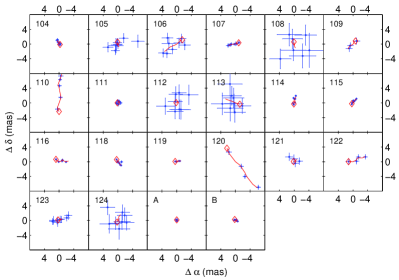
Figure 5.— Positions of the reference stars at every measured epoch, with the predicted track based on the best-fit proper motion and photometric parallax indicated by the solid line. The diamond indicates the fitted position at the epoch of the first observation.

Table 4Astrometry of Reference Sources

		$m_{\rm instr}$	$\Delta\alpha$	$\Delta\delta$	$\mu_{\alpha}$	$\mu_{\delta}$
ID	$N_{\rm epoch}$	(mag)	(arcsec)	(arcsec)	(mas yr-1)	(mas yr-1)	$\chi^{2}_{\rm red}$
X	8	$-5.7$	0+$6.1219(8)$	0+$1.7026(9)$	$-93.9(12)$	$52.8(13)$	1.13
A	8	$-12.0$	0+$0$	0+$0$	0+$0$	0+$0$	0.67
B	8	$-11.8$	0+$9.46094(12)$	$-8.01896(11)$	$-0.45(17)$	$-0.18(17)$	0.50
104	7	$-9.2$	$13.92144(16)$	$-2.65145(15)$	0+$0.4(2)$	0+$0.8(2)$	0.44
105	8	$-6.4$	0+$4.2079(5)$	0+$4.0488(5)$	$-0.2(7)$	$-0.7(7)$	1.83
106	8	$-6.5$	0+$3.4296(5)$	0+$5.5332(5)$	0+$2.9(7)$	$-1.8(7)$	0.93
107	8	$-9.3$	0+$2.03280(16)$	$10.34588(16)$	0+$1.7(3)$	$-0.3(3)$	0.51
108	7	$-5.4$	0+$3.8609(14)$	$11.8761(13)$	$-0.2(19)$	$-0.9(18)$	1.19
109	3	$-7.8$	0+$6.1437(5)$	$15.4211(5)$	0+$1.3(7)$	$-1.2(7)$	1.39
110	5	$-10.2$	$-2.9762(3)$	$13.0787(3)$	$-0.2(4)$	0+$6.3(4)$	0.53
111	7	$-9.0$	$-11.21837(18)$	0+$7.37302(18)$	$-0.3(3)$	0+$0.3(3)$	0.98
112	8	$-5.8$	$-1.6390(8)$	0+$1.4360(8)$	$-0.3(12)$	0+$0.2(13)$	0.96
113	8	$-5.5$	0+$0.1059(10)$	$-1.3660(9)$	0+$2.3(16)$	0+$0.9(15)$	0.46
114	7	$-10.2$	$-5.84398(9)$	0+$0.22906(9)$	$-0.25(14)$	0+$1.28(14)$	0.99
115	8	$-10.9$	$-6.88576(9)$	$-2.06279(8)$	$-0.69(13)$	0+$0.83(13)$	0.62
116	6	$-9.8$	$-10.62105(13)$	$-1.09834(13)$	$-1.8(2)$	$-0.0(2)$	0.12
118	8	$-12.0$	$-6.52202(9)$	$-8.86165(9)$	$-0.68(15)$	$-0.86(15)$	0.60
119	4	$-12.8$	$-10.16052(10)$	$-10.01889(10)$	$-0.86(19)$	0+$0.16(19)$	0.27
120	4	$-8.3$	$-2.8154(4)$	$-12.5970(4)$	$-4.7(5)$	$-6.1(5)$	0.95
121	4	$-7.2$	$-1.6247(5)$	$-13.9458(6)$	$-0.4(7)$	0+$0.4(7)$	1.81
122	4	$-8.8$	$-6.5404(4)$	$-15.8855(4)$	$-2.5(5)$	0+$1.0(5)$	0.19
123	8	$-7.0$	$11.9215(4)$	$-7.3533(4)$	$-0.6(5)$	0+$0.3(5)$	2.01
124	8	$-5.9$	$12.6335(8)$	$-7.6056(8)$	$-0.5(11)$	0+$1.3(11)$	1.00

Note. — Columns are: ID: star number, with letters following Haberl et al. (1997). Source X is RX J0720.4$-$3125; for its parallax, see Table 6. $N_{\rm epoch}$: number of epochs for which a source could be measured. $m_{\rm instr}$: instrumental magnitudes defined as $-2.5\log_{10}a$, where $a$ is the average amplitude of the ePSF required to fit a given star in a single exposure. $\Delta\alpha,\Delta\delta$: position offsets at MJD 52645.1, relative to star A (§ 2.3), excluding parallactic offsets. $\mu_{\alpha},\mu_{\delta}$: proper motion relative to that of star A. The systematic uncertainty on the proper motion, from assuming that star A has $\mu=0$, is $\sim\!1\mbox{ mas yr}^{-1}$. $\chi^{2}_{\rm red}$: reduced $\chi^{2}$ values for fitting, with degrees of freedom $2N_{\rm epoch}-N_{\rm par}$, where the number of parameters $N_{\rm par}=5$ for RX J0720.4$-$3125, 0 for A, and 4 for all other stars (note that these $\chi^{2}_{\rm red}$ values for individual sources are not robust estimates; see App. A). All uncertainties are at the 1$\sigma$ level; entries with no uncertainties were fixed at the given values.

First, we chose epoch 3 to have a known plate-scale and position angle, with the offsets from the header values (Table 1) set by our ground-based absolute astrometry (§ 2.3). This sets the absolute scale and orientation of the data.

Second, we also chose epoch 7 to have known plate-scale and position angle, using the header values with the same offsets as for epoch 3. This ensures that the scale and position angle do not drift with time (i.e., it avoids net expansion or net rotation). We chose this pair of epochs since they are at almost the same parallactic angle, so their tie cannot influence the parallax. The tie will influence the orientation and scale of the proper motions, leading to an uncertainty of 0$\fdg$05 and 0.01% (as estimated from the differences in orientation and scale found for other epochs below). This effect, however, is smaller than that of our next step.

Table 5Parameters of the Epoch Transformations

		$x_{0}$	$y_{0}$	$\phi$	$\lambda$	$\phi_{y}$	$\lambda_{y}$
Epoch	$N_{\rm star}$	(pix)	(pix)	($10^{-3}\,$deg)	($10^{-5}$)	($10^{-3}\,$deg)	($10^{-5}$)	$\chi^{2}_{\rm red}$
1	17	$556.164(3)$	$496.457(3)$	$99.3(9)$	$-30.9(12)$	$-2.9(11)$	$-1(2)$	0.30
2	21	$521.164(3)$	$444.095(3)$	$90.5(10)$	$-33.6(19)$	0+$8.0(15)$	$-9(3)$	0.35
3	18	$461.598(3)$	$517.035(2)$	$17.71$	$-34$	0+$0$	0+$0$	0.95
4	21	$491.148(3)$	$573.595(3)$	$12.7(9)$	$-21.0(16)$	$11.7(13)$	$-17(2)$	0.55
5	17	$581.178(3)$	$492.582(3)$	0+$9.1(10)$	$-29.4(11)$	0+$1.0(12)$	$-6(2)$	1.63
6	20	$546.786(3)$	$471.803(3)$	$14.6(6)$	$-28.1(12)$	$14.7(9)$	$-20.1(16)$	0.85
7	19	$467.461(3)$	$520.372(3)$	$17.71$	$-34$	0+$0$	0+$0$	0.66
8	21	$509.103(4)$	$581.869(4)$	$10.0(8)$	$-20.1(16)$	$16.4(12)$	$-19(2)$	0.58

Note. — Columns are: Epoch: epoch number. $N_{\rm star}$: number of stars included. $x_{0},y_{0}$: reference position, which is the model position of star A in dedistorted coordinates. $\phi$: deviation of the best-fit position angle relative to the nominal orientation listed in Table 1. $\lambda$: deviation of the best-fit scale relative to the nominal plate scale of $28.27{\rm~{}mas\,\,pixel^{-1}}$. $\phi_{y},\lambda_{y}$: deviations from orthogonality and equality of scale; see Eq. A5. $\chi^{2}_{\rm red}$: reduced $\chi^{2}$ values for fitting, with degrees of freedom $2N_{\rm star}-N_{\rm par}$, where the number of parameters $N_{\rm par}=2$ for epochs 3 and 7, and 6 for all others (note that these $\chi^{2}_{\rm red}$ values for individual epochs are not robust estimates; see App. A). All uncertainties are at the 1$\sigma$ level; entries with no uncertainties were fixed at the given values, which were determined from our absolute astrometry (§ 2.3).

Third, we fix the position of star A to that determined from the absolute astrometry, and set its proper motion to 0. This sets the reference position and fixes the net proper motion. Given the proper motions of other distant stars, we estimate that it introduces an uncertainty in our net proper motion of $\sim\!1~{}{\rm mas\,yr}^{-1}$ in each coordinate. This is very small compared to the proper motion of RX J0720.4$-$3125, but comparable to the formal uncertainty, and thus should be taken into account. We note that the choice of star A is arbitrary, and one could have picked another star or an ensemble. An ensemble might have similar proper motion, however, and our choice has the advantage of being simple, and of star A being a good reference object in that it is bright, has a small photometric parallax, and is located near the center of the images.

Finally, to fix the mean parallax (which would be indistinguishable from an epoch-dependent shift in the pointing), we fix the parallaxes of all stars but our target to the photometric parallaxes from Table 3. To verify whether these were reliable, we computed solutions where we fitted for the parallax not only of our target but also of one more star. Cycling this additional star among all reference stars, we find good agreement between the photometric and astrometric parallaxes (see Fig. 4). Even the most deviant points is only $2.3\sigma$ away, and equality has $\chi^{2}=22.5$ for 22 degrees of freedom (22 measurements, no free parameters). Thus, our photometric parallaxes appear reliable, at least on average.

Table 6Motion of RX J0720.4$-$3125

Parameter	Best-fit Values	$\rho_{\pi}$
$\alpha_{\rm J2000}$	+$07^{\rm h}20^{\rm m}24\fs 9620\pm 0\fs 0009$	$-0.08$
$\delta_{\rm J2000}$	$-31\arcdeg 25\arcmin 50\farcs 083\pm 0\farcs 011$	$-0.10$
$\mu_{\alpha}$ ($\mbox{mas yr}^{-1}$)	$-93.9\pm 1.2\phantom{0}$	+$0.20$
$\mu_{\delta}$ ($\mbox{mas yr}^{-1}$)	+$52.8\pm 1.3\phantom{0}$	+$0.25$
$\pi$ (mas)	+$2.77\pm 0.89$	$\cdots$
$D$ (pc)	$361^{+172}_{-88}$
$\mu$ ($\mbox{mas yr}^{-1}$)	+$107.8\pm 1.2$
PA (deg)	0$-60.6\pm 0.8$
$v_{\perp}$ ($\mbox{km s}^{-1}$)	$185^{+88}_{-45}$

Note. — Errors for $\alpha$ and $\delta$ are determined by the absolute astrometry (§ 2.3). Errors for $\mu_{\alpha}$, $\mu_{\delta}$, and $\pi$ are formal uncertainties at the 1$\sigma$/68% confidence level. There may be additional systematic uncertainties, of at most 0.4 mas for $\pi$ (see App. B.6) and about 1 $\mbox{mas yr}^{-1}$ for $\mu_{\alpha}$ and $\mu_{\delta}$ (see § 4). Best-fit values and errors for the other parameters are derived from those for $\mu_{\alpha}$, $\mu_{\delta}$ and $\pi$, ignoring the possible systematic uncertainties.

With all parallaxes fixed except for that of RX J0720.4$-$3125, we derived the fit given in Tables 4, 5, and 6. The quality of the fit was good, with $\chi^{2}=192.1$ for 179 degrees of freedom (306 data points and 129 parameters), and most stars fit quite well, as one can see in Fig. 5, where we compare the measured positions for the reference stars with our fit. Examining each epoch independently (Table 5), we find that only epoch 5 has $\chi^{2}_{\rm red}$ significantly greater than unity. Interestingly, this epoch also had the poorest $\chi^{2}$ in the registration (§ 2.2). Looking in detail, we found that the ePSF fits generally had worse $\chi^{2}$, and that the small-aperture instrumental magnitudes were fainter by $\sim\!0.2$ mag compared to those of the other epochs (this did not affect our photometry, since the aperture corrections compensated for it). Visually, the PSF in the images from epoch 5 appears less sharp, and thus we believe that this epoch suffered from larger than average focus variations. We note, though, that while this explains the fainter small-aperture magnitudes and poor ePSF fits, it is unclear why the registration or astrometry should be significantly poorer. Overall, we felt there was insufficient reason to reject epoch 5 and it is therefore included in our final analysis (we examine what happens if we exclude epoch 5 — and other epochs — in App. B.5).

For RX J0720.4$-$3125, we find a parallax $\pi=2.77\pm 0.89$ mas; the full set of fitted parameters is listed in Table 6, and the fit is shown in Fig. 6. The fit is good, with $\chi^{2}_{\rm red}=1.13$ (for 11 degrees of freedom; 16 measurements and 5 parameters). From Fig. 6, one sees that also for RX J0720.4$-$3125 itself epoch 5 fits worse than any of the others, with a net deviation of $2.4\sigma$, while the next worst is epoch 8 ($1.6\sigma$). We return to this in App. B, where we try to estimate systematic errors in the parallax; we find that these are at most 0.4 mas, i.e., less than half the measurement error.

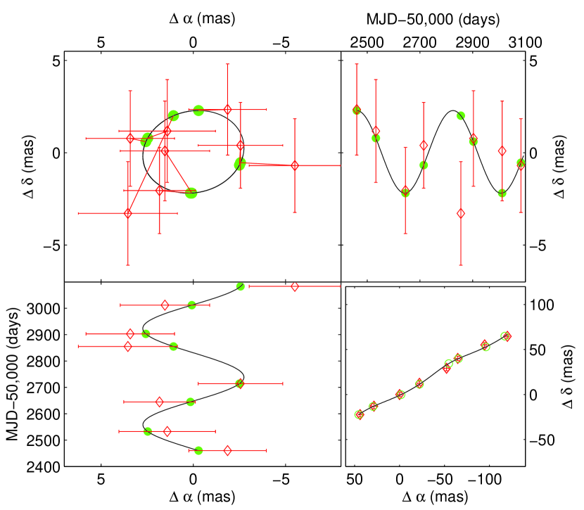
Figure 6.— Parallax of RX J0720.4$-$3125. Upper left: parallactic ellipse showing motion in Right Ascension versus that in Declination with the proper motion removed. The filled circles are the predicted positions of RX J0720.4$-$3125, and the open diamonds are the data. The data are connected to the predicted positions at the same epoch. Upper right: motion in Declination versus time with the proper motion removed. Lower left: motion in Right Ascension versus time with the proper motion removed. Lower right: motion in Right Ascension and Declination including the proper motion.

5. Discussion

The distance $d=360^{+170}_{-90}$ pc we measure is roughly consistent with the estimate of $250\pm 25~{}$pc made by Posselt et al. (2006) comparing the hydrogen column density to RX J0720.4$-$3125 — as inferred from fits to its X-ray spectrum — with the run of hydrogen column with distance — as inferred from sodium columns to stars with known distances. Conversely, our parallax measurement indicates that the column density inferred from the spectral fits, which necessarily depends on the form assumed for the intrinsic spectrum, is reasonable (if perhaps slightly low; a distance slightly closer than the parallax distance is also found for RX J1856.5$-$3754: Posselt et al. (2006) find $d=135\pm 25$ pc, while our preliminary parallax yields $167^{+18}_{-15}$ pc).

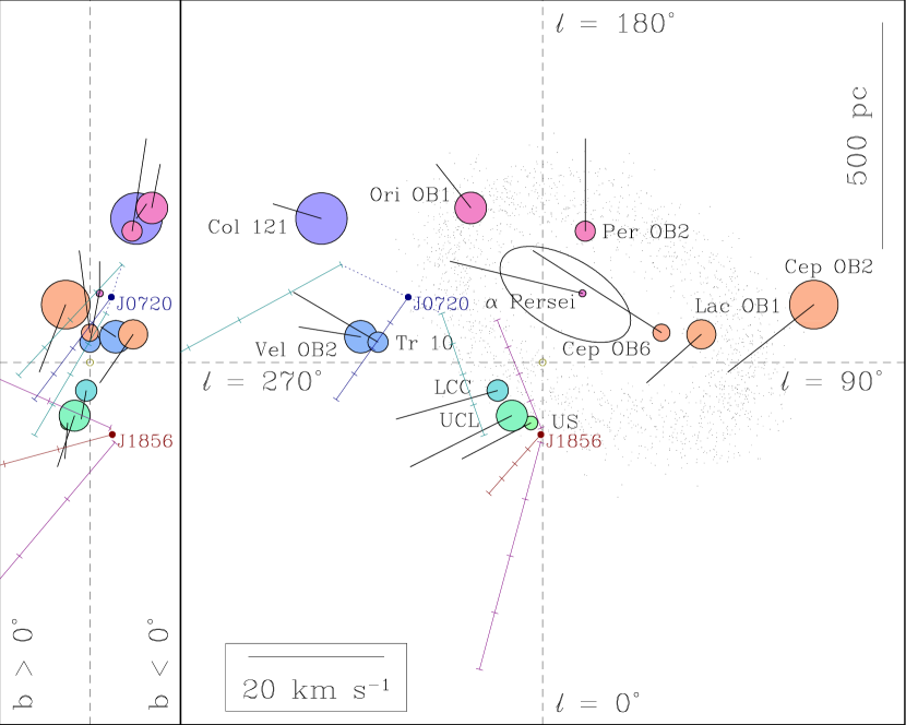
Figure 7.— Origins of two nearby isolated neutron stars. This figure, adapted from Fig. 29 of de Zeeuw et al. (1999), shows a view looking down on the Galactic plane (right panel, with Galactic longitude $\ell$ as indicated) and a view across the plane (left panel, with Galactic latitude $b$ as indicated). The filled circles show kinematically detected OB associations (filled circles; de Zeeuw et al. 1999) along with their streaming motions, and the scattered dots represent the Gould Belt (Olano, 1982). The present locations of RX J1856.5$-$3754 (Kaplan et al. 2002b; van Kerkwijk et al. 2006, in prep.) and RX J0720.4$-$3125 (this work) are indicated, as are trajectories back in time for the nominal distance and proper motion, assuming radial velocity $v_{\rm rad}=0$, as well as using the 1$\sigma$ distance limits and $v_{\rm rad}=\pm 0.935v_{\perp}$ (see § 5.1). The tick marks along the trajectories occur every 0.5 Myr; Galactic acceleration is negligible over these timescales. The scale for velocity of $20\mbox{ km s}^{-1}$ for the associations is shown along the bottom, while the linear scale of 500 pc is along the right edge. For reference, a source with a velocity of $20\mbox{ km s}^{-1}$ will traverse 500 pc in 25 Myr.

Our parallax implies that RX J0720.4$-$3125 is roughly a factor two more distant than RX J1856.5$-$3754. This agrees well with the simple estimate of KvKA02, which was based on the first-order assumptions that the optical flux for different sources scaled as $F_{\nu}\propto T(R/d)^{2}$, that the radii were similar, and that the temperature $T$ in the region emitting optical photons scaled with the temperature determined from fits to the X-ray spectra. Although this agreement may be a coincidence, it suggests that the mismatch between black-body fits to the X-ray and optical emission arises because the surface does not emit like a black body (i.e., that the temperatures in the layers of the atmosphere emitting X-ray and optical photons are different but related; e.g., Motch et al. 2003; Zane, Turolla, & Drake 2004), and not because the optical and X-ray emission originate in separate hot and cool regions (e.g., Braje & Romani 2002).

While the X-ray spectrum and flux of RX J0720.4$-$3125 had been observed to be relatively constant for years after its discovery (like for the other INS), observations in 2002 and 2003 showed a surprising spectral change (de Vries et al., 2004; Vink et al., 2004). The spectrum hardened significantly, although the flux stayed relatively constant. Our ACS observations occurred during the same time span. In § 2.4, we looked for variability in the optical flux of RX J0720.4$-$3125, but did not find any. This may not be entirely unexpected, however, if the optical flux indeed results from the Rayleigh-Jeans tail of some hot region (and scales as $R^{2}T$, as above). Over the course of our observations, the temperature of the X-ray blackbody changed by 6%, from $kT=88.3\pm 0.3$ keV (2002 November) to $93.8\pm 0.4$ keV (2004 May), while the blackbody angular diameter dropped $\sim\!6$% over the same period (Haberl et al., 2006). This implies a decrease in optical flux of $\sim\!6\%=0.07$ mag, which is smaller than our photometric uncertainty of 0.09 mag (Table 1). Even binning the observations we do not see significant variability: comparing the mean of epochs 1–4 with 5–8 there is a decrease of 0.08 mag, but the uncertainties on each mean are 0.05 mag.

5.1. Origin and Age

With the distance and proper motion of RX J0720.4$-$3125, we can estimate the space motion and try to determine its origin and age. As the simplest estimate, we determine the time required for RX J0720.4$-$3125 to reach its current location out of the Galactic plane. The current Galactic latitude is $b=-8.16\arcdeg$, and the proper motion in that coordinate is $\mu_{b}=-59.3\mbox{ mas yr}^{-1}$. So, assuming it started at $b=0$, it has taken $\sim\!b/\mu_{b}=5\times 10^{5}$ yr to reach that height. However, this value is rather inaccurate. At a distance of $360$ pc, RX J0720.4$-$3125 is at $z-z_{\odot}=-50.7$ pc, where $z$ is the height above the Galactic plane, and the Sun is at $z_{\odot}\approx 10$ pc compared to local OB stars (Reed, 1997; Elias et al., 2006). So RX J0720.4$-$3125 is actually at $z\approx-40$ pc below the mid-plane. Given that this is comparable to the local scale-height of 30–40 pc of OB stars (Reed, 2000; Elias et al., 2006), we cannot actually use this method for a useful age estimate, but can only derive a rough upper limit of $\sim\!1$ Myr.

We can derive a more meaningful estimate from considering not simply the scale height of the OB population, but instead the actual locations of individual associations. In Fig. 7, we show the nearby Galactic OB associations (taken from de Zeeuw et al. 1999), and overdraw the current location and the previous motion of RX J0720.4$-$3125 for the distance corresponding to the best-fit parallax and zero radial velocity $v_{\rm rad}$. We also show the result for distances corresponding to $\pi\pm\sigma_{\pi}$, and for $v_{\rm rad}=\pm 0.935v_{\perp}$, where $v_{\perp}=185{\rm~{}km\,s^{-1}}$ is the velocity in the plane of the sky inferred from the proper motion and best-fit parallax, and the numerical factor $\cot(\cos^{-1}0.683)=0.934$ corresponds to the expected $1\sigma$ range in $v_{\rm rad}$ for random orientations. In our estimates of the space velocity, we corrected for the Sun’s motion relative to the Local Standard of Rest, of $(U,V,W)_{\odot}=(10.00,5.25,7.17){\rm~{}km\,s^{-1}}$ (Dehnen & Binney, 1998), as well as for differential galactic rotation, using Oort constants $(A,B)=(14.82,-12.37){\rm~{}km\,s^{-1}\,kpc^{-1}}$ (Feast & Whitelock, 1997). For comparison, we also show the location and motion of RX J1856.5$-$3754 (using $[\mu_{\alpha},\mu_{\delta}]=[0.327,-0.059]{\rm~{}mas\,yr^{-1}}$ and $\pi=6.0\pm 0.6{\rm~{}mas}$ [van Kerkwijk, Kaplan, & Anderson 2007, in preparation]).

From Fig. 7, one sees that, as discussed in Walter (2001), RX J1856.5$-$3754 plausibly came from the Upper Scorpius or Upper Scorpius Lupus OB association $\sim\!0.4$ Myr ago. For RX J0720.4$-$3125, as suggested by Motch et al. (2003) and Kaplan (2004), an origin in the Trumpler 10 (Tr 10) OB association $\sim\!0.7$ Myr ago seems likely. This is plausible in $\ell$, $b$, and distance, with little radial velocity required (values between $-20$ and $+50\mbox{ km s}^{-1}$ are compatible with the nominal distance). An origin in the Vela OB2 association is less likely but not impossible; it would imply a slightly smaller age ($\sim\!0.6$ Myr). For a substantially larger radial velocity ($\gtrsim\!500\mbox{ km s}^{-1}$), origins in the Lower Centaurus Crux, Upper Centaurus Lupus, or Upper Scorpius OB association are possible. Even for those, however, the age would still be below 1 Myr (as it has to be from the the proper motion in galactic latitude, see above; Fig. 7 shows that an age in excess of 1 Myr is excluded also for RX J1856.5$-$3754).

Overall, among all of the OB associations, an origin in Tr 10 seems most likely, with RX J0720.4$-$3125 approaching within $\sim\!17$ pc of the core (the radius of the association is $\sim\!30$ pc). This should be compared to 70 pc for Vela OB2, although this is a larger association with a radius of $\sim\!55$ pc. Of course, the fact that the trajectory points back to Tr 10 could be a coincidence. To estimate the probability of such a coincidence, we did a simulation where we assumed proper motions with the observed magnitude but with random direction on the sky. For each direction, we computed the minimum possible separation achieved among all OB associations from de Zeeuw et al. (1999), as well as the required radial velocity. We find that we can get RX J0720.4$-$3125 to within 25 pc (comparable to the closest approach to Tr 10) of any OB association in only 5% of our trials, and in only 2% of our trials if we restrict the radial velocity to $|v_{\rm rad}|\leq 350\mbox{ km s}^{-1}$ (which is almost $2v_{\perp}$). If we allow for the fact that some OB associations are larger than others, we find that in only 10% of our trials does RX J0720.4$-$3125 approach within the nominal radius, and in only 5% of our trials for the restricted radial-velocity range. If we vary also the magnitude of the proper motion, we obtain similar results. Therefore, given the small size of Tr 10 and the closeness of the approach, we consider it likely that RX J0720.4$-$3125 came from Tr 10.

If we accept an origin in Tr 10, the main uncertainty in the age comes from our distance uncertainty. To assess this, we drew parallaxes for RX J0720.4$-$3125 from a normal distribution corresponding to our measurement uncertainty, and determined what radial velocity and age gave the closest approach to Tr 10. We found, as expected, a most probable age of 0.7–0.8 Myr, and a linear relation between parallax and age such that ${\rm Age}=0.7\left(\pi/2.8\mbox{ mas}\right)\mbox{ Myr}$. We thus infer an $1\sigma$ range in age of 0.5–1.0 Myr. Larger parallaxes imply more negative radial velocities (approaching $-100\mbox{ km s}^{-1}$), while small parallaxes require high positive radial velocities (up to $400\mbox{ km s}^{-1}$ for $\pi<2$ mas) to get RX J0720.4$-$3125 to the distance of Tr 10 in the short time allowed.

The age we infer for RX J0720.4$-$3125 is comparable to simple estimates based on models of neutron star cooling (e.g., Kaplan et al., 2002a), but it poses a pair of puzzles. The first is that the spin-down age for RX J0720.4$-$3125 of 1.9 Myr is a factor of 2–3 larger than either the cooling age or our kinematic age (see Kaplan & van Kerkwijk 2005a and van Kerkwijk & Kaplan 2006, who also discuss possible explanations). In this respect, RX J0720.4$-$3125 may not be unique: the hotter neutron star RX J1308.6+2127 (catalog RX J1308.6+2127) has a similarly long spin-down age of 1.5 Myr (Kaplan & van Kerkwijk, 2005b). The second possible puzzle is that, kinematically, RX J0720.4$-$3125 appears older than RX J1856.5$-$3754, while its temperature is higher. Thus, the sources likely differ in some other aspect. The inferred magnetic field strengths are indeed different ($\sim\!2$ vs. $\lesssim\!1\times 10^{13}$ G; KvKA02; Kaplan & van Kerkwijk 2005a), but this may not suffice. Instead, it may reflect a small difference in mass, to which cooling appears to be especially sensitive (for a review, see Yakovlev & Pethick 2004).

6. Conclusions

We have measured the geometric parallax to the neutron star RX J0720.4$-$3125 with HST to a precision of 30%, with an additional systematic uncertainty of $\sim\!15$%. To our knowledge, at $B=26.6~{}$mag, RX J0720.4$-$3125 is the faintest optical object for which a parallax has been measured. While the measurement is too uncertain to lead to useful constraints on the radius (which would also require better model atmospheres), it helps greatly to set the demographic scale of the INS as a population relative to that of the radio pulsars, for which parallaxes of this magnitude have been measured routinely (using Very Long Baseline Interferometry [e.g., Chatterjee et al. 2004] for regular pulsars and “timing” parallaxes [e.g., van Straten et al. 2001] for millisecond pulsars). Furthermore, the astrometry shows that the space velocities of RX J0720.4$-$3125 and RX J1856.5$-$3754 are typical for radio pulsars (Arzoumanian, Chernoff, & Cordes 2002; Faucher-Giguère & Kaspi 2006).

The prospect for small improvements of the parallax are good, as a few measurements with a large time baseline will significantly constrain the proper motions of RX J0720.4$-$3125 and the reference stars, which will improve the epoch registration, reduce the systematic uncertainties (App. B.6), and reduce the parallax uncertainty through its covariance with the proper motion and reference position (Table 6). With such measurement, total (statistical plus systematic) uncertainties around 20% may be possible. To do much better, however, would require further intense observations, and more than 100 orbits of HST.

Until a more accurate distance is available, the best constraints will probably arise if the data are combined with our improved distance for RX J1856.5$-$3754 (van Kerkwijk et al. 2006, in prep.). While RX J0720.4$-$3125 has the poorer distance, in other ways the modeling is more constrained, since we know the spin period (but see Tiengo & Mereghetti 2007), have an estimate of its dipole magnetic field strength, and can use the variation with viewing geometry and the broad absorption feature in the X-ray spectrum (Haberl et al., 2004a).

At present, the most useful aspect of our measurement may be that they provide the necessary input for placing RX J0720.4$-$3125 on a cooling diagram; previously, this was done with an erroneous spin-down age, which disagrees with our kinematic age and leads to the object appearing hotter than predicted (e.g., Page et al., 2004). Of course, for proper comparison, we must be careful to construct cooling curves that reflect what we know about the surface composition (partially-ionized hydrogen? see van Kerkwijk & Kaplan 2006) and magnetic field ($\sim\!2\times 10^{13}$ G; Kaplan & van Kerkwijk 2005a) of RX J0720.4$-$3125.

Appendix A Details of the Parallax Fitting

Our method of determining the parallax from the position measurements in individual exposures was described briefly in § 4. Here, we describe it in more detail.

We measured positions using the effective-PSF (ePSF) technique, as discussed in AK04 and § 2.2, and this gives us 64 measurements of up to 23 stars. In order to determine the parallax of RX J0720.4$-$3125, it is necessary to transform and combine those measurements. We did this in two stages: (i) combine measurements from different exposures in each epoch; and (ii) fit the resulting averages with an astrometric model.

The first stage starts with distortion-corrected positions $(x,y)_{Ees}$ and the associated uncertainties $(\sigma_{x},\sigma_{y})_{Ees}$, where $E=1\ldots N_{\rm epoch}$ is the epoch, $e=1\ldots N_{\rm exp}$ is the exposure, and $s=1\ldots N_{\rm star}$ is the star number, and the uncertainties are inferred from the ePSF fit (§ 2.2). For each epoch $E$, we determine average transformations to a common frame by solving for six parameters $\{(\Delta x,\Delta y)_{Ee},\psi_{Ee},\eta_{Ee},\psi_{y,Ee},\eta_{y,Ee}\}$, which relate averaged positions $(x,y)_{Es}$ in the common frame to the model positions $(\hat{x},\hat{y})_{Ees}$ in each exposure, by

$$\hat{x}_{Ees} = (1+\eta_{Ee})\left[(x_{Es}-\Delta x_{Ee})\cos\psi_{Ee}+(y_{Es}-\Delta y_{Ee})\sin\psi_{Ee}\right],$$

$$\hat{y}_{Ees}^{\prime} = (1+\eta_{Ee})\left[-(x_{Es}-\Delta x_{Ee})\sin\psi_{Ee}+(y_{Es}-\Delta y_{Ee})\cos\psi_{Ee}\right],$$

$$\hat{y}_{Ees} = (1+\eta_{y,Ee})\left[-\hat{x}_{Ees}\sin\psi_{y,Ee}+\hat{y}_{Ees}^{\prime}\cos\psi_{y,Ee}\right].$$ (A1)

Here, $(\Delta x,\Delta y)_{Ee}$ are the offsets of each exposure compared to the common frame, $\psi_{Ee}$ is the difference in rotation, $\eta_{Ee}$ is the difference in plate-scale, and $\psi_{y,Ee}$ and $\eta_{y,Ee}$ are additional parameters that represent the non-orthogonality of the $x$ and $y$ axes and the difference between the scales of those axes. Note that while we use all six parameters in general, we also made trials with the scale difference and non-orthogonality fixed to zero; see App. B.4.

In our fits, we take the common frame to be the first exposure, i.e., for this exposure all transformation parameters are zero, and one has $(\hat{x},\hat{y})_{E1s}=(x,y)_{Es}$. We solve for the remaining transformation parameters and the average positions $(x,y)_{Es}$ at the same time, using a numerical $\chi^{2}$ minimization routine (mrqmin from Press et al. 1992) to minimize,

$$\chi^{2}=\sum_{s=1}^{N_{\rm star}}\sum_{e=1}^{N_{\rm exp}}\left[\left(\frac{x_{Ees}-{\hat{x}}_{Ees}}{\sigma_{x,Ees}}\right)^{2}+\left(\frac{y_{Ees}-{\hat{y}}_{Ees}}{\sigma_{y,Ees}}\right)^{2}\right].$$ (A2)

To verify whether our fits our reasonable, we use the global $\chi^{2}$ value, and compute $\chi^{2}$ values for individual exposures and stars. For a more direct comparison with our input uncertainties $\sigma_{Ees}$, we also calculate the standard deviation for individual sources,

$$s^{2}_{x,Es}=\frac{1}{N_{\rm exp}-1}\sum_{e=1}^{N_{\rm exp}}\left({\hat{x}}_{Ees}-x_{Es}\right)^{2}.$$ (A3)

and the same for $y$. Since $N_{\rm exp}$ is sometimes small for a given star, the standard deviation is not always a good estimator of the true uncertainty, but on average we have found that it is quite reasonable (see § B.2 and Fig. 8).

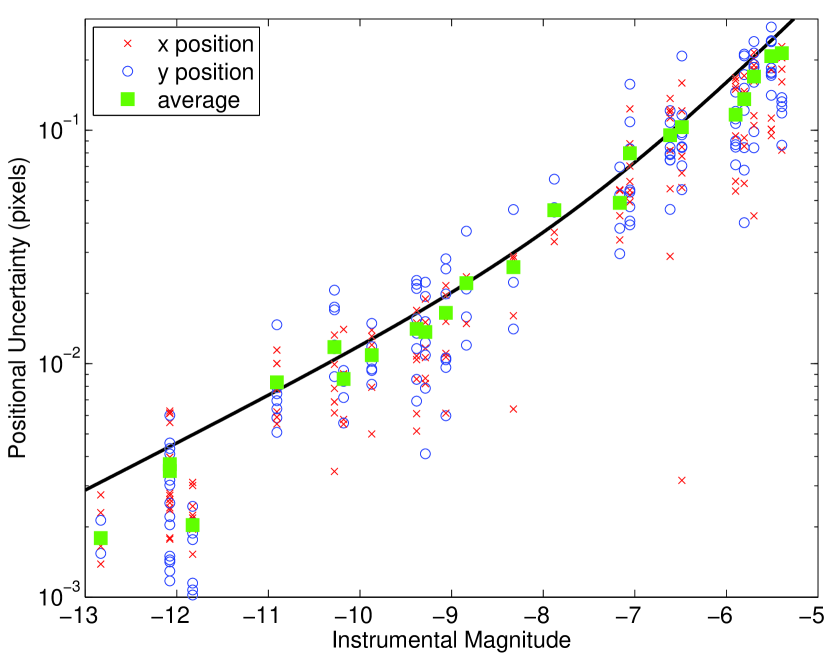
Figure 8.— Positional uncertainty in pixels versus instrumental magnitude for the HRC data—compare to Fig. 1 from KvKA02 and Fig. 2 from AK04. We show the standard deviations of the individual positions around the average position for each epoch (Eq. A3), in both $x$ (crosses) and $y$ (open circles). We also show the root-mean-square average of all the $x$ and $y$ standard deviations (filled squares). Note that for the brightest stars, the standard deviations are expected to underestimate the true measurement uncertainties (App. A). The curve gives the relation expected from our simulations (Eq. B1). The simulations may also underestimate the true uncertainty at the brightest magnitudes (App. B.2).

In considering $\chi^{2}$ values and standard deviations for individual exposures and objects, one has to keep in mind that the transformation parameters and the average positions are not independent. In our case, the four brightest stars (A, B, 118, and 119) dominate the fit. These provide eight measurements per exposure (4 in each coordinate), but there are six free transformation parameters, and hence the fit will partly adjust to remove measurement errors. As a result, the $\chi^{2}$ for these sources are often much less than $2N_{\rm exp}-2$, the value one would expect if the transformation were independent of the average positions. For fainter stars, however, which have much less effect on the transformation, ones does expect (and we find) $\chi^{2}\simeq 2N_{\rm exp}-2$. Of course, for the same reason, the standard deviations calculated using Eq. A3 will underestimate the true measurement uncertainties for the brightest stars.

Since we fit for all parameters at the same time, the above covariances are taken into account automatically. For instance, for star 119, our fit yields errors $\sigma_{Es}$ on the average position similar to the input uncertainty $\sigma_{Ees}$ for a single measurement; this is a consequence of the fact that substantial variation in the average position can be compensated for by changes in the transformation parameters. In contrast, for fainter stars, we find $\sigma_{Es}\simeq\sigma_{Ees}/\sqrt{N_{\rm exp}}$, as one would expect for averaging $N_{\rm exp}$ exposures using a fixed transformation. Nevertheless, we worried about our transformation being dominated by just a few stars, especially since their formal measurement uncertainties are very small, as low as 0.003 pix for star 119, at which level systematic effects may well dominate. Thus, in App. B.2, we verify that our results are robust to variations in the weight assigned to the brightest stars.

After the combination of the exposures, we have a set of $(x,y)_{Es}$ along with their uncertainties. We also have a set of times $t_{E}$ (which determine parallactic offsets $[\Delta\alpha_{\pi},\Delta\delta_{\pi}]_{E}$ computed using either the JPL DE200 ephemeris or the approximate formulae of Cox 2000, p. 670; both methods gave identical final results) and initial guesses for the position angle ${\rm PA}_{E}$ (based on the data headers; Table 1) and plate-scale scale_E ($28.27\mbox{ mas pixel}^{-1}$; AK04). In our second stage of the parallax determination, we want to solve for the full set of stellar parameters $\mathcal{S}_{s}$ and epoch transformations parameters $\mathcal{E}_{E}$.

The stellar parameters $\mathcal{S}_{s}$ are the reference celestial position $(\Delta\alpha,\Delta\delta)_{s}$ of star $s$ relative to star A at time $t_{0}$ (note that we chose equal scales for $\Delta\alpha$ and $\Delta\delta$, so no $\cos\delta$ term is needed), the proper motion $(\mu_{\alpha},\mu_{\delta})_{s}$, and the parallax $\pi_{s}$ (for individual stars, the proper motion or parallax may be fixed or set to zero). In terms of these parameters, the celestial position of star $s$ at epoch $E$ is given by,

$$\Delta\hat{\alpha}_{Es} = \Delta\alpha_{s}+\mu_{\alpha,s}(t_{E}-t_{0})+\pi_{s}\Delta\alpha_{\pi,E},$$

$$\Delta\hat{\delta}_{Es} = \Delta\delta_{s}+\mu_{\delta,s}(t_{E}-t_{0})+\pi_{s}\Delta\delta_{\pi,E},$$ (A4)

For the exposures, the parameters $\mathcal{E}_{E}$ are the position $(x_{0},y_{0})_{E}$ on the detector of the reference position (i.e., $[\Delta\alpha,\Delta\delta]=[0,0]$, or the [model] position of star A), the difference $\phi_{E}$ between the initial guess ${\rm PA}_{E}$ for the position angle and the fitted value, the difference $\lambda_{E}$ between the initial guess ${\rm scale}_{E}$ for the plate-scale and the fitted value, and additional parameters $\phi_{y,E}$ and $\lambda_{y,E}$ that represent the non-orthogonality of the $x$ and $y$ axes and the difference between the scales of those axes. With these parameters, the transformation from the celestial position of each star at each epoch $(\Delta\hat{\alpha},\Delta\hat{\delta})_{Es}$ to the model positions $(\hat{x},\hat{y})_{Es}$ is given by,

$$\hat{x}^{\prime}_{Es} = {\rm scale}_{E}^{-1}(1+\lambda_{E})\left[-\Delta\hat{\alpha}_{Es}\cos\left({\rm PA}_{E}+\phi_{E}\right)+\Delta\hat{\delta}_{Es}\sin\left({\rm PA}_{E}+\phi_{E}\right)\right],$$

$$\hat{y}^{\prime}_{Es} = {\rm scale}_{E}^{-1}(1+\lambda_{E})\left[\Delta\hat{\alpha}_{Es}\sin\left({\rm PA}_{E}+\phi_{E}\right)+\Delta\hat{\delta}_{Es}\cos\left({\rm PA}_{E}+\phi_{E}\right)\right],$$

$$\hat{x}_{Es} = x_{0,E}+\hat{x}^{\prime}_{Es},$$

$$\hat{y}_{Es} = y_{0,E}+(1+\lambda_{y,E})\left[-\hat{x}^{\prime}_{Es}\sin\phi_{y,E}+\hat{y}^{\prime}_{Es}\cos\phi_{y,E}\right].$$ (A5)

Note that our transformation uses 6 parameters (as does that of AK04), not just the normal four parameters of reference position, position angle, and scale, but we can also set $\phi_{y,E}=\lambda_{y,E}=0$ to have a four-parameter transformation (see App. B.4).

In the fit, we use Eqs A4 and A5 to calculate predicted positions, and fit simultaneously for $\mathcal{E}_{E}$ and $\mathcal{S}_{s}$ by minimizing,

$$\chi^{2}=\sum_{s=1}^{N_{\rm star}}\sum_{E=1}^{N_{\rm epoch}}\left[\left(\frac{x_{Es}-{\hat{x}}_{Es}}{\sigma_{x,Es}}\right)^{2}+\left(\frac{y_{Es}-{\hat{y}}_{Es}}{\sigma_{y,Es}}\right)^{2}\right].$$ (A6)

This expression is very similar to the one for the combination of the exposures (Eq. A2), the only difference being that for the combination the positional parameters (the average positions) were independent of exposure number, while here there is a dependence on the time of each epoch (Eq. A4). Because of this similarity, our implementation uses the same fitting routine for both steps.

Note that the above method departs from that used by KvKA02, which solved first for $\mathcal{E}_{E}$, then $\mathcal{S}_{s}$, and iterated. We found that while our iterative solution was not biased, direct minimization was more precise, could more correctly disentangle the effects of stellar proper motions and uncertainties in $\mathcal{E}_{E}$, and found more easily the global $\chi^{2}$ minimum.

Our fit automatically yields a global $\chi^{2}$, but, like for the exposure combination, we can also calculate $\chi^{2}$ values for each individual star (Table 4) and each individual epoch (Table 5), and these are useful in identifying problems. We stress again, however, that these are not rigorous $\chi^{2}$ values, because the exposure parameters $\mathcal{E}_{E}$ are common to all of the stars, and the $\chi^{2}$ for a single star does not take this into account (similarly, $\mathcal{S}_{s}$ are common to all of the epochs, and the $\chi^{2}$ for a single epoch does not take this into account). As for the combinations, this affects the brightest stars in particular; from Table 4, one indeed sees that stars A, B, 118, and 119 have $\chi^{2}_{\rm red}$ substantially below unity.

Appendix B Alternate Schemes for the Parallax Measurement

We made a number of choices in determining the positions of stars in individual exposures and in combining these positions measurements. While we had reasons to prefer some schemes over others, we wished to verify that our final measurements did not depend on the detailed choices that we made. Therefore, we present the consequences of different ways of measuring positions (§ B.1), estimating uncertainties (§ B.2), identifying “bad” measurements (§ B.3), and combining exposures into averages and fitting these to an astrometric model (§ B.4). We also discuss a few statistical tests of the robustness of our results (§ B.5) and end with a summary of the possible sources of systematic error (§ B.6).

We note that all of the steps in the analysis (§ 2.2, § 4, and App. A) were performed independently by two of us (DLK and MHvK), using separate routines. We cross-checked the results at many points in the analysis, ensuring results were identical.

B.1. Alternate Position Measurements

At the start of the project, we wished to see if the measurement scheme of AK04 (Appendix C) was optimal. We did a number of experiments, and settled on a slightly different scheme, described in § 2.2. Overall, we found that, for our project, the choice of scheme had little influence: differences in the final parallax were less than 0.15 mas, and we find the same parallax also if we simply use the routines provided by AK04 and do careful rejection of outliers (App. B.3). However, the differences may be important for brighter sources, and hence we briefly describe our experiments below.

First, we varied the way pixels are weighted, taking into account only Poisson noise, as in AK04, also read-noise, or even a small, few percent “flat-field” error (proportional to the flux). We found that using just read-out and Poisson noise provided superior $\chi^{2}$ for the combination of exposures. We also tried determining weights based on the ePSF model instead of the observed counts. Here, using observed counts has the disadvantage that statistical fluctuation towards low (high) counts get too high (low) a weight), while using a model has the problem that, due to focus changes, etc., the model may not be precise. The results, however, where not significantly different.

Second, we experimented with the fit region, trying the $5\times 5$ pixel box used by AK04, smaller and larger boxes, as well as circular regions with a range of radii. Overall, we found that circular regions gave slightly smaller residuals in combining exposures. We picked a radius of 2.56 pixels to minimize the dependence of the number of pixels in the region on centroid position (the average number included is 20.6, with a standard deviation of 0.7).

Third, we tried determining the sky from annuli around sources, like AK04 do, including it in the fitting process, and fixing it globally to the header value mdrizsky. We found only slight differences; our choice of a constant sky level was based on a slightly smaller $\chi^{2}$.

Fourth, we tried fitting for the ePSF amplitude as well as fixing these amplitudes using the average photometry and an aperture correction for each exposure. It had minimal effect: using fixed amplitudes gave $\chi^{2}$ worse by a few percent in the combination and astrometry.

B.2. Alternate Uncertainty Schemes

We determined uncertainties in the positions from the $\chi^{2}$ fitting. To verify these, we simulated the detection of 10,000 stars of a range of brightnesses, and calculated standard deviations. This simulation included the effects of photon noise and read noise (which dominate for the fainter stars), but did not include any mismatches in the ePSF (which will dominate for brighter stars). We find that the 1$\sigma$ uncertainty in each coordinate can be described approximately by,

$$\sigma(m_{\rm i})=\left[\left(C_{1}10^{m_{\rm i}/5.0}\right)^{2}+\left(C_{2}10^{m_{\rm i}/2.5}\right)^{2}\right]^{1/2}~{}{\rm pixel},$$ (B1)

where $m_{\rm i}=-2.5\log N$ with $N$ the counts in a $5\times 5$ pixel box (or, equivalently, the ePSF amplitude from the fit), and $C_{1}\simeq 1.14$ and $C_{2}\simeq 36$ are constants determined from the simulation. This relation roughly matches expectations, since the uncertainty should scale as the full-width at half-maximum (FWHM) divided by the signal-to-noise ratio (SNR), where the SNR has contributions from Poisson noise ($\propto\sqrt{N}$; first term, which dominates for bright stars) and read-noise ($\propto N/{\rm RN}$; second term, which dominates for faint stars; here, ${\rm RN}$ is the read-noise in the pixels covered by the PSF). With a gain of unity for flat-fielded images and a FWHM close to 1 pixel, one expects $C_{1}\simeq 1$, as we find. Similarly, from the read-noise of $\sim\!6{\rm~{}DN}$ per pixel, and considering that 20 pixels are used, one roughly reproduces $C_{2}$. In Fig. 8, we compare the predictions with the standard deviations found after combination of the exposures (Eq. A3), and find good agreement.

For the brightest stars, one might expect that systematic effects to start to dominate, but from neither simulations nor observations do we find evidence for this (Fig. 8), in contrast to what KvKA02 found for WFPC2 data, and what is found for HRC by AK04. For the observations, however, one has to keep in mind that, for the brightest stars, the standard deviations underestimate the measurement uncertainty, since part of the measurement error has been absorbed in the transformations required to put the exposures on a single reference frame (App. A). Hence, any systematic error might be hidden in the transformations.

To test the effect of possible systematic errors, we added, in quadrature, constant terms of up to 0.01 pixel to our input uncertainties, thus reducing the weight carried by the brightest stars. As expected, the overall $\chi^{2}$ for the exposure combination and the astrometry decreases, from $\chi^{2}_{\rm red,comb}=\sum_{E}\chi^{2}_{E}/\sum_{E}N_{{\rm dof},E}=1.21$ and $\chi^{2}_{\rm red,par}=1.07$ to 0.89 and 0.81, respectively. The change in parallax, however, is only 0.005 mas. We can use these results to estimate the size of the systematic errors, by determining for what additional systematic error one obtains $\chi^{2}_{\rm red}\simeq 1$. We find this is at about 0.007 pix, consistent with the results of AK04.

B.3. Alternate Rejection Schemes

During our analysis, we found that a very important part in obtaining a good registration is the rejection of measurements that are biased by a bad pixel or a cosmic ray. The scheme we used was meant to be as objective as possible, being based on identifying bad pixels in an entirely automatic way. Yet, we still needed to reject some additional measurements (§ 2.2). As an alternative, we identified bad measurements from large deviations of the positions and/or instrumental magnitudes of single observations from the average. We did not employ a formal rejection criterion but examined all of the data manually, iteratively registering the exposures and removing outliers. For the brightest four stars, very few exposures were rejected, while for the fainter ones we included on average 7 exposures per epoch. With this set, we derived a parallax very similar to our best value.

B.4. Alternate Combination Schemes

We combine our individual measurements into averages using a six-parameter transformation between exposures, and again use a six-parameter transformation in our astrometric solution. Although these choices are grounded in the work of AK04, we tried some alternatives: (i) combining exposures with two or four-parameter transformations; (ii) tying the epochs using a four-parameter transformation; and (iii) instead of merging the exposures, treating each exposure as a separate epoch, and fit for 64 transformations $\mathcal{E_{E}}$ simultaneously.

We found that a different choice of combining the exposures did not change the final parallax significantly (i.e., by more than 0.1 mas), although it did affect the quality of the fit: with fewer parameters, the $\chi^{2}$ values were significantly higher. Using only 4 parameters for the astrometric tie has a more drastic effect on the quality of the fit. The parallax, however, decreased by only 0.1 mas compared to our main result.

When we treated all exposures as separate epochs, we found a parallax identical to within 0.01 mas with that derived using our two-stage approach. The fit was formally less good than our two-stage result, which may reflect an underestimate of the uncertainties of bright stars and/or remaining position measurements contaminated by cosmic rays. We made a number of experiments to address these issues, but, fortunately, the effects of all of them on the parallax is small, $<0.1$ mas.

B.5. Statistical Tests

As a statistical measure of the robustness of our result, we tried to “jackknife” our data, removing either one star or one epoch from the fit. Removing a single star does not change the fit appreciably, showing that no single star dominates the fit. On average, there was no change in the parallax, and the dispersion was only 0.03 mas. The dispersion is dominated by one star, B: with B omitted, the parallax decreased by 0.1 mas (note that B is also the most discrepant point in Fig. 4). Given how small this change is compared to the statistical uncertainty, we are satisfied with this test.

Removing an epoch had a more dramatic effect. As can be seen from Fig. 6, some epochs fit significantly better than others. Specifically, removing epoch 5 improved the quality of the fit ($\chi^{2}_{\rm red,par}=0.93$ for the overall transformation), and increased the parallax to $3.32\pm 0.96$ mas. In contrast, removing epoch 8 gave a less significant change in the quality of the fit ($\chi^{2}_{\rm red,par}=1.03$), but a larger change in parallax, to $1.67\pm 1.01$ mas. These were the most extreme examples: the mean shift was 0.08 mas, and the standard deviation was 0.5 mas (0.3 mas excluding the epoch 8 result). Part of the problem with removing epoch 8 seems to be a covariance with the proper motion: while removing the other epochs changed the proper motion by $<\!1\sigma$, removing epoch 8 changed $\mu_{\alpha}$ to $-91.9\pm 1.5\mbox{ mas yr}^{-1}$ (the correlation coefficients between $\pi$ and $\mu_{\alpha}$ or $\mu_{\delta}$ are significant; see Table 6).

Finally, we also removed individual exposures when we fit using all of the exposures without combination (App. B.4). Again, the mean of the parallaxes was identical to that in Table 6, and the standard deviation was 0.1 mas. This leads to an uncertainty of 0.9 mas for the parallax (following Efron & Tibshirani 1993), which is the same as what we derived from error propagation.

B.6. Estimate of the Systematic Uncertainties

The biggest source of systematic uncertainties that could affect our results are the epochs that we include. While the other choices, as described above, led to parallax differences of $<\!0.1$ mas, the jackknife tests on epochs gave larger changes (App. B.5). Overall, we believe our result from Table 6 to be reliable, but we should add a systematic uncertainty to the statistical uncertainty quoted there. The magnitude of this uncertainty should be similar to the variation in the parallax that we see, or 0.4 mas. This may be an overestimate, as our exposure jackknife tests indicated that the bias was small, but we prefer to err on the conservative side. A small number of measurements in the future that will have a long enough time baseline to make the proper motion better determined should reduce this uncertainty significantly.

References

- Anderson & King (2004) Anderson, J. & King, I. 2004, Multi-filter PSFs and Distortion Corrections for the HRC, HST Instrument Status Report 04-15, Space Telescope Science Institute, AK04
- Anderson & King (2000) Anderson, J. & King, I. R. 2000, PASP, 112, 1360
- Anderson & King (2006) —. 2006, PSFs, Photometry, and Astrometry for the ACS/WFC, HST Instrument Status Report 06-01, Space Telescope Science Institute
- Arzoumanian et al. (2002) Arzoumanian, Z., Chernoff, D. F., & Cordes, J. M. 2002, ApJ, 568, 289
- Braje & Romani (2002) Braje, T. M. & Romani, R. W. 2002, ApJ, 580, 1043
- Chatterjee et al. (2004) Chatterjee, S., Cordes, J. M., Vlemmings, W. H. T., Arzoumanian, Z., Goss, W. M., & Lazio, T. J. W. 2004, ApJ, 604, 339
- Cox (2000) Cox, A. N. 2000, Allen’s Astrophysical Quantities, 4th edn. (New York: AIP Press/Springer)
- de Vries et al. (2004) de Vries, C. P., Vink, J., Méndez, M., & Verbunt, F. 2004, A&A, 415, L31
- de Zeeuw et al. (1999) de Zeeuw, P. T., Hoogerwerf, R., de Bruijne, J. H. J., Brown, A. G. A., & Blaauw, A. 1999, AJ, 117, 354
- Dehnen & Binney (1998) Dehnen, W. & Binney, J. J. 1998, MNRAS, 298, 387
- Drake et al. (2002) Drake, J. J. et al. 2002, ApJ, 572, 996
- Efron & Tibshirani (1993) Efron, B. & Tibshirani, R. J. 1993, An Introduction to the Bootstrap (London: Chapman and Hall)
- Elias et al. (2006) Elias, F., Cabrera-Caño, J., & Alfaro, E. J. 2006, AJ, 131, 2700
- Faucher-Giguère & Kaspi (2006) Faucher-Giguère, C.-A. & Kaspi, V. M. 2006, ApJ, 643, 332
- Feast & Whitelock (1997) Feast, M. & Whitelock, P. 1997, MNRAS, 291, 683
- Fruchter & Hook (2002) Fruchter, A. S. & Hook, R. N. 2002, PASP, 114, 144
- Goudfrooij et al. (2006) Goudfrooij, P., Bohlin, R. C., Maiz-Apellaniz, J., & Kimble, R. A. 2006, PASP, 118, 1455
- Goudfrooij & Kimble (2002) Goudfrooij, P. & Kimble, R. A. 2002, in The 2002 HST Calibration Workshop, ed. S. Arribas, A. Koekemoer, & B. Whitmore (Baltimore: Space Telescope Science Institute), 105
- Haberl (2004) Haberl, F. 2004, in XMM-Newton EPIC Consortium meeting, Palermo, 2003 October 14-16 (astro-ph/0401075)
- Haberl (2006) Haberl, F. 2006, in Isolated Neutron Stars: from the Interior to the Surface, ed. D. Page, R. Turolla, & S. Zane (Springer) (astro-ph/0609066)
- Haberl et al. (1997) Haberl, F., Motch, C., Buckley, D. A. H., Zickgraf, F.-J., & Pietsch, W. 1997, A&A, 326, 662
- Haberl et al. (2003) Haberl, F., Schwope, A. D., Hambaryan, V., Hasinger, G., & Motch, C. 2003, A&A, 403, L19
- Haberl et al. (2006) Haberl, F., Turolla, R., de Vries, C. P., Zane, S., Vink, J., Méndez, M., & Verbunt, F. 2006, A&A, 451, L17
- Haberl et al. (2004a) Haberl, F., Zavlin, V. E., Trümper, J., & Burwitz, V. 2004a, A&A, 419, 1077
- Haberl et al. (2004b) Haberl, F. et al. 2004b, A&A, 424, 635
- Jehin et al. (2006) Jehin, E., O’Brien, K., & Szeifert, T. 2006, FORS 1+2 User Manual, VLT-MAN-ESO-13100-1543 78, European Southern Observatory
- Kaplan (2004) Kaplan, D. L. 2004, Ph.D. Thesis, California Institute of Technology
- Kaplan et al. (2002a) Kaplan, D. L., Kulkarni, S. R., van Kerkwijk, M. H., & Marshall, H. L. 2002a, ApJ, 570, L79
- Kaplan & van Kerkwijk (2005a) Kaplan, D. L. & van Kerkwijk, M. H. 2005a, ApJ, 628, L45
- Kaplan & van Kerkwijk (2005b) —. 2005b, ApJ, 635, L65
- Kaplan et al. (2002b) Kaplan, D. L., van Kerkwijk, M. H., & Anderson, J. 2002b, ApJ, 571, 447, KvKA02
- Kaplan et al. (2003) Kaplan, D. L., van Kerkwijk, M. H., Marshall, H. L., Jacoby, B. A., Kulkarni, S. R., & Frail, D. A. 2003, ApJ, 590, 1008
- Koekemoer et al. (2002) Koekemoer, A. M., Fruchter, A. S., Hook, R. N., & Hack, W. 2002, in The 2002 HST Calibration Workshop, ed. S. Arribas, A. Koekemoer, & B. Whitmore (Baltimore: Space Telescope Science Institute), 337
- Kulkarni & van Kerkwijk (1998) Kulkarni, S. R. & van Kerkwijk, M. H. 1998, ApJ, 507, L49
- Lattimer & Prakash (2000) Lattimer, J. M. & Prakash, M. 2000, Phys. Rep., 333, 121
- Momany et al. (2006) Momany, Y., Zaggia, S., Gilmore, G., Piotto, G., Carraro, G., Bedin, L. R., & de Angeli, F. 2006, A&A, 451, 515
- Motch & Haberl (1998) Motch, C. & Haberl, F. 1998, A&A, 333, L59
- Motch et al. (2005) Motch, C., Sekiguchi, K., Haberl, F., Zavlin, V. E., Schwope, A., & Pakull, M. W. 2005, A&A, 429, 257
- Motch et al. (2003) Motch, C., Zavlin, V. E., & Haberl, F. 2003, A&A, 408, 323
- Olano (1982) Olano, C. A. 1982, A&A, 112, 195
- Page et al. (2004) Page, D., Lattimer, J. M., Prakash, M., & Steiner, A. W. 2004, ApJS, 155, 623
- Pavlovsky et al. (2006) Pavlovsky, C. et al. 2006, ACS Data Handbook (Baltimore: Space Telescope Science Institute), Version 5.0
- Posselt et al. (2006) Posselt, B., Popov, S., Haberl, F., Trümper, J., Turolla, R., & Neuhäuser, R. 2006, in Isolated Neutron Stars: from the Interior to the Surface, ed. D. Page, R. Turolla, & S. Zane (Springer) (astro-ph/0609275)
- Press et al. (1992) Press, W. H., Teukolsky, S. A., Vetterling, W. T., & Flannery, B. P. 1992, Numerical recipes in C. The art of scientific computing, 2nd edn. (Cambridge: University Press)
- Proffitt et al. (2002) Proffitt, C. R., Davies, J. E., Brown, T. M., & Mobasher, B. 2002, in The 2002 HST Calibration Workshop, ed. S. Arribas, A. Koekemoer, & B. Whitmore (Baltimore: Space Telescope Science Institute), 201
- Reed (1997) Reed, B. C. 1997, PASP, 109, 1145
- Reed (2000) —. 2000, AJ, 120, 314
- Schlegel et al. (1998) Schlegel, D. J., Finkbeiner, D. P., & Davis, M. 1998, ApJ, 500, 525
- Sirianni et al. (2005) Sirianni, M. et al. 2005, PASP, 117, 1049
- Stetson (1987) Stetson, P. B. 1987, PASP, 99, 191
- Tiengo & Mereghetti (2007) Tiengo, A. & Mereghetti, S. 2007, ApJ, 657, L101
- van Kerkwijk & Kaplan (2006) van Kerkwijk, M. H. & Kaplan, D. L. 2006, in Isolated Neutron Stars: from the Interior to the Surface, ed. D. Page, R. Turolla, & S. Zane (Springer) (astro-ph/0607320)
- van Kerkwijk et al. (2004) van Kerkwijk, M. H., Kaplan, D. L., Durant, M., Kulkarni, S. R., & Paerels, F. 2004, ApJ, 608, 432
- van Kerkwijk & Kulkarni (2001) van Kerkwijk, M. H. & Kulkarni, S. R. 2001, A&A, 380, 221
- van Straten et al. (2001) van Straten, W., Bailes, M., Britton, M., Kulkarni, S. R., Anderson, S. B., Manchester, R. N., & Sarkissian, J. 2001, Nature, 412, 158
- Vink et al. (2004) Vink, J., de Vries, C. P., Méndez, M., & Verbunt, F. 2004, ApJ, 609, L75
- Voges et al. (1999) Voges, W. et al. 1999, A&A, 349, 389
- Walter (2001) Walter, F. M. 2001, ApJ, 549, 433
- Walter & Lattimer (2002) Walter, F. M. & Lattimer, J. M. 2002, ApJ, 576, L145
- Yakovlev & Pethick (2004) Yakovlev, D. G. & Pethick, C. J. 2004, ARA&A, 42, 169
- Zacharias et al. (2004) Zacharias, N., Urban, S. E., Zacharias, M. I., Wycoff, G. L., Hall, D. M., Monet, D. G., & Rafferty, T. J. 2004, AJ, 127, 3043
- Zane et al. (2005) Zane, S., Cropper, M., Turolla, R., Zampieri, L., Chieregato, M., Drake, J. J., & Treves, A. 2005, ApJ, 627, 397
- Zane et al. (2002) Zane, S., Haberl, F., Cropper, M., Zavlin, V. E., Lumb, D., Sembay, S., & Motch, C. 2002, MNRAS, 334, 345
- Zane et al. (2004) Zane, S., Turolla, R., & Drake, J. J. 2004, Advances in Space Research, 33, 531 (astro-ph/0308326)