The stellar initial mass function of metal-rich populations 111To appear in The Metal Rich Universe, La Palma, Canary Islands, June 12th–16th, 2006, G. Israelian & G. Meynet (eds.), Cambridge University Press
Abstract
Does the IMF vary? Is it significantly different in metal-rich environments than in metal-poor ones? Theoretical work predicts this to be the case. But in order to provide robust empirical evidence for this, the researcher must understand all possible biases affecting the derivation of the stellar mass function. Apart from the very difficult observational challenges, this turns out to be highly non-trivial relying on an exact understanding of how stars evolve, and how stellar populations in galaxies are assembled dynamically and how individual star clusters and associations evolve. -body modelling is therefore an unavoidable tool in this game: the case can be made that without complete dynamical modelling of star clusters and associations any statements about the variation of the IMF with physical conditions are most probably wrong. The calculations that do exist demonstrate time and again that the IMF is invariant: There exists no statistically meaningful evidence for a variation of the IMF from metal-poor to metal-rich populations. This means that currently existing star-formation theory fails to describe the stellar outcome. Indirect evidence, based on chemical evolution calculations, however indicate that extreme star-bursts that assembled bulges and elliptical galaxies may have had a top-heavy IMF.
1 Introduction
The stellar initial mass function (IMF), , where is the stellar mass, is the parent distribution function of the masses of stars formed in one event. Here, the number of stars in the mass interval is . Salpeter (1955) inferred the IMF from solar-neighbourhood star-counts applying corrections for stellar evolution and Galactic-disk structure finding , for . Miller & Scalo (1979) and Scalo (1986) derived the IMF for using better data and a more sophisticated analysis establishing that the IMF flattens or turns-over at small masses. Modern studies of solar-neighbourhood star-count data which also apply detailed corrections for unknown multiple systems in the star-counts, confirm that for (Kroupa, Tout & Gilmore 1993; Kroupa 1995b; Reid, Gizis & Hawley 2002). Using spectroscopic star-by-star observations, Massey (2003) reports the same slope or index for in many OB associations and star clusters in the Milky Way (MW), the Large- and Small-Magellanic clouds (LMC, SMC, respectively). It is therefore suggested to refer to as the Salpeter/Massey slope or index. It is valid for .
The IMF is, strictly speaking, a hypothetical construct because any observed system of stars merely constitutes a particular representation of a distribution function. The probable existence of a unique can be inferred from observations of many ensembles of such systems (e.g. Massey 2003). If, after corrections for
(a) stellar evolution,
(b) unknown multiple stellar systems and
(c) stellar-dynamical biases,
the individual distributions of stellar masses is similar within the statistical uncertainties, then we (the community) deduce that the hypothesis that the stellar mass distributions are not the same can be excluded. That is, we make the case for a universal, standard or canonical stellar IMF within the physical conditions probed by the relevant physical parameters (metallicity, density, mass) of the populations at hand.
This canonical IMF is a two-part-power law, the only structure with confidence found so far being the change of index from the Salpeter/Massey value to a smaller one near :
| (1) |
It has been fully corrected for unknown multiple stellar systems in the low-mass () regime, while multiplicity corrections in the high-mass regime await to be done. The evidence for a universal upper mass cutoff near (Weidner & Kroupa 2004; Figer 2005; Oey & Clarke 2005; Koen 2006) seems to be rather well established in populations with metallicities ranging from the LMC () to the super-solar Galactic centre () such that the stellar mass function (MF) simply stops at that mass. This mass needs to be understood theoretically (see discussion in Kroupa & Weidner 2005).
Chabrier (2003) offers a log-normal form222Note that the log-normal form is physically better motivated in the sense that a physical process will not abruptly change a slope as in the canonical IMF, but it also needs to be extended by a power-law above to meet the needs of the observational data thereby losing its advantage. A reason why the author prefers to use the canonical form is mathematical simplicity and the ease with which parts of it can be changed without affecting other parts. which fits the canonical form quite well (e.g. Romano et al. 2005).
Below the hydrogen-burning limit, there is substantial evidence that the IMF flattens further to (Kroupa 2001a; Kroupa 2002; Chabrier 2003). Therefore, the canonical IMF most likely has a peak at . Brown dwarfs, however, comprise only a few % of the mass of a population and are therefore dynamically irrelevant. Note that the logarithmic form of the canonical IMF, , which gives the number of stars in log-intervals, also has a peak near . However, the system IMF (of stellar companions per binary combined to system masses) has a maximum in the mass range (Kroupa et al. 2003).
The above form has been derived from detailed considerations of local star-counts thereby representing an average IMF: for low-mass stars it is a mixture of stellar populations spanning a large range of ages ( Gyr) and metallicities ([Fe/H]), while for the massive stars it constitutes a mixture of different metallicities ([Fe/H]) and star-forming conditions (OB associations to very dense star-burst clusters: R136 in the LMC). Therefore it can be taken to be a canonical form, and the aim is to test whether even more extreme star-forming conditions such as found in super-metal rich environments or super-dense regions may deviate from it. Any systematic deviations of the IMF with physical conditions of the environment would constrain our understanding of star formation, would give us a prescription of how to set-up stellar-dynamical systems, and last not least would allow more precise galaxy-formation and evolution calculations.
2 The expectation: the IMF must depend on star-formation environment and in particular on the metallicity
There are two basic arguments suggesting that the IMF ought to be dependent on the physical conditions of star formation:
2.1 The Jeans-mass argument
A) A region of a molecular cloud undergoing gravitational collapse will have over-dense sub-regions within it which are also Jeans-unstable collapsing independently to form smaller structures which themselves may again sub-fragment (e.g. Zinnecker 1984). Ultimately stars result. The essence of this concept is that a region spanning a Jeans length which has at least a Jeans mass undergoes gravitational collapse. The Jeans mass depends on the temperature and density of the cloud, (e.g. Larson 1998; Bonnell, Larson & Zinnecker 2006). Now, in metal-rich environments there is more dust and therefore the collapsing gas can cool more effectively reducing and increasing . Thus,
| (2) |
B) The fact that the IMF is not a featureless power-law but has structure in the mass range suggests there to be a characteristic mass of a few .
Bonnell et al. (2006) suggest that this characteristic mass of fragmentation may be a result of the coupling of gas to dust such that there is a change from a cooling equation of state, where while the density increases, to one with slight heating at high densities, . Again, this implies a dependency of the characteristic mass on the metallicity through the cooling rate:
| (3) |
There seems to be observational evidence supporting the notion that stellar masses are derived from Jeans-unstable mass fragments: pre-stellar cloud cores are found to be distributed like the canonical IMF in low-mass star formating regions (Motte, Andre & Neri 1998; Testi & Sargent 1998; Motte et al. 2001; but see Nutter & Ward-Thompson 2006).
While the concept of the Jeans mass is very natural and allows one to nicely visualise the physical process of fragmentation, it has the problem that the densest regions of a pre-star-cluster cloud core ought to have the smaller fragment masses, but instead the most massive stars are seen to form in the densest regions.
2.2 The self-limitation argument
A rather convincing physical model of the IMF which avoids the problem with the Jeans mass argument has been suggested by Adams & Fatuzzo (1996) and Adams & Laughlin (1996). The argument here is that the Jeans mass has virtually nothing to do with the final mass of a star because structure in a molecular cloud exists on all scales. Therefore, no characteristic density can be identified, and “no single Jeans mass exists”. When a cloud region becomes unstable a hydrostatic core forms after the initial free-collapse. This core then accretes at a rate dictated by the physical conditions in the cloud. The metallicity influences the accretion rate through the sound velocity (higher sound velocity, larger accretion rate) by steering the cooling rate (more metals more dust lower smaller sound velocity). The many physical variables describing the formation of a single star have distributions, and folding these together yields finally an IMF in broad agreement with a log-normal shape (as also shown by Zinnecker 1984). This fails though at large masses, where the IMF is a power-law and where additional physical processes probably play a role (coagulation, competitive accretion). The important point however is that this theory also expects a variation of the resulting characteristic mass with metallicity as above:
| (4) |
2.3 Robust implication?
Thus, both theoretical lines of argument seem to suggest the same qualitative behaviour, namely that the IMF ought to shift to smaller characteristic masses with increasing metallicity. This would therefore seem to suggest a very robust if not fundamental expectation of star-formation theory.
Is it born out by empirical evidence? The best way to test this theoretical expectation is to measure the IMF in metal-poor environments and to compare to the shape seen in metal-rich environments.
A measurement of the IMF in a population with super-solar abundance would be especially important. Unfortunately this is extremely difficult, because populations with super-solar abundances are exceedingly rare. Only one star-cluster with [Fe/H] is known, NGC 6791, but its ancient age of Gyr implies it to be dynamically very old. Evaporation of low-mass stars will thus have significantly affected the shape of the present-day mass function, which has not been measured yet (King et al. 2005). Other metal-rich environments constitute the central MW region (§ 5.2) and galactic spheroids (§ 5.3), the latter allowing only indirect evidence on the IMF through their chemical properties.
In general, measurements of the IMF are hard, because stellar masses can only be inferred indirectly through their luminosity, , which also depends on age, metallicity and the star’s spin angular momentum vector, collectively producing a distribution of for a given . The empirical knowledge that can be gained about the IMF is discussed next.
3 The shape of the IMF
3.1 The local stellar sample
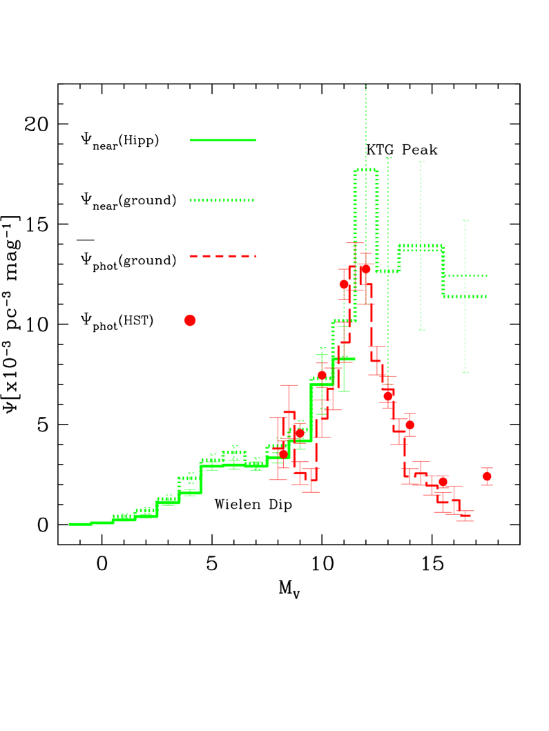
The best knowledge about the IMF we glean from the local volume-limited stellar sample. The basic technique is to construct the stellar luminosity function (LF), , where is the stellar absolute magnitude in some photometric pass band (we are stuck with magnitudes rather than working with the physically more intuitive luminosities due to our historical inheritance). The number of stars within the complete volume in the magnitude interval is then . These are the same stars as enter from above, and thus results our master equation
| (5) |
The observable is which we get from the sky. Our target is , and the hurdle is the derivative of the stellar mass–luminosity relation, . This is quite problematical, because we can only get at by either constructing observational mass–luminosity relations using extremely well-observed binary stars with known Kepler solutions which nevertheless have uncertainties that are magnified when considering the derivative, or we can resort to theoretical stellar models which give us well defined derivatives but depend on theoretically difficult processes within stellar interiors (opacities, convection, rotation, magnetic fields, equation of state, nuclear energy generation processes).
There are two basic local LF’s: (I) We can count all stars within a trigonometrically-defined distance limit such that the stellar sample is complete, i.e. we can see all stars of magnitude within a distance . The volume-limited sample for solar-type stars having excellent parallax measurements extends to pc, while for the faintest M-dwarfs pc (Reid, Gizis & Hawley 2002). Tests of completeness are made by comparing the stars with within to the number of these stars in a volume element further out (Henry et al. 2002), finding that faint stars remain to be discovered even within a distance of 5 pc. For this nearby LF, , the stars are well scrutinised on an individual-object basis, and geometric distances are known to within about 10 per cent. At the faint end is badly constrained resting on only a few stars.
(II) Prompted by the “discovery” of large amounts of dark matter in the MW disk (Bahcall 1984)333The evidence for dark matter within the solar vicinity disappeared on closer scrutiny (Kuijken & Gilmore 1991)., novel deep surveys were pioneered by Reid & Gilmore (1982). This second-type of sampling can be obtained by performing deep, pencil-beam photographic or CCD imaging surveys through the Galactic disk. From the images the typically 100 or so main sequence stars need to be gleaned using automatic image-, colour and brightness recognition systems. The distances of the stars are determined using the method of photometric parallax, which relies on estimating the absolute luminosity of a star from its colour, and then calculating its distance from the distance modulus. The resulting flux-limited sample of stars has photometric-distance limits within which the counts are complete. The distance limits decrease for fainter stars.
Clearly, while only one nearby LF exists, many photometric LFs can be constructed for different fields of view. Each observation yields a few dozen to hundreds of stars, and so the overall sample size becomes very significant. The various surveys have shown to be invariant with direction. This should, of course, be the case, since the Galactic-field stars with an average age of about 5 Gyr have a velocity dispersion of about 25-50 pc/Myr such that within 200 Myr a volume with a dimension of the survey volumes (a few hundred pc) is completely mixed.
It therefore came as a surprise that and are significantly different at faint luminosities (Fig. 1).
3.2 The mass–luminosity relation
When not understanding something the best strategy to continue is sometimes to simply “forget” the problem and continue the path of least resistance. Thus, while the problem could not be explained immediately, it turned out to be constructive to first ascertain which LF shape must be the correct one using entirely different arguments.
In eq. 5 the slope of the stellar mass–luminosity relation of stars enters posing a clue. Fig. 2 in Kroupa (2002) shows the mass–luminosity data of binary stars with Kepler orbits, and demonstrates that a non-linearity exists near such that a pronounced peak in appears at with an amplitude and width essentially identical to the maximum seen in the photometric LF at this luminosity (Fig. 1). This agreement of
-
1.
the location of the maximum and
-
2.
the amplitude and
-
3.
the width of the extremum
convincingly suggest stellar astrophysics to be the origin of the peak in the LF, rather than the MF. The Wielen dip (Fig. 1) similarly results from subtle structure in the mass–luminosity relation. Thus, simply by counting stars on the sky we are able to direct our gaze within their interiors: It is the internal constitution of stars which changes with changing main-sequence mass and this is what drives the structure in the mass–luminosity relation.
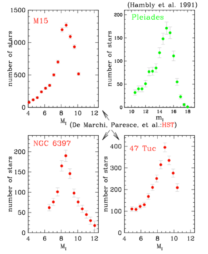
Having thus established that the peak in the LF must, in fact be there where it is also found as a result of fundamental astrophysical processes, we can test this result using star-clusters which constitute single-age, single-metallicity and equal-distance stellar samples. Fig. 2 does exactly this, and indeed, a very pronounced peak is evident at exactly the right location and with the right width and height (Kroupa 2002: fig. 1).
We can therefore trust the peak in . In Fig. 1 it can be seen that also shows evidence for this peak, noting that the peak is smeared apart in the local stellar sample because the stars have a wide spread in metallicities. The metallicity-dependence of the peak has been shown to be in agreement with the LFs of star clusters over a large range of metallicity (von Hippel et al. 1996; Kroupa & Tout 1997).
Kroupa, Tout & Gilmore (1993) then performed a trick to get at the correct mass–luminosity relation without having to resort to theoretical or purely empirical relations which are very uncertain in their derivatives (Kroupa 2002: fig. 2): The Malmquist-corrected is used to define the amplitude and width and location of the extremum in the single-age, single-metallicity average , and integrating the resulting constraint leads to a semi-empirical relation. It is a semi-empirical relation because we used theoretical stellar models to place, one can say, zeroth order constraints on this relation, i.e. to prove the existence of the extremum and to estimate its location and width and amplitude. With this theoretical knowledge in-hand we then used the LF to constrain the detailed run of . The result is in amasing agreement even with the most recent high-quality binary-star constraints by Delfosse et al. (2000). With the so-obtained relation, which has the correct derivative, it is now possible to take another step towards constraining the MF.
But first the problem needs to be addressed.
3.3 Unresolved binary systems
One bias clearly affecting are unresolved multiple systems; in constructing all stellar companions have been counted individually, while consists of “stars” too far away to be resolved if they are multiple. Also, a faint companion star may not be seen because it lies below the flux limit while the primary enters the formal photometric distance limit. Furthermore, an unresolved binary system appears redder unless both stars are of equal mass and this affects the calculated stellar space density because the photometric distance is misjudged. All the effects can and must be corrected for; this having been done thoroughly for the first time by Kroupa et al. (1993).
The bias due to unresolved binaries affecting can be nicely demonstrated using realistic numbers for the multiplicity in the Galactic field (Goodwin et al. 2006): Suppose the observer sees 100 systems on the sky. Of these 40 are binaries, 15 triples and 5 quadruples. The multiplicity fraction is . The observer will construct the LF using these 100 systems, but in fact 85 stars are missed. All of these are much fainter than their primary, implying a non-linear depression at the faint end of the LF.
3.4 The standard Galactic-field IMF
Together with a thorough modelling of the star-formation history of the solar neighbourhood (low-mass stars take long to descend to the main sequence), local Galactic disk structure and metallicity spreads, as well as different fractions of multiple stars and photometric and trigonometric distance uncertainties, Kroupa et al. (1993) performed a multi-dimensional optimisation for the parameters of a two-part-power law MF. The result is one MF which unifies both and . It is given by eq. 1 for (Kroupa et al. 1993; Reid et al. 2002). Adopting this IMF as being correct, Kroupa (1995b) also showed that the observed LFs are arrived at if stars are born as binaries in clusters which evolve and disperse their stellar content into the Galactic field. Chabrier (2003) further points out that non-linearities in the colour–magnitude relation used in photometric parallax adds to the underestimate of the stellar densities at the faint end of .
Scalo (1986) had performed a very detailed analysis of the stellar mass function, which was superseded for through new star-count data and the new modelling described above. But for his analysis remains valid. Using star counts out to kpc distances for early-type stars he modelled their spatial distribution and took account of their production through different star-formation rates, and arrived at an estimate of the Galactic-field IMF adopted in Kroupa et al. (1993):
| (6) |
Together with eq. 1 this is the standard Galactic-field IMF. Elmegreen & Scalo (2006) then showed that there can be artificial features in the massive-part of the Galactic-field IMF when it is deduced from the present-day field MF under varying star-formation rates (SFRs), frustrating attempts to attribute any possible structure there to star-formation physics.
3.5 The canonical IMF
As already stated in § 1, the IMF for early-type stars can also be inferred for individual OB associations and star clusters. Massey (2003 and previous papers) has shown the IMF for massive stars to be independent of density ( stars/pc3, the densest cluster being R136 in the LMC) and metallicity (, the population with the lowest metal abundance being in the SMC). It always has , thus leading to the standard or canonical stellar IMF, eq. 1.
The question now emerges as to why for . This is referred to as the “Scaslo vs Massey discrepancy”.
Considering the uncertainties, it would be valid to discard the difference. However, using the standard Galactic-field IMF in galactic evolution models would yield about 3 times fewer stars in the mass range and about 8 times fewer stars with than when using the canonical IMF. So it is important to know . We will return to this later-on, but as before, when not immediately seeing a possible solution it often proves useful to ignore the problem until new insights open new avenues for exploration.
3.6 Massive stars come seldomly alone
Spectroscopic and speckle-interferometric observations of nearby massive star-forming regions have shown that OB stars prefer more than one partner (Zinnecker 2003; Goodwin et al. 2006). In particular, Preibisch et al. (1999) present the most detailed multiplicity study of the Orion Nebula Cluster (ONC) demonstrating that the rule are triples rather than binaries as amongst T Tauri stars.
This allows us to set-up the following hypothesis:
| (7) |
That is, Massey was observing dynamically less-evolved and therefore more binary-rich populations whereas Scalo saw the field population which is, to a significant extend, “contaminated” by runaway OB stars which are mostly single (Stone 1991). This would be a neat solution to our problem: fainter OB stars are hidden among their brighter primaries flattening the Massey-IMF, while the mostly single OB-field stars in the Scalo sample would be a more correct representation of the true IMF.
Thus we may be led to conclude that in actuality the true (binary-corrected) IMF is eq. 6 (), while eq. 1 () is wrong. This would, of course, have important implications for Galactic astrophysics as well as cosmology; most galaxy-formation and evolution calculations are being done with a Salpeter IMF.
4 Lessons from star clusters
Star clusters pose star-formation events which are extremely well correlated in space, time and chemistry, and so studying the MF within clusters avoids most of the problems we need to deal with in the Galactic field. However, there are a number of serious issues that essentially annihilate any advantage one might have gained by having an equal-age, -distance and -metallicity population:
4.1 Young clusters
To avoid dynamical evolution complicating the star-counts in a cluster, young clusters are chosen. However, uncertainties in pre-main sequence tracks make the calculation of stellar masses from stellar luminosities and colours or spectra very uncertain for ages less than a few Myr. Errors of about 50 % would not be untypical. These errors are not randomly distributed though, but cause systematic offsets from the true stars. And so unphysical structures appear in the MF. This is discussed in more depth in Kroupa (2002). Very young clusters also have a high binary fraction, which again would require corresponding corrections. Young clusters evolve very rapidly during the first 1 Myr as a result of residual gas expulsion. For example, the ONC with an age of about 1 Myr is already between 5 and 15 initial crossing times old, implying a rapid dynamical evolution of the binary population (fig. 1 in Kroupa 2000; fig. 9 in Kroupa et al. 2001) and an expansion of the cluster such that a substantial fraction of its initial population has probably been lost (Kroupa, Aarseth & Hurley 2001). This translates into a selective stellar-mass loss if the cluster was initially significantly mass-segregated (Moraux, Kroupa & Bouvier 2004). It is therefore never clear exactly which corrections have to be applied, and an inferred stellar MF is very likely not to be a good representation of the IMF.
4.2 Old clusters
To avoid the issues above (uncertain pre-main sequence theory, rapidly evolving stellar and binary populations), older clusters within which stars are on or close to the main sequence would appear to be useful. They are definitely useful, but such clusters are heavily evolved dynamically, and so the MF will not represent the IMF even for clusters with an age near 100 Myr. Unresolved multiple systems remain a problem, and for example for the Pleiades Stauffer (1984) shows that the fraction of photometric binaries is 26 % (these are stars that are more luminous than a single star of the same colour), while Kaehler (1999) notes that a true binary fraction between 60 and 70 % may be possible. Even globular clusters appear to have a sizeable binary population (e.g. Rubenstein & Bailyn 1997).
A star cluster which has managed to survive its initial gas expulsion phase re-virialises on a time-scale of tens of Myr (Kroupa et al. 2001). It’s binary population is depleted by then such that binaries with orbital Kepler velocities smaller than the velocity dispersion in the pre-expansion cluster will have been disrupted. The remaining binaries are mostly inert; sometimes energetic binary–single-star or binary–binary encounters near the cluster core eject 1–3 stars (e.g. a single star and the binary) from the cluster. The cluster’s evolution is, however, well described by classical dynamical evolution tracks, i.e. the surviving binaries are dynamically not important, as shown explicitly by Kroupa (1995c). During this long-lived phase the cluster evolves towards energy equipartition, which implies that the low-mass stars gain energy and thus move outwards becoming lost to the Galactic tide, while the more massive stars loose energy and segregate towards the center of the potential. This process never stops, i.e. a cluster never actually reaches energy equipartition and dynamical equilibrium. The consequence is that as the cluster ages, it’s MF becomes increasingly depleted in low-mass stars. This is nicely evident in low-mass clusters in terms of a flattening of the LF, while unresolved binaries remain a significant bias despite their dynamical unimportance (fig. 10 in Kroupa 1995c). Baumgardt & Makino (2003) study the evolution of the MF in much detail for massive star clusters without binaries. In their fig. 7 they nicely show how the MF changes its slope in dependence of the cluster’s dynamical age expressed in terms of the fraction of the time until cluster disruption: clusters that have passed 50 % of their disruption time have essentially a flat () MF for , while for older clusters becomes negative.
4.3 Massive stars in clusters
Two processes compete for all stellar masses, but are particularly pronounced for massive stars because of the involved energetics.
Mass segregation: If massive stars form throughout a forming star cluster energy equipartition will force them to segregate to the center within a timescale , where are the masses of the average star and the massive stars, and is the median two-body relaxation time, as detailed in Kroupa (2004). For example, for the ONC, Myr and such that Myr age of the ONC. No wonder that the ONC sports a beautiful Trapezium, although it may also have formed at the centre (Bonnell & Davies 1998).
Core decay: The massive stars at the cluster centre, which may have been born there or segregated there, form a short-lived small- core. It decays on a time-scale , where is the number of massive stars in the core and is its crossing time. Again, for the ONC, we find (Kroupa 2004) yr its age. So why does the Trapezium still exist?
4.4 A highly abnormal “IMF” in the Orion Nebula Cluster
Detailed -body computations confirm this time-scale problem (Pflamm-Altenburg & Kroupa 2006): The ONC also has a highly abnormal “IMF” - only 10 stars more massive than are found in it, while 40 would be needed to allow the very final remnant of the central core to be still visible today and to account for the mass of the most massive star, given the cluster-mass–maximal-mass relation observed to exist among young clusters (Weidner & Kroupa 2006).
This appears to be the rule rather than the exception, Pflamm-Altenburg & Kroupa (2006) discuss the older Upper Scorpius OB association which also shows a deficit of massive stars compared to the canonical IMF. Naively this may be taken as good evidence for a bottom-heavy present-day IMF in a relatively metal-rich environment, which would even be consistent qualitatively with the theoretical arguments of § 2 (higher-metallicity environments making lower-mass stars on average).
Further work, however, shows this to be an illusion: Pflamm-Altenburg & Kroupa (2006) apply a specially designed chain-regularisation code (CATENA) to study the dynamical stability of ONC-type cores, finding that if the ONC and Upper Scorpius OB association, which is understood to be an evolved version of the ONC, were born with 40 OB stars, then the observations are well-accounted for. Indeed, Stone (1991), among others, shows that 46 % of all O stars are probably runaways of which about 18 % have line-of-sight velocities pc/Myr. Energetic dynamical encounters in cluster cores therefore have a very significant effect on the shape of the “IMF” in clusters and OB associations. And, massive stars are rapidly dispersed from their birth sites with corresponding implications for the spreading of heavy elements and feedback-energy deposition throughout a galaxy.
The implications of these studies is therefore that the massive-star content of star clusters and OB associations is not a measure of the true initial content, unless the full dynamical history of the cluster or OB association is taken into account.
4.5 Summary
It would thus appear that clusters and OB associations of any age are a horrible place to study the IMF.
This does not mean, however, that these systems are useless. Quite on the contrary: they are indeed our only samples of stars formed together and are therefore the only samplings from the IMF that exist before dispersion into the field. The point of the above pessimistic note is to instill the fact that any measurement of the “IMF” in a cluster or association must be accompanied by a dynamical investigation before conclusions about the possible variation of the IMF can be made. An excellent example follows in § 5.2.
5 Evidence for variation of the IMF
The derivation of MFs in many clusters and associations leads to many values of measured over different stellar mass ranges. The alpha-plot, , can therefore give us information about the true shape of the putative underlying IMF, and also of the scatter about a mean IMF (Scalo 1998). This scatter can then be studied theoretically using the methods mentioned above, i.e. -body calculations of star-clusters with different properties. Thus, § 4.5 needs to be invoked in the context of some recent interesting observational studies that suggest the IMF to vary at low masses (e.g. Oasa et al. 2006) and at high masses (Gouliermis et al. 2005).
One important aspect here is the purely statistical scatter resulting from finite- sampling from a putative universal IMF (§ 1). Elmegreen (1997, 1999) showed that the observed scatter is consistent with the variations of as a result of sampling from the IMF. Stellar-dynamical and unresolved binary-star biases lead to systematic deviations of away from the true value, and Kroupa (2001, 2002) has shown the observed alpha-values to be consistent with the canonical IMF (eq. 1) for a large variety of stellar populations using theoretical models of initially binary-rich star clusters.
As already deduced with some force by Massey (2003, and previous papers), there is no evidence for systematic shifts of with metallicity nor density. At the one extreme end of the scale of physical conditions, globular clusters have very similar MFs as young Galactic clusters and the Galactic field, while constraints on the massive-star content of globular clusters are such that the IMF could not have been too top heavy as otherwise the mass-loss from evolving stars would have unbound the clusters (Kroupa 2001). At the other extreme end, the super-solar Arches cluster near the Galactic centre has a massive-star IMF again very similar to the Salpeter/Massey one (§ 5.2 below).
Kroupa (2002) studied the distribution, , of measured values for stars more massive than a few finding it to be describable by two Gaussians, one somewhat broad but with symmetric wings, and the other exceedingly narrow, and both centered on the Salpeter/Massey value . This is very surprising because the various values were obtained by different research groups observing different objects. An equivalent theoretical data set shows a somewhat broader unsymmetric distribution offset from the input Salpeter/Massey value. This needs further investigation, because one would expect the theoretical data to be better “behaved” than the observational ones which include the entire complications of inferring masses from observed luminosities. Concerning this open question, Maíz Apellániz & Úbeda (2005) point out that binning the star-counts into mass-bins of equal mass leads to biases that distort the shape of the IMF when the number of stars is small, which is often the case at high masses.
Returning to the empirically-determined existence of an upper mass limit to stars near (§ 1), it remains to be understood why it does not seem to depend on metallicity: Theoretical concepts would suggest that feedback ought to play a role in limiting the masses of stars, but this implicitly contains a metallicity dependence as the coupling of radiation to the accreting gas is more efficient in metal-rich environments. Thus, we are left yet again with two open questions.
5.1 Back to the “Scalo vs Massey discrepancy”
One important implication from this analysis of values for massive stars is that the above hypothesis (eq. 7) must be discarded: if unresolved multiple systems were the origin of the Scalo vs Massey discrepancy, then would have an asymmetric distribution stretching from the single-star value () to the unresolved binary-star value (). This is not the case. The Scalo vs. Massey discrepancy therefore is either non-existing (perhaps because Scalo’s analysis requires an update), or it has another hitherto unknown origin. The proposition by Elmegreen & Scalo (2006) that the IMF calculated from the present-day field MF may be steeper than the canonical IMF if the field was created during a lull in the star-formation rate deserves some attention in this context.
5.2 An example: The Galactic central region
Reports do exist that in extreme environments there is evidence for a top-heavy IMF. These often come from indirect arguments based on luminosity and available mass for star formation in star-bursts, for example: scaling the canonical IMF to the observed luminosity would lead to a mass in stars far superior to dynamical mass constraints from kinematics, requiring either a top-heavy (smaller ) IMF, or an IMF truncated typically near or above . Paumard et al. (2006) report evidence for a top-heavy IMF in both circum-nuclear disks in the MW. While the observations are quite convincing, § 4.5 needs to be invoked before taking such results as affirmative evidence for a variable stellar IMF.
A case in point is the Arches cluster at the Galactic centre, where the conditions for star formation are very different to those prevalent in the solar vicinity or the disk of the LMC, by being in general warmer ( K instead of 10 K) and having a super-solar metallicity ([Fe/H]).
Klessen, Spaans, Jappsen (2006) perform an excellent state-of-the art calculations of star-formation under such conditions. They state in their abstract: “In the solar neighbourhood, the mass distribution of stars follows a seemingly universal pattern. In the centre of the Milky Way, however, there are indications for strong deviations and the same may be true for the nuclei of distant star-burst galaxies. Here we present the first numerical hydro-dynamical calculations of stars formed in a molecular region with chemical and thermodynamic properties similar to those of warm and dusty circum-nuclear star-burst regions. The resulting initial mass function is top-heavy with a peak at , a sharp turn-down below and a power-law decline at high masses. We find a natural explanation for our results in terms of the temperature dependence of the Jeans mass, with collapse occurring at a temperature of K and an H2 density of a few cm-3, …”. Theirs would be in agreement with the previously reported apparent decline of the stellar MF in the Arches cluster below about .
Shortly after the above theoretical study appeared, Kim et al. (2006) published their observations of the Arches cluster and performed the necessary state-of-the art -body calculations of the dynamical evolution of this young cluster, revising our knowledge significantly. Quoting from their abstract: “We find that the previously reported turnover at is simply due to a local bump in the mass function (MF), and that the MF continues to increase down to our 50 % completeness limit () with a power-law exponent of for the mass range of . Our numerical calculations for the evolution of the Arches cluster show that the values for our annulus increase by 0.1-0.2 during the lifetime of the cluster, and thus suggest that the Arches cluster initially had a Gamma of – , which is only slightly shallower than the Salpeter value.” ().
This serves to illustrate the general observation that when detailed high-resolution observations and accurate -body calculations are combined, claims of abnormal IMFs tend to vanish, irrespective of what theory prefers to have. Another example, the ONC, has already been noted above.
5.3 Spheroids: old, very extreme star-bursts?
An interesting, albeit indirect, result by Francesca Matteucci and her collaborators based on multi-zone photo-chemical evolution studies of the MW, its Bulge and elliptical galaxies shows the MW disk to be re-producible by the standard Galactic-field IMF (eq. 6, ) but not the canonical IMF (eq. 1). This is supported by the independent work of Portinari, Sommer-Larsen & Tantalo (2004). In contrast, the MW Bulge may require a rapid phase of formation lasting 0.01–0.1 Gyr and a top-heavy IMF with (Romano et al. 2005; Ballero, Matteucci & Origlia 2006). For elliptical galaxies a similar scenario seems to hold, whereby the IMF needed to account for the colours and chemical properties is the canonical one (), but flattening (decreasing ) slightly with increasing galaxy mass (Pipino & Matteucci 2004). An experiment, where the yields for massive stars are changed as much as possible without violating available constraints confirms this result - it seems not to be possible to understand the metallicity distribution of MW Bulge stars with a standard Galactic field IMF. Instead, seems to be required (Ballero, Kroupa & Matteucci 2007). Nevertheless, uncertainties remain. Thus, Samland, Hensler & Theis (1997) find the Bulge to have formed over a time-span of about 4 Gyr with a Salpeter IMF using a two-dimensional chemo-dynamical code, while Immeli, Samland & Gerhard (2004) obtain formation time-scales near 1 Gyr using a three-dimensional chemo-dynamical code. Finally, Zoccali et al. (2006) find the “MW bulge to be similar to early-type galaxies, in being -element enhanced, dominated by old stellar populations, and having formed on a timescale shorter than 1 Gyr”. “Therefore, like early-type galaxies the MW bulge is likely to have formed through a short series of starbursts triggered bythe coalescence of gas-rich mergers, when the universe was only a few Gyr old”. For low-mass stars, Zoccali et al. (2000) find the Bulge to have a similar MF as the disk and globular clusters.
5.4 Composite populations
The “Scalo vs Massey discrepancy” found in § 3.5 and its proposed solution in § 3.6 in terms of unresolved multiple systems was found, in § 5.1, not to be possible. Again, as in § 3.5 we might argue that trying to solve the discrepancy is not worth the effort, given the uncertainties. Indeed, the probable solution drops-out through an entirely different line-of-thought:
It needs to be remembered that star clusters are the fundamental building blocks of galaxies (Kroupa 2005). Therefore, to be exact, all the stellar IMFs in all the clusters forming in one “star-formation epoch” (Weidner, Kroupa & Larsen 2004) of a galaxy must be added to calculate the global, galaxy-wide “integrated galactic IMF” (IGIMF). This has been pointed-out by Vanbeveren (1982, 1984) and discussed again by Scalo (1986), and formulated for an entire galaxy by Kroupa & Weidner (2003, 2005), noting that the star-clusters are distributed as a power-law embedded-cluster mass function with an exponent , where the Salpeter value would be 2.35. Also, an empirical relation exists limiting the mass of the most massive star in a cluster with stellar mass : (Weidner & Kroupa 2006), enhancing the IGIMFIMF effect.
Putting this together, an integral over all clusters formed together in one epoch results, and the composite IMF turns out to be steeper with (the canonical IMF value) for with a steep downturn at a mass . Both, and the galaxy-wide maximum star mass, , depend on the star-formation rate of the galaxy, and so the situation becomes complex with important implications for galactic spectro-photometric and chemical evolution studies given that the number of supernovae of type II is depressed significantly per unit stellar mass formed when compared to a universal Salpeter IMF, which is often assumed in cosmological applications (Goodwin & Pagel 2004; Weidner & Kroupa 2005). Koeppen, Weidner & Kroupa (2006) show that this IGIMF-ansatz naturally explains the observed form of the mass–metallicity relation of galaxies without the need to invoke selective outflows (which are not excluded though).
Applied to the MW, Scalo’s comes-out naturally for an input canonical IMF. This is also required by spectro-photometric and chemical-evolution models of the MW disk (§ 5.3). At the same time, for LSB galaxies the IGIMF must be steep, i.e. bottom-heavy. Again, this seems to be confirmed by observations (Lee et al. 2004). Is this, then, the solution to the “Scalo vs Massey discrepancy”?
Elmegreen (2006), however, opposes the notion that the IGIMF is different to the stellar IMFs found in individual clusters, mostly because the star-cluster mass function is not steep steep enough (), in which case as already shown by Kroupa & Weidner (2003). Much therefore rests on the detailed shape of the star-cluster initial mass function ! Also, the existence of a physical relation is of central importance to the argument, but opposing views are being voiced (e.g. Elmegreen 2006). An argument against IGIMF IMF is that some studies suggest these to be equal, e.g. in elliptical galaxies (§ 5.4). However, an appreciable fraction of the research which Elmegreen fields in-support of his equality-conjecture actually support the inequality-conjecture. So this issue is still very much under debate and may need observational improvement by (i) better constraining the true initial star-cluster mass function and (ii) improving the empirical relation. Observational work is underway to test the IGIMFIMF notion, and for example Selman & Melnick (2005) find the composite IMF to be flatter than the stellar IMF in the 30 Dor star-forming region, as predicted, but only with low-significance.
6 Concluding remarks
It would have seemed that when two mutually more or less exclusive theories of the origin of stellar masses make the same basic prediction concerning the variation of the average stellar mass with physical conditions, that this expected variation would be very robust and born out in observational data. Alas, the observational data on the IMF are resilient - they do not yield what we desire to see. The stellar IMF is invariant and can be best described by a two-part power-law form (eq. 1). This holds true for metallicities ranging from those of globular clusters to super-solar values near the Galactic centre, and for densities less than about stars/pc3. Even the maximal stellar mass of about seems to be independent of metallicity for .
Given the quite total failure to account for the resilience of the stellar IMF towards changes, it is clear that this IMF-conservatism poses some rather severe challenges on liberal star formation theory.
Only indirect arguments based on chemical evolution work seem to suggest the IMF to have been somewhat flatter for massive stars during the extreme physical conditions valid during the formation of the MW Bulge and elliptical galaxies. Variations of the galaxy-wide IMF (the IGIMF) among galaxies and also in time can be understood today despite the existence of a universal canonical IMF, but this issue is still very much in debate (Elmegreen 2006 vs Weidner & Kroupa 2006). The evidence noted in § 5.3 appears to suggest that perhaps for the MW disk, for E-galaxies, while for massive E-galaxies and the MW Bulge. Is this true?
Acknowledgments: I would like to thank the organisers sincerely for a most enjoyable meeting and my collaborators for important contributions. This research was supported by an Isaac Newton and a Senior Rouse Ball Studentship in Cambridge in the UK, and by the Heisenberg programme of the DFG and DFG research grants in Germany. This article was mostly written in Vienna and I thank Christian Theis and Gerhardt Hensler for their hospitality.
References
- Adams & Fatuzzo (1996) Adams F. C., Fatuzzo M. (1996). ApJ 464, 256
- Adams & Laughlin (1996) Adams F. C., Laughlin G. (1996). ApJ, 468, 586
- Maíz Apellániz & Úbeda (2005) Maíz Apellániz, J., & Úbeda, L. (2005). ApJ 629, 873
- Bahcall (1984) Bahcall, J. N. (1984). ApJ 287, 926
- Ballero et al. (2006) Ballero, S., Matteucci, F., & Origlia, L. (2006). astro-ph/0611650
- (6) Ballero, S., Kroupa, P., Matteucci, F. (2007), MNRAS, submitted
- Baumgardt & Makino (2003) Baumgardt H., Makino J. (2003). MNRAS 340, 227
- Bonnell & Davies (1998) Bonnell, I. A., & Davies, M. B. (1998). MNRAS 295, 691
- (9) Bonnell, Larson & Zinnecker (2006) Proto Stars and Planets V, astro-ph/0603447
- Chabrier (2003a) Chabrier G. (2003). PASP 115, 763
- Delfosse et al. (2000) Delfosse, X., Forveille, T., Ségransan, D., Beuzit, J.-L., Udry, S., Perrier, C., & Mayor, M. (2000). A&A 364, 217
- de Marchi & Paresce (1995a) de Marchi G., Paresce F. (1995a). A&A 304, 202
- de Marchi & Paresce (1995b) de Marchi G., Paresce F. (1995b). A&A 304, 211
- Elmegreen (1997) Elmegreen B. G. (1997). ApJ 486, 944
- Elmegreen (1999) Elmegreen B. G. (1999). ApJ 515, 323
- Elmegreen (2006) Elmegreen, B. G. (2006). ApJ 648, 572
- Elmegreen & Scalo (2006) Elmegreen, B. G., & Scalo, J. (2006). ApJ 636, 149
- Figer (2005) Figer D. F. (2005). Nature 434, 192
- Goodwin & Pagel (2005) Goodwin, S. P., & Pagel, B. E. J. (2005). MNRAS 359, 707
- Goodwin et al. (2006) Goodwin, S. P., Kroupa, P., Goodman, A., & Burkert, A. (2006). Proto Stars and Planets V, astro-ph/0603233
- Gouliermis et al. (2005) Gouliermis, D., Brandner, W., & Henning, T. (2005). ApJ 623, 846
- Hambly et al. (1991) Hambly N. C., Jameson R. F., Hawkins M. R. S. (1991). MNRAS 253, 1
- Henry et al. (1997) Henry, T. J., Ianna, P. A., Kirkpatrick, J. D., & Jahreiss, H. (1997). AJ, 114, 388
- Immeli et al. (2004) Immeli, A., Samland, M., Gerhard, O., & Westera, P. (2004). A&A 413, 547
- Jahreiß & Wielen (1997) Jahreiß H., Wielen R. (1997). in ESA SP-402: Hipparcos - Venice ’97 The impact of HIPPARCOS on the Catalogue of Nearby Stars. The stellar luminosity function and local kinematics, pp. 675–680
- Kähler (1999) Kähler, H. (1999). A&A 346, 67
- Kim et al. (2006) Kim, S. S., Figer, D. F., Kudritzki, R. P., & Najarro, F. (2006). ApJL, astro-ph/0611377
- King et al. (2005) King, I. R., Bedin, L. R., Piotto, G., Cassisi, S., & Anderson, J. (2005). AJ 130, 626
- Klessen et al. (2006) Klessen, R. S., Spaans, M., & Jappsen, A.-K. (2006). MNRASL115, astro-ph/0610557
- Koen (2006) Koen, C. (2006). MNRAS 365, 590
- (31) Koeppen, J., Weidner, C., Kroupa, P. (2007). MNRAS, in press, astro-ph/0611723
- Kroupa (1995a) Kroupa P., (1995a). ApJ 453, 350
- Kroupa (1995e) Kroupa P. (1995b). ApJ 453, 358
- Kroupa (1995c) Kroupa P. (1995c). MNRAS 277, 1522
- Kroupa (2000) Kroupa, P. (2000). New Astronomy 4, 615
- Kroupa (2001b) Kroupa P. (2001a). MNRAS 322, 231
- Kroupa (2001c) Kroupa P. (2001b). in ASP Conf. Ser. 228: Dynamics of Star Clusters and the Milky Way The Local Stellar Initial Mass Function. pp 187
- Kroupa (2002) Kroupa P. (2002). Science 295, 82
- Kroupa (2004) Kroupa, P. (2004). New Astronomy Review 48, 47
- Kroupa (2005) Kroupa, P. (2005), in ESA SP-576: The Three-Dimensional Universe with Gaia, 629 (astro-ph/0412069)
- Kroupa & Weidner (2003) Kroupa P., Weidner C. (2003). ApJ 598, 1076
- Kroupa & Weidner (2005) Kroupa, P., & Weidner, C. (2005). IAU Symposium 227, 423, astro-ph/0507582
- Kroupa & Tout (1997) Kroupa P., Tout C. A. (1997). MNRAS 287, 402
- Kroupa et al. (2001) Kroupa P., Aarseth S., Hurley J. (2001). MNRAS 321, 699
- Kroupa et al. (2003) Kroupa P., Bouvier J., Duchêne G., Moraux E. (2003). MNRAS 346, 354
- Kroupa et al. (1993) Kroupa P., Tout C. A., Gilmore G. (1993). MNRAS 262, 545
- Kuijken & Gilmore (1991) Kuijken, K., & Gilmore, G. (1991). ApJL 367, L9
- Larson (1998) Larson R. B. (1998). MNRAS, 301, 569
- Leet et al (2004) Lee, H.-c., Gibson, B.K., Flynn, C., Kawata, D., & Beasley, M.A. (2004). MNRAS 353, 113
- Massey (2003) Massey P. (2003). AR&A 41, 15
- Miller & Scalo (1979) Miller G. E., Scalo J. M. (1979). ApJS 41, 513
- Moraux et al. (2004) Moraux E., Kroupa P., Bouvier J. (2004). A&A 426, 75
- Motte et al. (1998) Motte, F., Andre, P., & Neri, R. (1998). A&A 336, 150
- Motte et al. (2001) Motte, F., André, P., Ward-Thompson, D., & Bontemps, S. (2001). A&A 372, L41
- Nutter & Ward-Thompson (2006) Nutter, D., & Ward-Thompson, D. (2006). astro-ph/0611164
- Oasa et al. (2006) Oasa, Y., et al. (2006). AJ 131, 1608
- Oey & Clarke (2005) Oey, M. S., & Clarke, C. J. (2005). ApJL 620, L43
- Paresce et al. (1995) Paresce F., de Marchi G., Romaniello M. (1995). ApJ 440, 216
- Paumard et al. (2006) Paumard, T., et al. (2006). ApJ 643, 1011
- Pflamm-Altenburg & Kroupa (2006) Pflamm-Altenburg, J., & Kroupa, P. (2006). MNRAS 373, 295
- Pipino & Matteucci (2004) Pipino, A., & Matteucci, F. (2004). MNRAS 347, 968
- Portinari et al. (2004) Portinari, L., Sommer-Larsen, J., & Tantalo, R. (2004). MNRAS 347, 691
- Preibisch et al. (1999) Preibisch T., Balega Y., Hofmann K., Weigelt G., Zinnecker H. (1999). New Astronomy 4, 531
- Reid & Gilmore (1982) Reid, N., & Gilmore, G. (1982). MNRAS 201, 73
- Reid et al. (2002) Reid I. N., Gizis J. E., Hawley S. L. (2002). AJ 124, 2721
- Romano et al. (2005) Romano, D., Chiappini, C., Matteucci, F., & Tosi, M. (2005). A&A 430, 491
- Rubenstein & Bailyn (1997) Rubenstein, E. P., & Bailyn, C. D. (1997). ApJ 474, 701
- Samland et al. (1997) Samland, M., Hensler, G., & Theis, C. (1997). ApJ 476, 544
- Salpeter (1955) Salpeter E. E. (1955). ApJ 121, 161
- Scalo (1986) Scalo J. M. (1986). Fundamentals of Cosmic Physics 11, 1
- Scalo (1998) Scalo J. (1998). in ASP Conf. Ser. 142: The Stellar Initial Mass Function (38th Herstmonceux Conference) The IMF Revisited: A Case for Variations. pp 201
- Selman & Melnick (2005) Selman, F. J., & Melnick, J. (2005). A&A 443, 851
- Stauffer (1984) Stauffer, J. R. (1984). ApJ 280, 189
- Stone (1991) Stone, R. C. (1991). AJ 102, 333
- Testi & Sargent (1998) Testi, L., & Sargent, A. I. (1998). ApJL 508, L91
- Vanbeveren (1982) Vanbeveren, D. (1982). A&A 115, 65
- Vanbeveren (1984) Vanbeveren, D. (1984). A&A 139, 545
- von Hippel et al. (1996) von Hippel T., Gilmore G., Tanvir N., Robinson D., Jones D. H. P. (1996). AJ, 112, 192
- Weidner & Kroupa (2004) Weidner C., Kroupa P. (2004). MNRAS 348, 187
- Weidner & Kroupa (2005) Weidner C., Kroupa P. (2005). ApJ 625, 754
- Weidner & Kroupa (2006) Weidner, C., & Kroupa, P. (2006). MNRAS 365, 1333
- Weidner et al. (2004) Weidner C., Kroupa P., Larsen S. S. (2004). MNRAS 350, 1503
- Zheng et al. (2001) Zheng Z., Flynn C., Gould A., Bahcall J. N., Salim S. (2001). ApJ, 555, 393
- Zinnecker (1984) Zinnecker H. (1984). MNRAS 210, 43
- Zinnecker (2003) Zinnecker, H. (2003). IAU Symposium 212, 80
- Zoccali et al. (2000) Zoccali, M., Cassisi, S., Frogel, J. A., Gould, A., Ortolani, S., Renzini, A., Rich, R. M., & Stephens, A. W. (2000). ApJ 530, 418
- Zoccali et al. (2006) Zoccali, M., et al. (2006). A&A 457, L1