An H I survey of six Local Group analogs: I. Survey description and the search for high-velocity clouds.

Abstract

We have conducted an H I 21 cm emission-line survey using the Parkes 20cm multibeam instrument and the Australia Telescope Compact Array (ATCA) of six loose groups of galaxies chosen to be analogs to the Local Group. The goal of this survey is to make a census of the H I-rich galaxies and high-velocity clouds (HVCs) within these groups and compare these populations with those in the Local Group. The Parkes observations covered the entire volume of each group with a rms $M_{HI}$ sensitivity of 4-10$\times$10⁵$M_{\odot}$ per 3.3  km s^-1 channel. All potential sources detected in the Parkes data were confirmed with ATCA observations at $\sim$2′ resolution and the same $M_{HI}$ sensitivity. All the confirmed sources have associated stellar counterparts; no starless H I clouds–HVC analogs–were found in the six groups. In this paper, we present a description of the survey parameters, its sensitivity and completeness. Using the population of compact HVCs (CHVCs) around the Milky Way as a template coupled with the detailed knowledge of our survey parameters, we infer that our non-detection of CHVC analogs implies that, if similar populations exist in the six groups studied, the CHVCs must be clustered within 90 kpc of group galaxies, with average $M_{HI}$$\lesssim 4\times$10⁵$M_{\odot}$ at the 95% confidence level. The corollary is that the same must apply to Milky Way CHVCs. This is consistent with our previous results from a smaller sample of groups, and in accordance with recent observational and theoretical constraints from other authors. These results confirm that there is very little neutral matter around galaxies, and that any substantial reservoir of baryons must be in other phases.

1. Introduction

The majority of galaxies reside in groups (Tully, 1987). Loose groups of galaxies, such as the Local Group in which the Milky Way is located, are a collection of a few large, bright galaxies and tens of smaller, fainter ones. The large galaxies are typically separated by a few hundred kiloparsecs and spread over an extent of approximately a megaparsec. Groups of galaxies are the building blocks of galaxy clusters, feeding gas-rich spiral galaxies into the cluster (e.g. Burns et al., 1994; Bravo-Alfaro et al., 2000; Gonzalez et al., 2005). Loose groups themselves are still collapsing and not virialized (Zabludoff & Mulchaey, 1998). The gas-rich galaxies within loose groups are also still forming as they accrete their dwarf galaxy satellites (see Freeman & Bland-Hawthorn, 2002, and references therein) and their reservoir of gas (e.g. Blitz et al., 1999). Some of this reservoir may be in the form of neutral gas and possibly related to the “high-velocity clouds” (HVCs) seen around the Milky Way (see Wakker & van Woerden, 1997; van Woerden et al, 2004, and references therein for a review).

HVCs are clouds of neutral hydrogen (H I) discovered approximately 40 years ago (Muller et al., 1963) covering up to 37% of the sky (Murphy et al., 1995; Lockman et al., 2002) with velocities inconsistent with simple Galactic rotation and in excess of $\pm$90  km s^-1 of the Local Standard of Rest (Wakker & van Woerden, 1997). They lack associated stellar emission (Simon & Blitz, 2002; Willman et al., 2002; Siegel et al., 2005), and so we have no direct measure of their distances, and, therefore, their masses. As such, we can not easily discriminate between their possible origins. Nevertheless, HVCs likely represent a variety of phenomena.

Some HVCs may be related to a galactic fountain (Shapiro & Field, 1976; Bregman, 1980). Other HVCs are certainly tidal in origin: the Magellanic Stream is the most obvious of these features, formed via the tidal interactions between the Milky Way, Large Magellanic Cloud, and Small Magellanic Cloud (e.g. Putman et al., 2002). Other HVCs may be related to the Sagittarius dwarf (Putman et al., 2004). Some HVCs may even be satellites unto themselves (Lockman, 2003). Oort (1966, 1970) originally proposed that HVCs may be infalling primordial gas associated with the formation of the Milky Way. Complex C may be such an example (Wakker et al., 1999; Tripp et al., 2003; Gibson et al., 2001)

While the idea of associating HVCs with galaxy formation is not new, recently this hypothesis has attracted more attention. Blitz et al. (1999) and Braun & Burton (1999) suggested that the HVCs and the compact HVCs (CHVCs), respectively, may contain dark matter and could be related to the small dark matter halos predicted to exist in large numbers by cold dark matter models of galaxy formation (e.g. Klypin et al., 1999; Moore et al., 1999). As originally conceived by Blitz et al. (1999) and Braun & Burton (1999), HVCs or the subset of the most compact HVCs (CHVCs) have distances $\sim$1 Mpc, and $M_{HI}$$\sim$10⁷$M_{\odot}$. Current models associating CHVCs with dark matter halos by de Heij et al. (2002b) suggests the CHVC distribution has a Gaussian distribution about the Milky Way and M31 with D$\sim$150-200 kpc and $M_{HI}$$\sim$10^5.5-7$M_{\odot}$. A similar distance distribution is suggested by Maller & Bullock (2004) who propose that the HVCs are the products of the cooling, condensing hot halo. Such clouds, however, would not be associated with dark matter halos.

There have been many detections of possible HVCs around other galaxies. In these systems, we can easily determine the masses and separation of the clouds. We can clearly see examples of extragalactic H I clouds associated with galactic fountains, tidal debris, and even very faint dwarf galaxies, but none to date can be unambiguously identified as being associated with galaxy formation or dark matter halos. The H I Rogues Gallery (Hibbard et al., 2001) contains many examples of such H I clouds.

Schulman et al. (1994) identified high-velocity wings on integrated H I profiles from a sample of face-on galaxies. The presence of these wings was well-correlated with an increased star formation rate in the galaxy, and so it is likely that Schulman et al. (1994) identified H I associated with a galactic fountain. Kamphuis & Sancisi (1993) and Boomsma et al. (2004) have identified high-velocity H I associated with NGC 6946. Much of this gas is coincident with H I holes and is predominately coincident with the optical disk. As NGC 6946 is prolifically forming stars, and has had eight supernovae in the past century, it seems likely that most of this gas must arise from a galactic fountain. Other galaxies, such as NGC 891 (Swaters et al., 1997), NGC 253 (Boomsma et al., 2005), NGC 4559 (Barbieri et al., 2005), NGC 2403 (Fraternali et al., 2002), also show signatures of extra-planar H I  possibly associated, at least in part, with a galactic fountain.

We know of many examples of gaseous tidal debris without optical counterparts around individual galaxies. The Leo Ring is a 200 kpc diameter ring of H I orbiting within the M 96 Group (Schneider et al., 1983; Schneider, 1985). While it may have a tidal origin, as it appears to be interacting with M 96 (Schneider, 1985), its orbital period of 4 Gyr and its coherence over such a large area is a challenge for such an explanation. Instead, it may be that this ring is a primordial remnant of the formation of the group (Schneider, 1985). A $\sim$50 kpc diameter ring ($\sim$100 kpc in length), a similar feature to the Leo Ring but on a much smaller scale, is seen around NGC 4449 (Hunter et al., 1998). While this could be explained as ongoing accretion of primordial gas (Hunter et al., 1998), the structure of this ring (if not its presence) can be explained via a recent interaction with a nearby companion (Theis & Kohle, 2001). IC 10 has an extended H I distribution that is counter-rotating with respect to the main body of the galaxy, plus a long streamer extending away from the galaxy (Wilcots & Miller, 1998). Wilcots & Miller (1998) suggest this H I represents ongoing infall of primordial material, and the absence of a nearby perturber, despite residing in the Local Group, provides circumstantial support for this scenario. NGC 925 represents our final example of intergalactic H I which may be primordial or tidal in origin. NGC 925 has a $\sim$10⁷$M_{\odot}$ H I cloud attached to the main galaxy by a streamer (Pisano et al., 1998). NGC 925 does reside in a group, but the nearest galaxy to NGC 925 is 200 kpc away. Is this H I cloud then primordial gas, the debris from an old tidal encounter, or a disrupted dwarf galaxy?

Pisano et al. (2002) searched for H I clouds around 41 quiescent, isolated galaxies and found only gas-rich dwarf galaxies. The absence of starless H I clouds around isolated galaxies suggests that the presence of such clouds in denser environments (such as those described above) may be the result of interactions (Pisano et al., 2002). To date, all claims of intergalactic H I clouds without associated stars, or “dark galaxies” (e.g. H I 1225+0146 Giovanelli & Haynes, 1989) have turned out to be, on closer inspection, either low surface brightness galaxies (McMahon et al., 1990) or tidal debris connected with a bright galaxy (Bekki et al., 2005a, b). These detections tend to be in dense environments, where tidal interactions are more probable. As such, if we want to find HVC analogs associated with galaxy formation, it is important to search for such H I clouds, using very sensitive instruments, in low density environments similar to the Local Group.

There have been many previous surveys of galaxy groups searching for starless H I clouds. Lo & Sargent (1979), Kraan-Korteweg et al. (1999), and Kovac̆ et al. (2005) surveyed the entirety of the Canes Venatici I group. They found many new dwarf galaxies, but no HVC analogs. Zwaan & Briggs (2000), Zwaan (2001) and de Blok et al. (2002) conducted a sparse survey of nearby groups, again finding no HVC analogs. The HIPASS survey (Barnes et al., 2001) covered the entire southern sky, and, while some H I clouds were detected (e.g. Ryder et al., 2001), these are likely tidal in origin. The deepest survey of a group to date was the HIDEEP survey of the Cen A group, with a 5$\sigma$$M_{HI}$ limit of $2\times 10^{6}$$M_{\odot}$, but all of the new H I detections in this survey had optical counterparts (Minchin et al., 2003). The Cen A group is dominated by a large elliptical galaxy, so it may not be a good analog to the Local Group, unlike those studied by the other collaborations, and, hence, perhaps not the ideal location to search for HVC analogs.

Our survey, as first reported in Pisano et al. (2004, hereafter Paper I), seeks to provide the deepest observations of the entirety of six loose groups, all analogous to the Local Group, to find, or place strong limits, on the presence of CHVC analogs around these galaxies. Paper I reported the initial results of this work for the first three groups. In this paper (Paper II), we will discuss the survey properties in greater detail, including its sensitivity and completeness, and present the results of our search for CHVC analogs for all six groups We use our measure of completeness to improve our model from Paper I and use it to determine the implications of our non-detections for the distribution of CHVCs in these groups and around the Milky Way. In the final paper of this series (Pisano et al., 2006, hereafter Paper III), we will examine the properties of the galaxies in these loose groups and how their properties compare to the population of the Local Group.

This paper is structured as follows. In Section 2 we discuss our sample selection and the basic properties of the groups we observed. The Parkes observations and reductions are presented in Section 3, followed by a discussion of source-finding in Section 4. The confirming interferometric observations and reductions are discussed in Section 5. In order to determine the implications of our failure to detect any HVC analogs, we must have a good understanding of the completeness of this survey; this is presented in Section 6. The results of our survey are briefly summarized in Section 7. The implications for the distribution of CHVC analogs and the nature of the HVCs around the Milky Way are discussed in Section 8, and we conclude in Section 9.

2. Sample Selection

We selected nearby ($v_{\rm GSR}$ $<$ 1000  km s^-1) loose groups of galaxies that are analogs to the Local Group, which contain only spiral and irregular galaxies. For these nearby groups, we can obtain high spatial resolution and can detect very low-mass H I clouds. Groups that may be confused with Galactic or Local Group H I emission ($v_{\rm GSR}$ $<$ 300  km s^-1) were avoided. In the “Lyon Groups of Galaxies” catalog (LGG; Garcia, 1993) eight groups in the Parkes declination range ($\delta<0$°) matched these criteria. We chose to observe five groups of galaxies from this catalog: LGG 93, LGG 106, LGG 180, LGG 293 and LGG 478. In addition, we chose a sixth group with similar properties from the group catalog of Stevens (2005), which is solely composed of HICAT galaxies (Meyer et al., 2004) that we call “the HIPASS Group”. Properties of these groups are listed in Table 1 and discussed below. We assume an H₀ = 72  km s^-1 Mpc^-1 (Spergel et al., 2003), and calculated the distances to the groups after correcting their heliocentric velocities for a multi-attractor velocity flow model of the local universe (Masters, 2005, Masters et al. 2007, in preparation). Note that as a result of this new method, the distances used here are different from those in Paper I. The uncertainties on these distances are $\sim$2 Mpc (Masters, 2006, priv. comm.).

3. Parkes Observations and Reductions

3.1. Multibeam Observations

The six groups were observed, in sessions of approximately 10 nights each, between October 2001 and June 2003 using the 20cm multibeam instrument(Staveley-Smith et al., 1996) on the Parkes 64m radiotelescope. The multibeam has 13 hexagonally-packed receivers. Each individual half-power beamwidth is 14.3$\arcmin$ in diameter and is separated by two beamwidths from its neighbor. The whole system spans an on-sky diameter of 1.7^∘. For LGG 93 and LGG 180, we observed with an 8 MHz bandwidth using only the inner seven beams. The velocity resolution for these observations was 1.65  km s^-1. By August 2002, new 16 MHz filters were available for all 13 beams, and were used for the observations of the remaining four groups. The 16 MHz bandwidth observations had a velocity resolution of 3.3  km s^-1. Only data taken at night was used to avoid solar interference which can both add noise to the data cubes and result in spurious detections.

All groups were observed by scanning the multibeam across the group along great circles in both the right ascension and declination directions at a rate of 0.5 degrees per minute. With data being recorded every 5 seconds, each beam area is sampled almost six times in the scan direction. For observations with the inner seven beams, we rotated the multibeam by 19.1^∘ such that the half power points of each beam touch. For observations using all 13 beams, the rotation angle was 15^∘ to approximate the same coverage. Each scan was offset by 13$\arcmin$ so that the field is uniformly sampled perpendicular to the scan direction by each beam. We cycled through all the scans covering the full area of the group, in both directions, until the desired sensitivity was reached. The characteristics of our observations for each group are listed in Table 2.

3.2. Calibration

A default calibration based on past measurements is applied to the data as it is written to disk. This default calibration was determined for the HIPASS setup with 64 MHz bandpass and a central frequency of 1384 MHz. We regularly (usually once a day) observed Hydra A to check the calibration using our observing configuration, and used our derived average calibration factors instead of the defaults in our reduction process. The derived factors were typically within 10% of the default values.

3.3. Reductions

All data were reduced and gridded using the livedata and gridzilla packages in aips++. The details of how these packages work and were used for reducing HIPASS data are discussed in Barnes et al. (2001). We used a two-step iterative process in reducing our data.

livedata was used to remove the bandpass both temporally and spectrally. The bandpass was fit in the scan direction with a first order polynomial, where outlying points (from the source or interference) were clipped at the 1.5 $\sigma$ level over the successive iterations. This is equivalent to subtracting and normalizing by an ‘off’ position for a standard ‘on-off’ observation. A first order spectral baseline was then fit to the resulting spectrum at each position of each individual scan. Like for the HIPASS reductions, a 25% Tukey smoothing function was applied to damp out the ringing resulting from strong line sources (like the Galaxy). The reduced scans were then combined into a single data cube using the program gridzilla. gridzilla determines which spectra contribute to which pixel and with what weight they contribute, while discarding outlying spectra. We used a mean weighting scheme while clipping the brightest 2% of the spectra. Since there were a few hundred spectra contributing to a given pixel, this resulted in a very small loss in signal-to-noise, while removing most of the effects of interference. We were able to use mean griding as compared to the median griding used for HIPASS because our data were all taken at night eliminating contamination from solar interference, but some other forms of interference are visible in our data cubes. This also results in an improvement in the noise.

At this point, the cubes were searched for sources (more on this in Section 4). All sources were then masked, and the reduction process was repeated with a few small differences. In livedata, a second order polynomial was fit in the time (spatial) direction with 2$\sigma$ clipping over three iterations. A second order polynomial was also fit and removed from the spectral baselines. Because the sources are masked, these higher order fits yield a flatter residual baseline while lacking large negative sidelobes around bright sources that can hide nearby weak sources. Furthermore, this process yields more robust measures of the H I spectrum of all sources. The resulting noise level and mass sensitivities are listed in Table 2.

4. Source Finding

Once the data cubes for each group were complete, three teams of authors (DJP, DGB, and BKG & VAK in tandem) searched each cube by eye for detections. Any source identified in two or more searches was considered “real” and was a candidate for follow-up confirmation with the Australia Telescope Compact Array. Each cube had simulated sources inserted into the data by a third party (Dr. M Zwaan) to provide a measure of the completeness of our survey as a function of linewidth and integrated flux. This process was done in the same fashion as for HIPASS (Zwaan et al., 2004). As described above, after all the possible detections were identified, the final, masked cubes were made and re-searched to identify any new sources–none were found.

5. ATCA Observations and Reductions

We used the ATCA to observe all 105 of the 112 Parkes detections in and behind the six groups to confirm the reality of all our detections, to uniquely identify optical counterparts, and resolve any confused sources. The remaining seven galaxies were behind one of the groups and previously detected in HIPASS. Of the remaining 105 possible sources, 15 had previously been observed with the ATCA or VLA. We observed the remaining 90 between October 2002 and March 2005 using a compact, 750m configuration for observations of all of the groups to obtain a nearly circular beam of $\sim$1-2$\arcmin$. Because of the near equatorial position of LGG 293, it was the exception; we observed its galaxies with the H214C configuration (a configuration with antennas on the ATCA’s North Spur with a maximum baseline of 214m) for resulting resolution of $\sim$2-3$\arcmin$. We used a bandwidth of 8 MHz ($\sim$1700  km s^-1) with 512 channels of 3.3  km s^-1 after Hanning smoothing. We observed 1934-638 as a primary flux and bandpass calibrator at the beginning or end of each day’s observing run, and made hourly observations of fainter, closer radio sources for phase calibration. To confirm all our detections, every source was observed with the ATCA to at least the same sensitivity as in the Parkes data, typically about 4 mJy/beam. The majority of the observations occurred at night to minimize the effects of solar interference.

The calibration and reduction of the data was done in the standard way using MIRIAD. Data were flagged by hand to remove interference, both terrestrial and solar. Generally very few data needed to be flagged. The data for each day were separately reduced and calibrated. The line-free region in each cube was identified and the data were continuum subtracted. The line data from each night were then combined to make a data cube using a robust (a robustness of two) or natural weighting scheme. The cubes were then CLEANed down to $2-3$ times the RMS noise level, whichever was sufficient to remove all CLEAN artifacts. Moment maps of the total intensity and velocity field (moments 0 and 1) were made in AIPS with $2-3\sigma$ blanking over the velocity range where emission was observed.

As our groups are nearby and composed of large, bright galaxies, many of the galaxies in our groups had been previously observed with the VLA and the ATCA. We have taken these data from the relevant on-line archives and re-reduced the data in the same manner described above. This archival data generally had a better sensitivity than our Parkes data, with velocity and spatial resolution comparable to our ATCA 750m array observations.

All cubes were inspected by eye for H I emission from the Parkes detection and for additional emission from HVC analogs or gas-rich dwarf galaxies. Of the original 112 Parkes detections, only five were not confirmed with the ATCA or VLA. An additional four dwarf galaxies, behind the target groups, were resolved in the interferometric data. No HVC analogs were detected in the ATCA or VLA data, despite the higher spatial resolution and equivalent mass sensitivity as compared to the Parkes data. All of these data will be presented in more detail in Paper III.

6. Completeness

In order to obtain an accurate census of the H I-rich objects in the six loose groups, it is essential to have a measure of the completeness of our survey, particularly the completeness as a function of linewidth, $W_{20}$ and integrated flux, $S_{int}$, as we derive most properties of the galaxies from these two quantities. In Paper I, we made the blanket assumption that our survey was 100% complete for sources with an integrated flux brighter than 10$\sigma$, and 100% incomplete for fainter sources. In this paper, we refine our measures of completeness.

The completeness was evaluated in three ways. First, we examine the distribution of the number of sources (real and simulated) as a function of $W_{20}$ and $S_{int}$ independently. Second, we examine the distribution of simulated sources as a joint function of $W_{20}$ and $S_{int}$. Finally, we compare our data with the completeness function for HIPASS. All methods have their advantages and drawbacks.

Figure 1 shows the number of real and simulated sources (both detected and undetected) as a function of $W_{20}$ and $S_{int}$. Because this plot represents the composite completeness for six fields with slightly different sensitivities and channel sizes, we must find a way to scale the parameters to a common scale. We use the following formulae to do so:

$$N_{20}=\frac{W_{20}}{\Delta V}$$ (1)

$$SNR_{int}=\frac{S_{int}}{\sigma\Delta V\sqrt{N_{20}}}$$ (2)

where $\Delta V$ represents the channel size in  km s^-1 and $\sigma$ represents the noise in a single channel. $N_{20}$ and $SNR_{int}$ are in units of channels and integrated signal-to-noise ratio as compared to the theoretical limit if the noise is Gaussian. The completeness is just the ratio of the number of detected simulated sources to the total number, and this has been applied to the data in the left panels (as shown by the open circles). It is evident that the drop in the number of real sources as a function of $SNR_{int}$ is purely due to incompleteness and does not reflect the true flux distribution of our sources.

For $N_{20}$ the completeness is much more uniform, as seen from the simulated sources. In fact, the incompleteness appears to have little dependence on the velocity width of the source. The drop in the number of real sources as a function of velocity width is, again, not just due to incompleteness. We could have smoothed the data and searched the cubes over a range of velocity resolutions. In principle, this would make it easier to detect sources whose velocity widths best match our resolution elements. Since we did all our searching by eye, we chose not to do this due to the labor involved.

Figure 2 shows the properties of all simulated sources, and those which were identified by more than two authors. As there were only 10 simulated sources per cube, we have used Equations 1 and 2 to place all the sources on a single plot. It is evident from Figure 2 that sources fainter than 5$\sigma$ are not detected regardless of their linewidth. Above this flux level, the presence of ripples in the spectrum, caused by standing waves from broadband interference can degrade our ability to detect broad sources. Even for sources brighter than 10$\sigma$ we are only 76% complete. This is due to broad line sources with low peak fluxes, only two of ten sources with linewidths smaller than ten channels and fluxes above 10$\sigma\$ are undetected, but is also the result of small number statistics. Note also that we have no simulated sources with linewidths smaller than three channels. Such sources would be indistinguishable from narrow band radio interference, and, as such, highly unreliable. While we could use this figure directly to correct our survey for incompleteness, there are relatively few simulated sources here (only 60) which makes it difficult to accurately assess the completeness throughout this parameter space. As such, we will compare this to the completeness measured for HIPASS.

Zwaan et al. (2004) used large numbers of simulated sources inserted into the HIPASS cubes to characterize the completeness of that survey and parameterize it as a function of $S_{int}$, $S_{peak}$, and $W_{20}$. Again, we scale both $S_{int}$ and $W_{20}$ by the HIPASS noise and channel size; the result is shown in Figure 3. The simulated sources inserted into our data are also shown to illustrate that these two measures of completeness are roughly consistent. Note that the completeness is not proportional to $\sqrt{W}$, but degrades more rapidly than that. For our analysis, we will use the HIPASS completeness function (as scaled for each group), but assume 100% incompleteness for sources with $SNR_{int}<5\sigma$. While this appears to be reasonable, the reader should remember that HIPASS had different observing parameters (e.g. channel size and sensitivity) and observing technique (pure Declination scans vs. basket-weave) and a different source-finding approach (automated vs. manual). This completeness function may, therefore, not be entirely accurate for our survey. Nevertheless, it is probably a reasonable approximation and what we will use for the remainder of this paper.

For reference, our 5$\sigma$ $M_{HI}$ detection limit for a source with a velocity width of 30  km s^-1 ranges from 0.5–2$\times~{}10^{7}$$M_{\odot}$ (depending on the group). The lowest mass detection in any of our groups has $M_{HI}$$=1\times 10^{7}$$M_{\odot}$. At these level, our survey is quite incomplete.

7. Survey Results

A total of 111 galaxies were detected by the combined Parkes/ATCA survey. Of these, 63 are in the groups while the remaining 48 are background galaxies. All of the galaxies in the optically-selected Garcia (1993) group catalog were detected in H I as were all galaxies in the HICAT catalog (Meyer et al., 2004). These 63 galaxies represents a doubling of the number of galaxies in the optically-selected groups and a 60% increase over the number of HICAT galaxies in these groups.

All the detected galaxies have optical counterparts, either cataloged in NED or visible in the Digital Sky Survey. There were no intergalactic H I clouds without optical counterparts detected–no HVC analogs detected. The properties of the newly detected group galaxies are consistent with them being late-type spiral, irregular, and dwarf irregular galaxies; only one background galaxy is classified as an early-type and is relatively gas-poor. The properties of all our detections and the ensemble properties of the groups will be presented and discussed in detail in Paper III.

8. Discussion

Paper I contained the limits on the distances to the compact high-velocity clouds (CHVCs) based on our non-detection of any analogs in three of the loose groups we surveyed and a simple model for the distribution of CHVCs. In this paper we will use our improved characterization of the completeness of our survey, in concert with our model from Paper I, to place limits on the CHVC distribution for our entire sample of six loose groups. Furthermore, we will compare the limits for both a Gaussian distance distribution and a Navarro et al. (NFW; 1996, 1997) distribution of CHVCs, and examine the robustness of our models in light of their potential weaknesses.

8.1. A model for CHVCs

Our simple model was originally described in Paper I. That description is presented again here. This model basically assumes that the distribution of CHVCs around the Milky Way is representative of the distribution around other galaxies. As such the non-detection of CHVCs within our sample of six groups provides a constraint on their distribution around the Milky Way. There are 270 CHVCs in the catalogs of Milky Way HVCs of Putman et al. (2002) and de Heij et al. (2002a) with measured fluxes and velocity widths. We assume they are distributed with a three-dimensional Gaussian distance distribution centered on the Milky Way with a given D_HWHM. Given this, we ask for what D_HWHM’s would we expect zero detections of analogs in our sample of six groups. This is done as a Monte Carlo simulation with 10,000 trials for a range of D_HWHM between 40-300 kpc and a population of CHVCs ranging from 27 to 1728 clouds (0.1-6.4 times the number of cataloged Galactic CHVCs). This range in the number of CHVCs per group reflects possible variations of the population with group mass. If CHVCs are associated with dark matter halos, then we expect the total number of CHVCs to scale in proportion to the group mass (Klypin et al., 1999). The dynamical masses of these groups are within a dex of the Local Group (Paper III), so this range should be sufficient.

We have refined the model for this paper. Previously, a CHVC was considered to be detectable if it was above the theoretical 10$\sigma$ sensitivity for its velocity width. Now, we use the full completeness function as presented in Figure 3 with a cutoff at 5$\sigma$ for each group, acknowledging that we can detect sources below our previous 10$\sigma$ detection limit, but at a significantly decreased level of completeness. Effectively, this provides stronger constraints on the distance and mass limits of the CHVCs. The caveats of this model are the same as discussed in Paper I, and fundamentally assume that the properties of Milky Way CHVCs are representative of those around other galaxies and that our assumed distance distribution is a reasonable approximation of the real distribution. The former caveat is the most important as our survey will not detect the vast majority of CHVCs, but only the highest mass ones. This is discussed more below.

We have also tested a more physically-motivated distribution of CHVCs by utilizing a NFW density distribution: $\rho\propto\frac{1}{(r/r_{s})(1+(r/r_{s})^{2})}$, where $r_{s}=r_{vir}/C$ with C being the concentration. We vary the value of $r_{s}$ between 15 and 35 kpc which corresponds to the rough ranges of C and $r_{vir}$ for the Milky Way (Klypin et al., 2002). We cutoff the distribution of CHVCs at 10$\times\ r_{s}$ (150-350 kpc) spanning the Klypin et al. (2002) value of $r_{vir}=258kpc$. Our choice for this cutoff assumes that all the CHVCs are within the virial radius of the Milky Way.

8.2. Limits on the distances to CHVCs.

The results of modeling the combined sample of six loose groups are shown in Figures 4 and 5. Figure 4 shows the combined constraints on the number of CHVCs per group and D_HWHM of the Gaussian distance distribution as derived from the non-detection of any CHVC analogs in the six groups. Each D_HWHM corresponds to an average $M_{HI}$ for the CHVCs. The figure shows that at the 95%, 2$\sigma$, confidence level a Milky Way-like population of 270 CHVCs should be distributed with a D${}_{HWHM}\lesssim$90 kpc implying an average $M_{HI}$ for CHVCs of $\lesssim\ 4\times\ 10^{5}$$M_{\odot}$ with the total population having $M_{HI}$$\lesssim 1\times 10^{8}$$M_{\odot}$. The median $M_{HI}$ is less than $1.0\times\ 10^{5}$$M_{\odot}$ and the median CHVC distance is $\lesssim$ 116 kpc. Compared to our prior limit of D${}_{HWHM}\lesssim$160 kpc (Paper I), these limits imply a more tightly clustered, less massive population of CHVCs than previously inferred. The CHVC H I mass function (H I MF) for D${}_{HWHM}=90$kpc is shown in Figure 6. The shape of the H I MF is independent of distance, although the mean $M_{HI}$ will shift with distance. This H I MF is calculated statistically for a population of 270 clouds. It is evident from this figure that, while we do not expect to detect the average CHVC, we expect approximately 10 CHVCs to have $M_{HI}$$\geq 5\times 10^{6}$$M_{\odot}$. Our survey is sensitive to such clouds, but is highly incomplete for these masses. The improvement in our limits as compared to Paper I comes from the refinement of our completeness criteria and the addition of three additional groups to our sample, although the former has a larger effect than the latter. The change in the estimates of the group distances had no net effect.

Figure 5 shows the limits for an NFW halo density distribution as a function of $r_{s}$. At the 95% confidence level, with this distribution, the model suggests that $r_{s}<22$ kpc for a Milky Way-like population of 270 CHVCs. This corresponds to an average $M_{HI}$ for CHVCs of $\lesssim\ 3.4\times\ 10^{5}$$M_{\odot}$ with the total population having $M_{HI}$$\lesssim 9\times 10^{7}$$M_{\odot}$. In this model, the median $M_{HI}$ for CHVCs is $\lesssim\ 4\times\ 10^{4}$$M_{\odot}$ and the median distance to a CHVC is $\lesssim$ 90 kpc. These limits are very similar to the Gaussian distribution and reflect the uncertainties from assuming different distance distributions. It is worth noting that a value of $r_{s}=22$ kpc corresponds to the best fit model parameters for the Milky Way halo from Klypin et al. (2002) with $r_{vir}=258$ kpc and $C=12$.

Our model, while simple, appears to be fairly robust when considering the possible unique nature of the Milky Way CHVC population. If we ignore the most easily detectable CHVC analogs, our limits are loosened but not dramatically. Ignoring the two most easily detectable CHVCs in each simulation, our distance limits slip to match those in Paper I. The D_HWHM limits are not strongly dependent on the total population of CHVCs; the limit only decreases by a factor of two when the population increases by a factor of 64. As a result, if we were to consider all HVCs, not just CHVCs, our limit should only decrease to 60-70 kpc. Finally, we can assume that the H I fluxes of the 270 CHVCs follow a power law with a slope of $-2.1$ over a range of $4-1000Jy$ km s^-1 as described in Putman et al. (2002) and their FWHM velocity widths are described by a Gaussian with a mean of 36  km s^-1 and a dispersion of 12  km s^-1as described by de Heij et al. (2002a). The flux limits span the full range from the minimum to the maximum cloud flux in the Putman et al. (2002) catalog. This removes any effects of the discreteness in the cataloged properties on the model results. In the end, however, the resulting distances and masses are the same with $D_{HWHM}<100$ kpc.

For the NFW distribution, there is a stronger dependence on the total population, but the critical assumption is the choice of cutoff radius; in this case, we have chosen a value similar to the virial radius. If there is no cutoff to the distribution, then our model provide no distance constraints. Neither model places an artificial upper limit on the most massive CHVCs, but the mass distribution in both cases truncates around $10^{7}$$M_{\odot}$.

The limits are not strongly sensitive to the distance estimates to the groups. D_HWHM varies linearly with the distance to the group, so that the 20% uncertainty in the group distance results in an uncertainty of 20% on our derived D_HWHM limits.

8.3. Comparison of Distance Limits to Past Work

Our results represent the tightest limits on the distribution of CHVCs based on observations of galaxy groups, but they are roughly consistent with the observational and theoretical results of others. Zwaan (2001) conducted a similar survey and also failed to detect any HVC analogs with resulting mass and distance limits of $\sim 10^{6}$$M_{\odot}$ and $\sim 200$kpc. Theoretical models of HVCs in dark matter halos by Maloney & Putman (2003); Sternberg et al. (2002); de Heij et al. (2002b) all suggest that the CHVCs should be within $\sim 150$kpc. Theoretical models of HVCs as cooling, condensing clouds in a hot Galactic halo also place HVCs at distances of $\sim 150$ kpc (Maller & Bullock, 2004), although detailed simulations suggest they may be much closer $\sim 10-60$ kpc (Kaufmann et al., 2006; Sommer-Larsen, 2006). Studies of HVCs around other galaxies have identified populations of clouds which are often associated with the optical disk, which are probably associated with a galactic fountain (e.g. Swaters et al., 1997; Boomsma et al., 2005; Fraternali et al., 2002; Barbieri et al., 2005). Some of these clouds are seen beyond the optical disk, but are still within $\sim 50$ kpc of the galaxy. Other H I clouds that may have a tidal origin are within $\sim 5-100$ kpc (Schneider et al., 1983; Schneider, 1985; Wilcots et al., 1996; Hunter et al., 1998; Wilcots & Miller, 1998; Pisano et al., 1998, 2002; Wilcots & Prescott, 2004). Finally, those clouds seen around M 31 are all within 50 kpc (e.g. Thilker et al., 2004; Braun & Thilker, 2004; Westmeier et al., 2005; Miller & Bregman, 2005).

There are also constraints on the distances to Galactic HVCs from studies of the population around the Milky Way. The only direct constraints come from observations of absorption lines towards halo stars (e.g. Wakker, 2001). At present, there are only two complexes with bracketed distances. Complex A is between 8 kpc and 10 kpc (van Woerden et al., 1999; Wakker et al., 2003), and complex WB is at approximately 8 kpc (Thom et al., 2006). However, there are many more distances estimates using indirect methods. Many CHVCs show signatures of ram-pressure interaction with an ambient medium, such as a head-tail or bow shock morphology (Brüns et al., 2000; Westmeier et al., 2005). The required density of this medium suggests that CHVCs should have distances $\sim 50-150$kpc (Quilis & Moore, 2001; Brüns et al., 2001; Westmeier et al., 2005). If HVCs are close enough to the Milky Way, then they may be partially ionized by escaping photons and emit in H$\alpha$. Detections of H$\alpha$ emission from HVCs by Putman et al. (2003); Weiner (2003) and Tufte et al. (2002) place the clouds within the Galactic halo at distances of $\sim 40-100$kpc.

8.4. What are the high velocity clouds?

Our results are independent of the nature of CHVCs. They could be associated with a galactic fountain, tidal debris, low mass dark matter halos, or condensing clouds as long as they are within $\sim$ 90 kpc of the Milky Way, have average $M_{HI}$ of $\lesssim 4\times 10^{5}$$M_{\odot}$, and a total $M_{HI}$ of $\lesssim 10^{8}$$M_{\odot}$(considering just the CHVCs). Given these limits, can we discriminate between different possible origins for CHVCs?

We have already noted that possible extragalactic analogs to HVCs are all observed within $\sim 100$ kpc of the galaxy and completely consistent with our distance constraints independent of their proposed origins. As seen in Figure 7, our limits are also consistent with the HVCs being distributed like the Milky Way satellites. The median distance to the Milky Way satellites within 200 kpc is 69 kpc (Grebel et al., 2003), Our upper limits on the median distance to CHVCs are 116 kpc for a Gaussian distribution and 90 kpc for an NFW distribution. If associated with dark matter halos, the Milky Way satellites will trace, possibly with some bias, the dark matter distribution of the Milky Way.

Kravtsov et al. (2004) have identified CDM subhalos in their simulations that could accrete gas and form stars. The distribution of their simulated luminous satellites matches that of the Milky Way population of dwarf galaxies. The distribution of all dark matter halos has a median distance of 116 kpc (Kravtsov et al., 2004). Furthermore, they have identified those halos that have associated gas with masses greater than $10^{6}$$M_{\odot}$; corresponding to a $M_{HI}$$>10^{5}$$M_{\odot}$. They predict there should be 50-100 such gas clouds within 200 kpc, and only 2-5 within 50 kpc. This is far fewer than are seen around M 31 (Thilker et al., 2004). Given that there are $\sim 300$ CHVCs around the Milky Way, this implies that a subset of CHVCs could be associated with dark matter halos but the majority are not.

Can the masses of these systems tell us anything about the origin of HVCs? For extragalactic H I clouds with a putative galactic fountain origin the individual clouds have $M_{HI}$$\sim 10^{6-7}$$M_{\odot}$, with the total $M_{HI}$ of all such clouds around a galaxy $\sim 10^{7-9}$$M_{\odot}$(Schulman et al., 1994; Kamphuis & Sancisi, 1993; Swaters et al., 1997; Fraternali et al., 2002; Boomsma et al., 2004, 2005; Barbieri et al., 2005). For tidal debris, they tend to be more massive with $M_{HI}$$\sim 10^{6-9}$$M_{\odot}$ (Schneider et al., 1983; Schneider, 1985; Wilcots et al., 1996; Hunter et al., 1998; Wilcots & Miller, 1998; Pisano et al., 1998, 2002; Wilcots & Prescott, 2004). For HVC analogs associated with dark matter halos, models suggest that these should have $M_{HI}$$\sim 10^{5.5-7}$$M_{\odot}$ (Sternberg et al., 2002; de Heij et al., 2002b; Maloney & Putman, 2003). Similar mass estimates arise from assuming that HVCs condense from the hot gas around galaxies (Maller & Bullock, 2004). Our limit on the total $M_{HI}$ of CHVCs is $\lesssim 10^{8}$$M_{\odot}$. If we were to account for all of the HVCs, then this limit will increase slightly. Putman (2006) suggest that the total mass (ionized$+$neutral) in all HVCs should be $\sim 10^{9}$$M_{\odot}$ if the clouds are within 150 kpc and $\sim 5\times 10^{8}$$M_{\odot}$ if they are within 60 kpc and assuming that their neutral fraction is 15%. Our limits imply that those galaxies with observed high velocity gas are probably not analogous to the Milky Way. In fact most of the systems referenced above are either interacting or undergoing vigorous starbursts. Our limits of the H I mass of HVCs can not discriminate between possible formation scenarios.

9. Conclusions

We have surveyed six groups of galaxies analogous to the Local Group in H I emission using the Parkes telescope and the ATCA, searching for counterparts to the HVCs seen around the Milky Way–H I clouds lacking stellar counterparts. No such H I clouds were found. If we assume that a Milky Way-like population of HVCs is present in each of these groups, we can infer an upper limit on their masses and distances. If HVCs are distributed with a three-dimensional Gaussian density distribution around galaxies, then the data imply that they must be clustered with $D_{HWHM}\lesssim 90$ kpc, and an average $M_{HI}$$\lesssim 4\times 10^{5}$$M_{\odot}$. While these limits are general, we were specifically interested in HVCs potentially associated with low mass dark matter halos: the CHVCs. The total population of CHVCs can only have $M_{HI}$$\lesssim 10^{8}$$M_{\odot}$with median values $D\lesssim 116$ kpc and $M_{HI}$$\lesssim 10^{5}$$M_{\odot}$. This limit is not strongly dependent on choosing a Gaussian or NFW distance distribution. Using the latter, the median distance drops to 90 kpc with the median $M_{HI}$$\lesssim 4\times 10^{4}$$M_{\odot}$. As such there is not a large reservoir of neutral gas around galaxies, and, therefore, any significant reservoir of baryons around galaxies must be mostly ionized. This is consistent with evidence from absorption line studies of our own Galaxy and others (e.g. Tripp et al., 2000; Tripp & Savage, 2000; Nicastro et al., 2003; Sembach et al., 2003).

These limits are stronger than previous limits based on searches for extragalactic HVC analogs in groups of galaxies (Zwaan, 2001; Pisano et al., 2004). Only those searches for HVCs associated with the optical disks of galaxies (e.g. Swaters et al., 1997; Boomsma et al., 2005; Fraternali et al., 2002) and the survey of HVCs seen around M 31 (e.g. Thilker et al., 2004) are deeper. Distances inferred for Milky Way HVCs tend to be smaller, $\lesssim 50-100$ kpc. Unfortunately, our limits do not place strong constraints on the possible origin of CHVCs. They are roughly consistent both with models that associate them with dark matter halos (de Heij et al., 2002b) and with those that propose they are condensing clouds in a hot circumgalactic halo (Maller & Bullock, 2004). Current and ongoing surveys of groups of galaxies, such as AGES (Auld et al., 2006) and GEMS (Forbes et al., 2006; Kilborn et al., 2006, 2005) along with deeper H I observations of other galaxies, more sophisticated modeling, and improved understanding of Milky Way HVCs will help constrain the origin and nature of these mysterious objects.

Table 1Group Properties

Group	Group Center		V⊙	Distance	Scale	Num. Galaxies
	$\alpha$ (J2000)	$\delta$ (J2000)
	h:m:s	${}^{\circ}:\arcmin\ :\arcsec$	km s-1	Mpc	1∘ = X kpc
LGG 93	03:23:32.1	-52:13:00	883	10.9	190	5
LGG 106	03:54:56.9	-47:43:42	1068	13.8	241	6
LGG 180	09:43:54.6	-31:31:10	1059	14.8	258	8
LGG 293	12:34:12.4	-07:24:46	1016	11.1	194	4
LGG 478	23:36:12.5	-36:58:40	686	8.6	150	4
HIPASS Group	13:07:12.4	-18:31:52	793	9.1	159	4

Table 2Parkes Observing Properties

Group	Distance	Group Area		Bandwidth		$\nu_{0}$	Beams	Beamwidth	Sensitivity
	Mpc	sq. deg.	Mpc2	MHz	km s-1	MHz		14$\arcmin$= X kpc	mJy	$10^{5}$$M_{\odot}$	$10^{16}$cm-2
LGG 93	10.9	30	1.1	8	1700	1416	7	44	7.0	7.2	3.6
LGG 106	13.8	25	1.5	16	3400	1414	13	56	5.5	7.4	2.8
LGG 180	14.8	25	1.7	8	1700	1416	7	60	6.5	11	3.4
LGG 293	11.1	22	0.8	16	3400	1414	13	45	6.0	4.8	3.1
LGG 478	8.6	35	0.8	16	3400	1413	13	35	6.5	3.5	3.4
HIPASS Group	9.1	48	1.2	16	3400	1414	13	37	9.0	5.2	4.6

Figure 1.— The number of detected sources as a function of $N_{20}$ (top) and $SNR_{int}$ (bottom) in units of channels and theoretical integrated signal-to-noise ratio, respectively. The left two panels show the real sources as filled circles. The right two panels are for the simulated sources, with the totals (open squares) and those detected (stars). The open circles in the left panels reflect the real data corrected for incompleteness based on the simulated sources in the right panels. No correction is applied if no simulated sources were detected.

Figure 2.— The simulated sources that were detected (solid circles) and not detected (open circles) as a function of integrated flux (in units of integrated signal-to-noise ratio) and linewidth (in units of channels) in all six groups. The flux units are defined as the noise in a single channel times the square root of the number of channels. For reference, signal-to-noise ratios of 3, 5, and 10 are marked on the figure.

Figure 3.— The completeness for our survey is shown by scaling the HIPASS completeness function from Zwaan et al. (2004) to our channel size and sensitivity. The abscissa is in units of channels and the ordinate is in units of signal-to-noise in a single channel. The solid lines represent (from bottom to top) 50%, 75%, 95%, and 99% completeness. The simulated sources from Figure 2 are plotted here for comparison. The dashed lines mark the theoretical 5$\sigma$ (lower line) and 10$\sigma$ (upper line) detection limits.

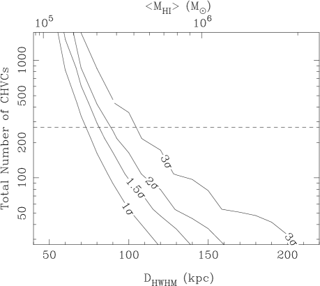
Figure 4.— Combined constraints on the Milky Way CHVC population as a function of the number of CHVCs per group and D_HWHM (or the average H I mass of the CHVC) assuming a three-dimensional Gaussian distance distribution. The dashed line marks the number of CHVCs identified around the Milky Way.

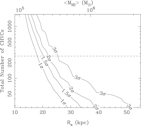
Figure 5.— As in Figure 4, but plotted as a function of $r_{s}$ for an NFW distribution.

Figure 6.— The H I mass function for Milky Way CHVCs with a Gaussian distance distribution with D${}_{HWHM}=90kpc$. The error bars reflect the standard deviation in each mass bin.

Figure 7.— The cumulative distance distribution of Milky Way satellites (solid line with stars), the Kravtsov et al. (2004) CDM subhalos (dotted line), and for a Gaussian distribution with D${}_{HWHM}=90kpc$ (solid line) and a NFW distribution with $r_{s}=22kpc$ (dashed line).

References

- Auld et al. (2006) Auld, R., et al. 2006, MNRAS, 953, in press
- Barbieri et al. (2005) Barbieri, C. V., Fraternali, F., Oosterloo, T., Bertin, G., Boomsma, R., & Sancisi, R. 2005, A&A, 439, 947
- Barnes et al. (2001) Barnes, D. G., et al. 2001, MNRAS, 322, 486
- Bekki et al. (2005a) Bekki, K., Koribalski, B. S., Ryder, S. D., & Couch, W. J. 2005, MNRAS, 357, L21
- Bekki et al. (2005b) Bekki, K., Koribalski, B. S., & Kilborn, V. A. 2005, MNRAS, 363, L21
- Blitz et al. (1999) Blitz, L., Spergel, D.N., Teuben, P.J., Hartmann, D., & Burton, W.B., 1999, ApJ, 514, 818
- de Blok et al. (2002) de Blok, W. J. G., Zwaan, M. A., Dijkstra, M., Briggs, F. H., & Freeman, K. C. 2002, A&A, 382, 43
- Boomsma et al. (2004) Boomsma, R., van der Hulst, T., Oosterloo, T., Fraternali, F., & Sancisi, R. 2004, IAU Symposium, 217, 142
- Boomsma et al. (2005) Boomsma, R., Oosterloo, T. A., Fraternali, F., van der Hulst, J. M., & Sancisi, R. 2005, A&A, 431, 65
- Braun & Burton (1999) Braun R., Burton W.B., 1999, A&A, 351, 437
- Braun & Thilker (2004) Braun, R., & Thilker, D. A. 2004, A&A, 417, 421
- Bravo-Alfaro et al. (2000) Bravo-Alfaro, H., Cayatte, V., van Gorkom, J. H., & Balkowski, C. 2000, AJ, 119, 580
- Bregman (1980) Bregman, J. N. 1980, ApJ, 236, 577
- Brüns et al. (2000) Brüns, C., Kerp, J., Kalberla, P. M. W., & Mebold, U. 2000, A&A, 357, 120
- Brüns et al. (2001) Brüns, C., Kerp, J., & Pagels, A. 2001, A&A, 370, L26
- Burns et al. (1994) Burns, J. O., Roettiger, K., Ledlow, M., & Klypin, A. 1994, ApJ, 427, L87
- Forbes et al. (2006) Forbes, D.A., et al. 2006, PASA, 23, 38
- Fraternali et al. (2002) Fraternali, F., van Moorsel, G., Sancisi, R., & Oosterloo, T. 2002, AJ, 123, 3124
- Freeman & Bland-Hawthorn (2002) Freeman, K., & Bland-Hawthorn, J. 2002, ARA&A, 40, 487
- Fukugita & Peebles (2006) Fukugita, M., & Peebles, P. J. E. 2006, ApJ, 639, 590
- Garcia (1993) Garcia, A.M., 1993, A&AS, 100, 47
- Gibson et al. (2001) Gibson, B. K., Giroux, M. L., Penton, S. V., Stocke, J. T., Shull, J. M., & Tumlinson, J. 2001, AJ, 122, 3280
- Giovanelli & Haynes (1989) Giovanelli, R., & Haynes, M. P. 1989, ApJ, 346, L5
- Gonzalez et al. (2005) Gonzalez, A. H., Tran, K.-V. H., Conbere, M. N., & Zaritsky, D. 2005, ApJ, 624, L73
- Grebel et al. (2003) Grebel, E. K., Gallagher, J. S., III, & Harbeck, D. 2003, AJ, 125, 1926
- de Heij et al. (2002a) de Heij V., Braun R., Burton W.B., 2002a, A&A, 391, 67
- de Heij et al. (2002b) de Heij V., Braun R., Burton W.B., 2002b, A&A, 392, 417
- Hibbard et al. (2001) Hibbard, J. E., van Gorkom, J. H., Rupen, M. P., & Schiminovich, D. 2001, ASP Conf. Ser. 240: Gas and Galaxy Evolution, 240, 657
- Hunter et al. (1998) Hunter, D. A., Wilcots, E. M., van Woerden, H., Gallagher, J. S., & Kohle, S. 1998, ApJ, 495, L47
- Kamphuis & Sancisi (1993) Kamphuis, J., & Sancisi, R. 1993, A&A, 273, L31
- Kaufmann et al. (2006) Kaufmann, T., Mayer, L., Wadsley, J., Stadel, J., & Moore, B. 2006, MNRAS, 370, 1612
- Kilborn et al. (2005) Kilborn, V.A., Koribalski, B.S., Forbes, D.A., Barnes, D.G., & Musgrave, R.C. 2005, MNRAS, 356, 77
- Kilborn et al. (2006) Kilborn, V.A., Forbes, D.A., Koribalski, B.S., Brough, S., & Kern, K. 2006, MNRAS, 371, 739
- Klypin et al. (1999) Klypin, A., Kravtsov, A.V., Valenzuela, O., & Prada, F., 1999, ApJ, 522, 82
- Klypin et al. (2002) Klypin, A., Zhao, H., & Somerville, R. S. 2002, ApJ, 573, 597
- Kovac̆ et al. (2005) Kovac̆, K., Oosterloo, T. A., & van der Hulst, J. M. 2005, IAU Colloq. 198: Near-fields cosmology with dwarf elliptical galaxies, 351
- Kraan-Korteweg et al. (1999) Kraan-Korteweg, R. C., van Driel, W., Briggs, F., Binggeli, B., & Mostefaoui, T. I. 1999, A&AS, 135, 255
- Kravtsov et al. (2004) Kravtsov, A. V., Gnedin, O. Y., & Klypin, A. A. 2004, ApJ, 609, 482
- Lo & Sargent (1979) Lo, K. Y., & Sargent, W. L. W. 1979, ApJ, 227, 756
- Lockman et al. (2002) Lockman, F. J., Murphy, E. M., Petty-Powell, S., & Urick, V. J. 2002, ApJS, 140, 331
- Lockman (2003) Lockman, F.J., 2003, ApJ, 591, L33
- Maller & Bullock (2004) Maller, A. H., & Bullock, J. S. 2004, MNRAS, 355, 694
- Maloney & Putman (2003) Maloney, P. R., & Putman, M. E. 2003, ApJ, 589, 270
- Masters (2005) Masters, K.L., 2005, Ph.D. Thesis, Cornell University
- Meyer et al. (2004) Meyer, M. J., et al. 2004, MNRAS, 350, 1195
- Miller & Bregman (2005) Miller, E. D., & Bregman, J. N. 2005, ASP Conf. Ser. 331: Extra-Planar Gas, 331, 261
- Minchin et al. (2003) Minchin, R. F., et al. 2003, MNRAS, 346, 787
- McMahon et al. (1990) McMahon, R. G., Irwin, M. J., Giovanelli, R., Haynes, M. P., Wolfe, A. M., & Hazard, C. 1990, ApJ, 359, 302
- Moore et al. (1999) Moore, B., Ghigna, S., Governato, F., Lake, G., Quinn, T., Stadel, J., & Tozzi, P., 1999, ApJ, 524, L19
- Muller et al. (1963) Muller, C.A., Oort,J.H., Raimond, E., 1963, C.R. Acad. Sci. Paris, 257, 1661
- Murphy et al. (1995) Murphy, E.M., Lockman, F.J., Savage, B.D., 1995, ApJ, 447, 624
- Navarro et al. (1996) Navarro, J. F., Frenk, C. S., & White, S. D. M. 1996, ApJ, 462, 563
- Navarro et al. (1997) Navarro, J. F., Frenk, C. S., & White, S. D. M. 1997, ApJ, 490, 493
- Nicastro et al. (2003) Nicastro, F., et al. 2003, Nature, 421, 719
- Oort (1966) Oort, J.H., 1966, BAN, 18, 421
- Oort (1970) Oort, J.H., 1970, A&A, 7, 381
- Pisano et al. (1998) Pisano, D. J., Wilcots, E. M., & Elmegreen, B. G. 1998, AJ, 115, 975
- Pisano et al. (2002) Pisano, D. J., Wilcots, E. M., & Liu, C. T. 2002, ApJS, 142, 161
- Pisano et al. (2004) Pisano, D. J., Barnes, D. G., Gibson, B. K., Staveley-Smith, L., Freeman, K. C., & Kilborn, V. A. 2004, ApJ, 610, L17 (Paper I)
- Pisano et al. (2006) Pisano, D. J., Barnes, D. G., Gibson, B. K., Staveley-Smith, L., Freeman, K. C., & Kilborn, V. A. 2007, in preparation (Paper III)
- Putman et al. (2002) Putman, M.E., et al., 2002, AJ, 123, 873
- Putman et al. (2003) Putman, M. E., Bland-Hawthorn, J., Veilleux, S., Gibson, B. K., Freeman, K. C., & Maloney, P. R. 2003, ApJ, 597, 948
- Putman et al. (2004) Putman, M.E., Thom, C., Gibson, B.K., Staveley-Smith, L., 2004, ApJ, 603, L77
- Putman (2006) Putman, M. E. 2006, ApJ, 645, 1164
- Quilis & Moore (2001) Quilis, V., & Moore, B. 2001, ApJ, 555, L95
- Ryder et al. (2001) Ryder, S. D., et al. 2001, ApJ, 555, 232
- Schneider et al. (1983) Schneider, S. E., Helou, G., Salpeter, E. E., & Terzian, Y. 1983, ApJ, 273, L1
- Schneider (1985) Schneider, S. 1985, ApJ, 288, L33
- Schulman et al. (1994) Schulman, E., Bregman, J. N., & Roberts, M. S. 1994, ApJ, 423, 180
- Sembach et al. (2003) Sembach, K. R., et al. 2003, ApJS, 146, 165
- Siegel et al. (2005) Siegel, M. H., Majewski, S. R., Gallart, C., Sohn, S. T., Kunkel, W. E., & Braun, R. 2005, ApJ, 623, 181
- Shapiro & Field (1976) Shapiro, P. R., & Field, G. B. 1976, ApJ, 205, 762
- Simon & Blitz (2002) Simon, J. D., & Blitz, L. 2002, ApJ, 574, 726
- Sommer-Larsen (2006) Sommer-Larsen, J. 2006, ApJ, 644, L1
- Spergel et al. (2003) Spergel, D. N., et al. 2003, ApJS, 148, 175
- Staveley-Smith et al. (1996) Staveley-Smith, L., et al. 1996, PASA, 13, 243
- Sternberg et al. (2002) Sternberg, A., McKee, C. F., & Wolfire, M. G. 2002, ApJS, 143, 419
- Stevens (2005) Stevens, J.B., 2005, Ph.D. thesis, Uni. Melboure
- Swaters et al. (1997) Swaters, R. A., Sancisi, R., & van der Hulst, J. M. 1997, ApJ, 491, 140
- Theis & Kohle (2001) Theis, C., & Kohle, S. 2001, A&A, 370, 365
- Thilker et al. (2004) Thilker, D. A., Braun, R., Walterbos, R. A. M., Corbelli, E., Lockman, F. J., Murphy, E., & Maddalena, R. 2004, ApJ, 601, L39
- Thom et al. (2006) Thom, C., Putman, M. E., Gibson, B. K., Christlieb, N., Flynn, C., Beers, T. C., Wilhelm, R., & Lee, Y. S. 2006, ApJ, 638, L97
- Tripp et al. (2000) Tripp, T. M., Savage, B. D., & Jenkins, E. B. 2000, ApJ, 534, L1
- Tripp & Savage (2000) Tripp, T. M., & Savage, B. D. 2000, ApJ, 542, 42
- Tripp et al. (2003) Tripp, T. M., et al. 2003, AJ, 125, 3122
- Tufte et al. (2002) Tufte, S. L., Wilson, J. D., Madsen, G. J., Haffner, L. M., & Reynolds, R. J. 2002, ApJ, 572, L153
- Tully (1987) Tully, R.B., 1987, ApJ, 321, 280
- Wakker & van Woerden (1997) Wakker, B.P., & van Woerden, H., 1997, ARA&A, 35, 217
- Wakker et al. (1999) Wakker, B. P., et al. 1999, Nature, 402, 388
- Wakker (2001) Wakker, B. P. 2001, ApJS, 136, 463
- Wakker et al. (2003) Wakker, B. P., et al. 2003, ApJS, 146, 1
- Weiner (2003) Weiner, B. J. 2003, ASSL Vol. 281: The IGM/Galaxy Connection. The Distribution of Baryons at z=0, 163
- Westmeier et al. (2005) Westmeier, T., Brüns, C., & Kerp, J. 2005, A&A, 432, 937
- Westmeier et al. (2005) Westmeier, T., Braun, R., Bruens, C., Kerp, J., & Thilker, D. 2005, Astronomische Nachrichten, 326, 520
- White & Frenk (1991) White, S. D. M., & Frenk, C. S. 1991, ApJ, 379, 52
- White & Rees (1978) White, S. D. M., & Rees, M. J. 1978, MNRAS, 183, 341
- Wilcots et al. (1996) Wilcots, E. M., Lehman, C., & Miller, B. 1996, AJ, 111, 1575
- Wilcots & Miller (1998) Wilcots, E. M., & Miller, B. W. 1998, AJ, 116, 2363
- Wilcots & Prescott (2004) Wilcots, E. M., & Prescott, M. K. M. 2004, AJ, 127, 1900
- Willman et al. (2002) Willman, B., Dalcanton, J., Ivezić, Ž., Schneider, D. P., & York, D. G. 2002, AJ, 124, 2600
- van Woerden et al. (1999) van Woerden, H., Schwarz, U. J., Peletier, R. F., Wakker, B. P., & Kalberla, P. M. W. 1999, Nature, 400, 138
- van Woerden et al (2004) van Woerden, H., Wakker, B. P., Schwarz, U. J., & de Boer, K. S., eds., 2004, High Velocity Clouds. ASTROPHYSICS AND SPACE SCIENCE LIBRARY Volume 312. Kluwer Academic Publishers, Dordrecht.
- Zabludoff & Mulchaey (1998) Zabludoff, A.I., & Mulchaey, J.S., 1998, ApJ, 498, L5
- Zwaan & Briggs (2000) Zwaan, M. A., & Briggs, F. H. 2000, ApJ, 530, L61
- Zwaan (2001) Zwaan, M. A. 2001, MNRAS, 325, 1142
- Zwaan et al. (2004) Zwaan, M. A., et al. 2004, MNRAS, 350, 1210