Cross-correlation in four dimensions: Application to the quadruple-lined spectroscopic system HD 110555

Abstract

We develop a technique to measure radial velocities of stars from spectra that present four sets of lines. The algorithm is an extension of the two-dimensional cross-correlation method TODCOR to four dimensions. It computes the correlation of the observed spectrum against a combination of four templates with all possible shifts, and allows also for the derivation of the light ratios of the components. After testing the algorithm and demonstrating its ability to measure Doppler shifts accurately even under conditions of heavy line blending, we apply it to the case of the quadruple-lined system HD 110555. The primary and secondary components of this previously known visual binary ($\rho\sim 0\farcs 4$) are each shown to be double-lined spectroscopic binaries with periods of 57 days and 76 days, respectively, making the system a hierarchical quadruple. The secondary in the 76-day subsystem contributes only 2.5% to the total light, illustrating the ability of the method to measure velocities of very faint components.

1. Introduction

The use of digital cross-correlation as an analysis tool in spectroscopy dates back at least three decades. Early applications by Simkin (1974), Lacy (1977), Tonry & Davis (1979), and others, showed the power of the method for measuring accurate radial velocities, and with many improvements and refinements over the years the technique enjoys widespread use today (for further details and a historical perspective see, e.g., Hill, 1993; Kurtz & Mink, 1998). Compared to the classical method of measuring the positions of individual spectral lines (still occasionally used), cross-correlation offers a number of important advantages beyond expediency, principally its ability to make efficient use of all the information available in the spectral window. It is thus ideal for the analysis of low signal-to-noise spectra, where classical methods tend to give poorer results. It is also commonly used on composite spectra, e.g., double-lined spectroscopic binaries, where the Doppler shifts are typically determined from the centroids of the two correlation peaks that correspond to the each of the components of the binary. Difficulties arise, however, when the peaks are not well separated, and this can lead to systematic errors in the radial velocities that bias the amplitudes of the velocity curves and any physical quantities derived from them (such as the masses), or it can prevent the measurement altogether.

To address this problem Zucker & Mazeh (1994) developed an extension of the standard one-dimensional cross-correlation technique to two dimensions (TODCOR), taking advantage of the properties of the Fourier transform. TODCOR uses two templates, one for each component of the binary, and thus the cross-correlation function (CCF) now depends on the velocities of both stars relative to their templates. The location of the maximum in two-dimensional velocity space corresponds to the Doppler shifts of the two components. This effectively decouples the primary from the secondary so that, if the templates are a good match to the stars, blending between them is no longer a concern. A further extension of TODCOR to three dimensions was subsequently introduced by Zucker et al. (1995) to deal with triple-lined spectra, in which line blending is usually more common. In this case the standard one-dimensional CCF would in principle reveal three peaks (at favorable orbital phases), but the difficulties of measuring their centroids by classical means can be even greater than in the double-lined case. The success of the three-dimensional version of TODCOR to overcome these difficulties is illustrated by a number of applications over the last decade since its introduction (Torres et al., 1995; Jha et al., 2000; Mazeh et al., 2001; Covino et al., 2001; Torres et al., 2002, 2006).

A recent study by Tokovinin et al. (2006) has shown that spectroscopic binaries of solar-type are very often accompanied by more distant components. The frequency of such multiple systems appears to be very high: up to 97% of spectroscopic binaries with periods shorter than 3 days show at least one additional companion, tapering off to 34% for periods longer than 12 days (see Fig. 14 by Tokovinin et al., 2006). Out of the 161 systems in their sample, 64 were found to be triple and 11 were found to be quadruple. Thus the frequency of systems with four stars is not negligible, and it is to be expected that some fraction of them will show lines of all four stars in the spectra, although they may not always be easy to recognize. These will typically be hierarchical quadruple systems composed of two relatively tight binaries in a wide orbit around each other, with an angular separation of order an arc second or less so that they are unresolved at the spectrograph slit (or optical fiber entrance). The ability to measure the radial velocities of the 4 stars in these systems is essential for deriving properties such as their masses, as well as other orbital characteristics, and these in turn are important for understanding the origin and evolution of multiple systems in general, and higher multiplicity systems in particular.

The extensive spectroscopic surveys at the Harvard-Smithsonian Center for Astrophysics (CfA) with the CfA Digital Speedometers (Latham, 1992) have revealed an appreciable number of triple-lined systems, and indeed even some cases with four sets of lines that have until now remained unsolved because of the complexity of the analysis and our concerns about blending. This provides the motivation for the present work, in which we develop an extension of TODCOR to four dimensions, allowing the treatment of such cases. We demonstrate the effectiveness of the method with numerical simulations, showing that it is possible to measure the velocities of the four stars even in situations with severe line blending that would be hopeless using standard one-dimensional cross-correlation techniques. We then apply the method to the real case of HD 110555, which enabled us to detect for the first time the very faint 4th component and to measure its Doppler shift, in addition to obtaining the relative brightnesses of the stars.

2. Description of the method

TODCOR as introduced by Zucker & Mazeh (1994) is a two-dimensional cross-correlation scheme in which the observed spectra, $f(n)$, are cross-correlated against a composite template, $g(n)$, that is the sum of two separate templates selected to match the properties of each of the binary components. The template $g$ for this two-dimensional case is given by $g=g_{1}(n-s_{1})+\alpha\ g_{2}(n-s_{2})$, where $s_{1}$ and $s_{2}$ represent the shifts of the individual templates ($g_{1}$ and $g_{2}$) needed to match the true Doppler shift of the respective component. The coefficient $\alpha$ is the light ratio between the secondary and the primary, which is assumed initially to be known. The cross-correlation between $f$ and $g$ is performed for all possible shifts of the two templates, and the resulting function of $s_{1}$ and $s_{2}$ will typically have a global maximum, the location of which provides the Doppler shifts of both stars. Brute-force computation of these cross-correlations over all possible shifts is impractical. However, Zucker & Mazeh (1994) showed that the two-dimensional correlation function $\mathcal{R}^{(2)}=\mathcal{R}^{(2)}(s_{1},s_{2})$ can be expressed analytically in terms of three one-dimensional correlation functions which are much more economical to compute. As they pointed out, computing one-dimensional CCFs is an $\mathcal{O}(N^{2})$ process, where $N$ is the number of pixels in $f$, but by using the properties of Fourier transforms the problem can be reduced to an $\mathcal{O}(N\log N)$ process. This reduction in the number of operations required is preserved in $\mathcal{R}^{(2)}$, and is what makes the method practical. In the more general case in which the light ratio is unknown, the correlation function $\mathcal{R}^{(2)}$ also depends on $\alpha$, or $\mathcal{R}^{(2)}=\mathcal{R}^{(2)}(s_{1},s_{2},\alpha)$. An analytical expression can be found for $\alpha$ that maximizes the correlation for each pair of shifts $s_{1}$ and $s_{2}$, and this expression depends on the same three one-dimensional CCFs (see Zucker & Mazeh, 1994).

The extension of TODCOR to three dimensions presented by Zucker et al. (1995) is fairly straightforward, the algebra being somewhat more involved. The Fourier transform properties once again reduce the computational problem to an $\mathcal{O}(N\log N)$ process. Conceptually it is just as straightforward to extend the scheme to four dimensions for the analysis of quadruple-lined spectroscopic systems, although the algebra in this case is considerably more complex. The template is now assumed to be a combination of four separate (i.e., possibly different) templates, each with its own shift, and three light ratios:

$$g=g_{1}(n-s_{1})+\alpha\ g_{2}(n-s_{2})+\beta\ g_{3}(n-s_{3})+\gamma\ g_{4}(n-s_{4})~{},$$

where $\beta$ and $\gamma$ are the light ratio of the tertiary and quaternary components relative to the primary. The four-dimensional CCF for the case in which the light ratios are known, $\mathcal{R}^{(4)}=\mathcal{R}^{(4)}(s_{1},s_{2},s_{3},s_{4})$, can again be expressed analytically in terms of one-dimensional correlation functions and three light ratios, as described in the Appendix. These one-dimensional correlations are between the observed spectrum and each of the four templates, as well as between pairs of templates (in all combinations). To determine the velocities of the four stars one simply searches for the maximum of $\mathcal{R}^{(4)}$ in the four-dimensional space of $\{s_{1},s_{2},s_{3},s_{4}\}$. For the more likely case in which the light ratios are unknown to begin with, analytical expressions can be found for $\alpha$, $\beta$, and $\gamma$ in terms of the same one-dimensional CCFs mentioned above (see Appendix). These values can then be inserted into the expression for $\mathcal{R}^{(4)}$. Thus the method is completely general in that it permits in principle the determination of all unknown quantities directly from the observed spectra. The only requirement is that the four templates chosen for the cross-correlations be a reasonably good match to each of the components of the quadruple system.

3. Testing the algorithm

In order to test the method we generated synthetic composite spectra to simulate observations of a quadruple-lined system by adding together four calculated spectra with various relative shifts and intensity ratios. Those same four calculated spectra were in turn used as individual templates ($g_{1},g_{2},g_{3},g_{4}$) in our four-dimensional extension of TODCOR. All synthetic spectra were taken from a large library of calculated spectra created by Jon Morse (see also Nordström et al., 1994; Latham et al., 2002), based on model atmospheres by R. L. Kurucz, which we also use in the next section to analyze a real case. These spectra cover a wavelength range of approximately 80 Å centered at 5187 Å, and have a resolving power of $\lambda/\Delta\lambda\approx 35,\!000$. They were intended for use with spectroscopic observations obtained with the CfA Digital Speedometers, which have a narrower wavelength coverage of only 45 Å, so for comparison purposes we have considered only this reduced spectral window in our tests. Furthermore, in order to make the simulations more realistic we have added Poisson noise corresponding to different signal-to-noise ratios (SNR).

As a first example among the many experiments we carried out, we consider a case with the relative shifts of the four individual stars selected to demonstrate the ability of the algorithm to measure velocities under conditions of significant line blending. Our simulated quadruple system in this case is composed of non-rotating stars of spectral types G0V, G2V, G0V, and G2V for the primary, secondary, tertiary, and quaternary, respectively, corresponding to effective temperatures ($T_{\rm eff}$) for the templates of 6000 K, 5750 K, 6000 K, and 5750 K. The templates were added together (initially with no noise) with Doppler shifts of $+20~{}{\rm km\thinspace s^{-1}}$, $-20~{}{\rm km\thinspace s^{-1}}$, $+10~{}{\rm km\thinspace s^{-1}}$, and $-5~{}{\rm km\thinspace s^{-1}}$, respectively, and with intensity ratios of $\alpha=0.50$ (secondary/primary), $\beta=0.80$ (tertiary/primary), and $\gamma=0.50$ (quaternary/primary). Although some signs of the composite nature of this artificial spectrum can be seen by careful visual comparison with the primary template, it is not possible to identify the lines of the four components, and this would only worsen in the presence of noise. The top panel of Figure 1 shows the standard one-dimensional CCF we obtain by correlating the above noiseless synthetic composite spectrum against the primary template. This and all other one-dimensional CCFs in this paper are computed using the IRAF task XCSAO (Kurtz & Mink, 1998). The input velocities of each component are indicated in the figure with vertical dotted lines. The blending of the correlation peaks is such that the velocities of the individual stars are not measurable in this case with standard techniques. Application of the four-dimensional cross-correlation technique, on the other hand, is able to recover the four velocities as well as the light ratios reliably. To show this quantitatively and to provide at the same time a realistic measure of the uncertainty due to noise, we have added Poisson noise to the input composite spectrum corresponding to a SNR = 25, and generated 50 quadruple-lined spectra with different noise but with the same shifts. We then processed these spectra as described above. The results are shown in Table 1 (middle section under “Test 1”), where we list the mean velocities obtained for each star from the 50 spectra, as well as the mean light ratios. The uncertainties attached to these means are simply the scatter of the 50 values, so they represent the typical error for a determination from a single spectrum. Both the input velocities and the input light ratios are recovered to well within their errors, showing the power of the technique in this very demanding case. Cross-sections of the four-dimensional CCF for the case of no noise are shown in the lower panels of Figure 1. For example, the second panel shows a cut along the velocity axis corresponding to the primary star, with the velocities of the other three components held fixed at the values that maximize the correlation function. A peak is clearly seen precisely at the location of the input value for the velocity of that star (dotted line). Similarly, cross-sections for each of the other components show a prominent peak at the correct velocity.

As a second test we reduced the SNR to 10 and repeated the velocity and light ratio determinations for the 50 simulated spectra (see Table 1, “Test 2”). In this case the velocities are typically still recovered quite reliably (within a few km s^-1), and although the mean values of $\alpha$, $\beta$, and $\gamma$ are also not far from their input values, their scatter is much larger. However, as stated above this scatter represents the typical error for a single measurement. In a real application there will in general be multiple spectra of the object, so if the light ratios are constant one can hope for a $\sqrt{N}$ gain in taking the averages.

A third experiment was carried out in which we examined the ability of the algorithm to recover faint components in quadruple-lined spectra. For this test we adopted templates corresponding to spectral types G0V, G2V, G2V, and K4V (temperatures of 6000 K, 5750 K, 5750 K, and 4750 K), and we relaxed the line blending by adopting somewhat larger Doppler shifts of $+50~{}{\rm km\thinspace s^{-1}}$, $-50~{}{\rm km\thinspace s^{-1}}$, $+20~{}{\rm km\thinspace s^{-1}}$, and $-20~{}{\rm km\thinspace s^{-1}}$. The SNR was set to 50 in this case, and we chose $\alpha=0.70$ and $\beta=0.60$. For $\gamma$ we tested a range of values from 0.20 to 0.01, and we found that the correct velocities were always recovered reliably by the algorithm for the primary, secondary, and tertiary components, and that the input values of $\alpha$ and $\beta$ were recovered as well. The velocities for the fourth star deteriorated with decreasing $\gamma$, as expected, but were still measurable down to $\gamma=0.03$ ($s_{4}=-22.4\pm 1.9$ km s^-1 for the mean of 50 trials). At this light ratio the recovered value of $\gamma$ was $0.039\pm 0.004$, which is slightly overestimated. At a lower light ratio of 2% the fourth star was only detectable in about half of these artificial spectra.

The above tests and many others we carried out show that the algorithm performs well under conditions of severe line blending allowing the reliable determination of radial velocities, and also demonstrate its ability to detect faint components in quadruple-lined spectra. It is clear that the sensitivity to faint companions depends strongly on the degree of line blending of the component in question, as well as on the SNR of the spectra. In the next section we apply the method to a real case. The performance of the algorithm will usually depend also on how closely the four templates represent the individual stars. In the experiments in this section the templates we have used are, by construction, a perfect match to the components. The effects of mismatch have not been addressed here because they depend on the properties of the particular system under investigation, and it is difficult to make general statements that are useful in a different case. We discuss this further in §5.

4. Application to HD 110555

The relatively bright star HD 110555 (also known as BD+06 2647, HIP 62034, and ADS 8639 AB, $\alpha=12^{\rm h}42^{\rm m}55\fs 36$, $\delta=+05\arcdeg 15\arcmin 59\farcs 1$, J2000, spectral type G5, $V=8.36$) is a close ($\rho\sim 0\farcs 4$) visual binary discovered by R. G. Aitken at the Lick Observatory in 1907 (Aitken, 1908). It was observed spectroscopically at the CfA as part of a large sample of G dwarfs that have been monitored for more than 15 years. In the course of that project we obtained a total of 48 usable spectra of HD 110555 between 1993 January and 2004 March, mostly with an echelle spectrograph mounted on the 1.5m Wyeth reflector at the Oak Ridge Observatory (Harvard, Massachusetts). A single echelle order spanning 45 Å was recorded with a photon-counting Reticon diode array at a mean wavelength of 5188.5 Å, which includes the Mg I b triplet. The SNRs of these observations range from about 11 to 42 per resolution element of 8.5 km s^-1. Two of the spectra were obtained with a nearly identical setup using the 1.5m Tillinghast reflector at the F. L. Whipple Observatory (Mount Hopkins, Arizona). Because of the close separation of the binary and the 1″ width of the spectrograph slit, the system was observed as a single object. The zero-point of the velocity scale was monitored by means of exposures of the dusk and dawn sky, and small run-to-run corrections were applied to the velocities derived below in the manner described by Stefanik et al. (1999).

The first few spectra of HD 110555 showed obvious signs of at least two sets of lines separated in velocity by as much as 80 km s^-1, which, in view of the small angular separation of the visual pair, suggested that at least one of the visual components is a spectroscopic binary with a relatively short period. Figure 2 includes a small sampling of our observations showing the spectra and one-dimensional CCFs computed using a template corresponding to a G0 star. Some of the observations even showed three sets of lines, and the appearance of the correlation functions varied on a timescale of a week or so. Changes in velocity had not previously been measured for HD 110555, and in fact we are only aware of a single velocity measurement in the literature reported by Nordström et al. (2004) yielding $RV=-40.9\pm 0.8$ km s^-1, which is, however, unlikely to be very meaningful in view of the complicated nature of the system.

Preliminary velocity determinations were carried out initially using the two-dimensional version of TODCOR, focusing on the two dominant correlation peaks, and later with the three-dimensional version of the algorithm to account for the third peak. For these analyses we adopted solar-type templates for all stars ($T_{\rm eff}=5750$ K), with no rotational broadening since the composite spectra do not exhibit significant line broadening at phases where the lines are all blended. The surface gravity was set to $\log g=4.5$, as appropriate for dwarfs, and solar composition was assumed. The results showed that the system is composed of a double-lined binary with a period of about 57 days, and a single-lined binary with a period of $\sim$76 days. No sign of the secondary of the latter system was apparent. The preliminary center-of-mass velocities of these orbits were within a few km s^-1 of each other, indicating the physical association of the two binaries and leading us to conclude that they most likely correspond to each of the components of the visual binary. The HD 110555 system is therefore a hierarchical quadruple.

We then applied our new algorithm in an attempt to detect the fourth star (secondary of the 76-day binary) and measure its velocity. The template adopted in this case was somewhat cooler ($T_{\rm eff}=5000$ K). All 48 of our spectra showed evidence of a weak set of lines at approximately the expected location. An example is shown in Figure 3, which corresponds to the same spectrum displayed in the bottom panel of Figure 2, in which the three brighter components are quite heavily blended. The top panel of Figure 3 shows the one-dimensional CCF once again, only on an expanded scale, and the lower four panels show cuts of the four-dimensional CCF along the axes corresponding to each of the components, as in Figure 1. We indicate with vertical dotted lines the predicted velocities from our final spectroscopic orbits, described below. The cross-section for the quaternary is noisy, but it does present a peak at the expected location, and the same is true for each of our other spectra.

The preliminary light ratios we derived clearly indicated that the 57-day binary is brighter than the 76-day binary, so it must correspond to the visual primary. We refer to this system as “A”, composed of stars Aa and Ab, following the usual spectroscopic notation. Similar designations are adopted for the visual secondary, “B”. In order to fine-tune the templates for the four stars we made use of model isochrones from the Padova series by Girardi et al. (2000), combined with all available observational constraints. These include, in addition to the three preliminary light ratios, the combined $B\!-\!V$ color of the quadruple system as listed in the Hipparcos Catalogue (ESA, 1997), the $V\!-\!J$, $V\!-\!H$, and $V\!-\!K$ indices derived from the Johnson $V$ magnitude (Hipparcos) and 2MASS Catalog (Skrutskie et al., 2006), properly converted to the same photometric system as the stellar models (Carpenter, 2001), the magnitude difference of the visual pair ($\Delta V$) as measured by Hipparcos and converted to the visual band following Harmanec (1998), and the preliminary mass ratios for the two spectroscopic binaries. By requiring simultaneous agreement with all observational quantities we were able to select four stars from a representative model isochrone of solar metallicity and age 3 Gyr that yield a consistent picture of the system, and allow us to read off the effective temperatures as well as other theoretical properties. The temperatures were close to 6000 K for Aa and Ab, 5500 K for Ba, and 4750 K for the fainter component Bb, which are the nearest values in our library of synthetic spectra. The surface gravities were not far from $\log g=4.5$, as expected for dwarfs, supporting our earlier choice of this value. The fairly close agreement between all observational constraints and the results from the model is shown in Table 2, where the differences in the last column are seen to be of order 1.3$\sigma$ or less. The inferred properties of the four stars are listed in Table 3. They are unevolved dwarfs, so the stellar characteristics are quite insensitive to age for our purposes. Their location in the H-R diagram is illustrated in Figure 4. Templates with the above parameters and zero rotational broadening were then used to derive improved radial velocities, and the light ratios and mass ratios also changed slightly. One more iteration was sufficient to reach convergence on the temperature determination for the templates, given the relatively coarse 250 K step in our library of synthetic spectra. The final velocities were derived with the above template parameters, and the light ratios obtained were $\alpha=0.92$, $\beta=0.38$, and $\gamma=0.06$, determined as described in the Appendix. Uncertainties for these ratios are estimated to be about 0.03.

We present the velocities for the visual primary and visual secondary components in Table 4 and Table 5. The uncertainties ($\sigma$) associated with these measurements reflect both the SNR of each spectrum and the relative brightness of each component. They were derived as a byproduct of the orbital solutions, by assigning initial weights to the observations proportional to the strength of each exposure, and then scaling these initial errors so that the reduced $\chi^{2}$ values are near unity separately for the primary and secondary in each subsystem. The orbital elements we obtain for the two spectroscopic binaries are listed in Table 6. They are the period ($P$), center-of-mass velocity ($V_{0}$), velocity semi-amplitudes ($K_{\rm prim},K_{\rm sec}$), eccentricity ($e$), longitude of periastron for the primary ($\omega_{\rm prim}$), and the time of periastron passage ($T$). Derived quantities of interest are listed as well (minimum masses, mass ratio, and projected semimajor axes). The velocity measurements in these fits have been weighted in the usual way according to their uncertainties. The rms residuals of the fit for star Ba ($\sim$1.7 km s^-1) and especially Bb ($\sim$5.4 km s^-1) are considerably larger than those of Aa and Ab ($\sim$0.7 km s^-1) on account of their faintness, which represents only about 16% and 2.5% of the total brightness of the system at this wavelength. Stars Aa and Ab contribute 42.5% and 39% to the total light. The velocity measurements and corresponding orbital fits are shown graphically in Figure 5.

A visual orbit determination for HD 110555 A and B has been published by Ling (2004) with a period of $1263\pm 125$ yr, an angular semimajor axis of $1\farcs 915\pm 0\farcs 022$ (corresponding to $\sim$150 AU), and a very large eccentricity of $e=0.983\pm 0.001$. However, due to the small number of measurements and their coverage of only a fraction of the orbit, it is assigned “Grade 5” (“indeterminate”) in the Sixth Catalog of Orbits of Visual Binary Stars maintained at the USNO (Hartkopf et al., 2001), and must be regarded as very preliminary. Based on this solution Ling (2004) reported a dynamical mass for the system of 2.28 M_☉, which is, however, smaller than the sum of the minimum masses of the four stars from our spectroscopic orbits ($3.44\pm 0.07$ M_☉; Table 6). The total mass inferred from our modeling is 3.8 M_☉ (Table 3). It is quite possible that the visual elements can in fact be improved by imposing our total mass as a constraint. A further constraint is provided by our radial velocities of A and B. They span only 11 yr, and we see no trend in the residuals that would reflect motion in the outer orbit, but the difference in the center-of-mass velocities of the two spectroscopic binary orbits, $V_{0}(B)-V_{0}(A)=-0.26\pm 0.23$ km s^-1 (Table 6), provides information that is orthogonal to the astrometry, and is thus potentially very important. We note, finally, that as a result of our isochrone fitting described above, the inclination angles of the two spectroscopic binaries are inferred to be $\sim$72° (visual primary) and $\sim$81° (visual secondary), with uncertainties of roughly 5°. The inclination reported for the visual orbit is rather similar ($85\arcdeg$).

5. Discussion

The cross-correlation technique described and tested in this paper, which is an extension of the two-dimensional algorithm TODCOR, provides a conceptually simple and elegant way of deriving reliable radial velocities from stellar spectra in which four sets of lines are present. It may be thought of as a prescription for cross-correlating the observed spectra against a composite template made of the combination of four individual templates (one for each component) with all possible shifts. The ability to make use of four templates selected to match the properties of each star is one of the great strengths of the method. Standard one-dimensional cross-correlation methods use a single template, which may be a good representation of one of the stars but will in general not match the others as well. Thus the correlation will never be optimal. Another strength of our four-dimensional algorithm is its ability to produce good results even with low SNR spectra, as illustrated by the example of HD 110555, in which the SNRs are as low as 11. Even in weak spectra such as these we were able to measure the velocity of the faint fourth component that contributes only 2.5% to the light of the system (6% of the light of the primary), despite seeing no sign of it either in the original spectra or in the standard one-dimensional CCFs. The method has shown to be very effective as well in dealing with line blending, yielding accurate radial velocities for HD 110555 although the line separation between two or more of the components is sometimes as small as a few km s^-1.

Only a handful of examples of quadruple-lined spectroscopic systems have appeared previously in the literature in which reliable radial velocities were derived for all four stars. To our knowledge these are XY Leo (Barden, 1987), HD 221264 (Willmitch & Fekel, 1990), ET Boo, VW LMi, and TV UMi (Pribulla et al., 2006), AO Vel (González et al., 2006), and HD 30869 (Tomkin et al., 2007), all of which contain an eclipsing pair except for the second and last cases. A number of other spectroscopic quadruples have been identified (e.g., Pribulla & Rucinski, 2006), although velocity measurements have not yet been published and it is unclear whether these systems show four sets of lines. The material available to the authors of the studies mentioned above was generally of much higher quality than that employed here, with SNRs typically in the range of 100–150. The techniques employed to derive the velocities have varied considerably. In the case of XY Leo and HD 30869 the centroids of absorption lines were measured directly, or the observed spectra were fitted in a $\chi^{2}$ sense by coadding spectra of comparison stars appropriately shifted in velocity, rotationally broadened, and scaled in flux. In HD 221264 the lines of the four components were separated enough that they could be isolated, and radial velocities were derived by focusing on a set of unblended lines of one star at a time using one-dimensional cross-correlation methods restricted to the appropriate wavelength intervals. For ET Boo, VW LMi, and TV UMi the authors used the broadening function (BF) formalism developed by Rucinski (2002), which reduces the severity of blending compared to the one-dimensional cross-correlation technique. The peaks in the BFs for these systems were fitted using either Gaussian profiles or rotational profiles. Finally, for AO Vel an iterative scheme was used in which the disentangled spectra of the components and their Doppler shifts were computed in steps (see González & Levato, 2006). All of these obviously represent useful alternatives to the technique developed in this paper.

The advantages or disadvantages of each these methods generally depend on the particular case under consideration, and their ability to derive accurate radial velocities is a strong function of the degree of line blending, the relative brightness of the components, and the quality of the spectroscopic material, among other factors. As demonstrated with the experiments in §3 the four-dimensional extension of TODCOR presented here fares very well even when the spectra have relatively low SNR. Other procedures that have been developed more specifically for disentangling the spectra of multiple systems can also derive the Doppler shifts, such as the method by Simon & Sturm (1994) that works in wavelength space, and that of Hadrava (1995) in Fourier space, although we have not yet seen an application to quadruple-lined spectra.

An implicit requirement of the method developed in this paper is that the four templates present a close match to the individual spectra of the components. In our experience with the use of synthetic templates the most important parameters are the effective temperature and the rotational broadening. Template mismatch is a well known issue in digital cross-correlation that can result in biases in the radial velocities (see, e.g., Griffin et al., 2000). Similar concerns hold in the four-dimensional case (as in the two- and three-dimensional versions of TODCOR). Therefore, selection of the optimal templates must be done with care. It is possible in many cases to determine the template parameters from the observed spectra themselves, if the SNR is sufficient. Illustrations of this for the two- and three-dimensional versions are given by Torres et al. (2002) and Torres et al. (2006). The present example of HD 110555 does not lend itself to these determinations because of the faint fourth component, which is why we resorted to the use of models. Another possibility is to combine our method with one of the disentangling techniques, which should be able to produce separate spectra for each of the components that will have higher SNRs than any of the individual spectra. These could then be used as templates for the four-dimensional cross-correlation scheme in order to derive the velocities. While this would seem to be a rather obvious and elegant approach, it requires testing to determine the sensitivity of the velocities to the details of the disentangling.

$$\mathcal{R}^{(1)}(s)={\sum f(n)g(n-s)\over N\sigma_{f}\sigma_{g}}~{},$$ (1)

in which $N$ is the number of bins in the observed spectrum, $\sigma_{f}$ and $\sigma_{g}$ are the intensity standard deviations of the object and template spectra given by

$$\sigma_{f}^{2}={1\over N}\sum f(n)^{2}~{}~{},~{}~{}\sigma_{g}^{2}={1\over N}\sum g(n)^{2}~{},$$

and $s$ is the shift between the two. As is well known, the use of the Fast Fourier Transform (FFT) allows for a very efficient calculation of the numerator of eq.(1), which is what makes the cross-correlation method practical. This same property is key to the success of TODCOR and its extensions.

We now consider the template $g$ to be a linear combination of four separate templates, one for each star, with coefficients $\alpha$, $\beta$, and $\gamma$ being the light ratios of the secondary, tertiary, and quaternary components relative to the primary:

$$g=g_{1}(n-s_{1})+\alpha\ g_{2}(n-s_{2})+\beta\ g_{3}(n-s_{3})+\gamma\ g_{4}(n-s_{4})~{}.$$

Substitution in eq.(1) yields

$$\mathcal{R}^{(4)}={\sum f(n)\ [g_{1}(n-s_{1})+\alpha\ g_{2}(n-s_{2})+\beta\ g_{3}(n-s_{3})+\gamma\ g_{4}(n-s_{4})]\over N\sigma_{f}\sigma_{g}(s_{1},s_{2},s_{3},s_{4})}~{},$$ (2)

in which

$$\sigma_{g}^{2}(s_{1},s_{2},s_{3},s_{4})={1\over N}\sum[g_{1}(n-s_{1})+\alpha\ g_{2}(n-s_{2})+\beta\ g_{3}(n-s_{3})+\gamma\ g_{4}(n-s_{4})]^{2}~{}.$$

The numerator of eq.(2) can be computed efficiently using FFT, since the four terms have the same form as eq.(1). The standard deviation $\sigma_{g}(s_{1},s_{2},s_{3},s_{4})$ in the denominator is

$$\sigma_{g}^{2}=\sigma^{2}_{g_{1}}+\alpha^{2}\sigma^{2}_{g_{2}}+\beta^{2}\sigma^{2}_{g_{3}}+\gamma^{2}\sigma^{2}_{g_{4}}+2\alpha\sigma_{12}+2\beta\sigma_{13}+2\gamma\sigma_{14}+2\alpha\beta\sigma_{23}+2\alpha\gamma\sigma_{24}+2\beta\gamma\sigma_{34}~{},$$ (3)

where we have defined, as in Zucker et al. (1995),

$$\sigma_{ij}(s_{j}-s_{i})\equiv{1\over N}\sum g_{i}(n-s_{i})g_{j}(n-s_{j})~{}.$$

The first four terms on the right-hand side of eq.(3) include the standard deviations of the templates. The other six terms have again the same form as the numerator in eq.(1), so they can be computed easily using FFT. If we now adopt the following additional definitions

$$C_{i}(s_{i}) \equiv {1\over N\sigma_{f}\sigma_{g_{i}}}\sum f(n)g_{i}(n-s_{i})$$ (4)

$$C_{ij}(s_{j}-s_{i}) \equiv {1\over N\sigma_{g_{i}}\sigma_{g_{j}}}\sum g_{i}(n)g_{j}\left[n-(s_{j}-s_{i})\right]~{},$$ (5)

we may write

$$\sigma_{g}^{2} = \sigma^{2}_{g_{1}}+\alpha^{2}\sigma^{2}_{g_{2}}+\beta^{2}\sigma^{2}_{g_{3}}+\gamma^{2}\sigma^{2}_{g_{4}}+2(\alpha\sigma_{g_{1}}\sigma_{g_{2}}C_{12}+\beta\sigma_{g_{1}}\sigma_{g_{3}}C_{13}+$$

$$\gamma\sigma_{g_{1}}\sigma_{g_{4}}C_{14}+\alpha\beta\sigma_{g_{2}}\sigma_{g_{3}}C_{23}+\alpha\gamma\sigma_{g_{2}}\sigma_{g_{4}}C_{24}+\beta\gamma\sigma_{g_{3}}\sigma_{g_{4}}C_{34})~{},$$

or

$$\sigma_{g}^{2}=\sigma^{2}_{g_{1}}\left[1+\alpha^{\prime 2}+\beta^{\prime 2}+\gamma^{\prime 2}+2(\alpha^{\prime}C_{12}+\beta^{\prime}C_{13}+\gamma^{\prime}C_{14}+\alpha^{\prime}\beta^{\prime}C_{23}+\alpha^{\prime}\gamma^{\prime}C_{24}+\beta^{\prime}\gamma^{\prime}C_{34})\right]~{},$$

where $\alpha^{\prime}\equiv\alpha(\sigma_{g_{2}}/\sigma_{g_{1}})$, $\beta^{\prime}\equiv\beta(\sigma_{g_{3}}/\sigma_{g_{1}})$, and $\gamma^{\prime}\equiv\gamma(\sigma_{g_{4}}/\sigma_{g_{1}})$. After some algebra the final expression for the four-dimensional CCF becomes

$$\mathcal{R}^{(4)}={C_{1}+\alpha^{\prime}C_{2}+\beta^{\prime}C_{3}+\gamma^{\prime}C_{4}\over\sqrt{1+\alpha^{\prime 2}+\beta^{\prime 2}+\gamma^{\prime 2}+2(\alpha^{\prime}C_{12}+\beta^{\prime}C_{13}+\gamma^{\prime}C_{14}+\alpha^{\prime}\beta^{\prime}C_{23}+\alpha^{\prime}\gamma^{\prime}C_{24}+\beta^{\prime}\gamma^{\prime}C_{34})}}.$$ (6)

Thus, for known values of the three light ratios, $\mathcal{R}^{(4)}=\mathcal{R}^{(4)}(s_{1},s_{2},s_{3},s_{4})$ is reduced to a combination of ten one-dimensional functions that can be easily computed (eq.[4] and eq.[5]): four of them ($C_{i}$, $i=1,\ldots,4$) are of the observed spectrum against each of the templates, and the other six ($C_{ij}$, $i\neq j$) are the pairwise correlations of the four templates against each other.

In most cases the light ratios of the components are not known a priori, but in fact they can be of considerable interest in themselves, as illustrated by the example described in this paper. It is therefore important to be able to estimate them from the observed spectra. Following Zucker et al. (1995) the light ratios may be computed directly by seeking the maximum of the correlation function $\mathcal{R}^{(4)}$ at each combination of shifts $\{s_{1},s_{2},s_{3},s_{4}\}$. This results in a system of three equations ($\partial\mathcal{R}^{(4)}/\partial\alpha=0$, $\partial\mathcal{R}^{(4)}/\partial\beta=0$, $\partial\mathcal{R}^{(4)}/\partial\gamma=0$) with three unknowns ($\alpha$, $\beta$, $\gamma$) which, after considerable manipulation, can be solved analytically. We obtain the expressions

$$\alpha = \left({\sigma_{g_{1}}\over\sigma_{g_{2}}}\right){C_{1}\Delta_{2}+C_{2}\Theta_{4}+C_{3}\Theta_{1}+C_{4}\Theta_{2}\over C_{1}\Delta_{1}+C_{2}\Delta_{2}+C_{3}\Delta_{3}+C_{4}\Delta_{4}}$$

$$\beta = \left({\sigma_{g_{1}}\over\sigma_{g_{3}}}\right){C_{1}\Delta_{3}+C_{2}\Theta_{1}+C_{3}\Theta_{5}+C_{4}\Theta_{3}\over C_{1}\Delta_{1}+C_{2}\Delta_{2}+C_{3}\Delta_{3}+C_{4}\Delta_{4}}$$ (7)

$$\gamma = \left({\sigma_{g_{1}}\over\sigma_{g_{4}}}\right){C_{1}\Delta_{4}+C_{2}\Theta_{2}+C_{3}\Theta_{3}+C_{4}\Theta_{6}\over C_{1}\Delta_{1}+C_{2}\Delta_{2}+C_{3}\Delta_{3}+C_{4}\Delta_{4}}~{},$$

where we have defined

$$\Theta_{1} = C_{12}C_{13}+C_{14}^{2}C_{23}+C_{24}C_{34}-C_{12}C_{14}C_{34}-C_{13}C_{14}C_{24}-C_{23}$$

$$\Theta_{2} = C_{12}C_{14}+C_{13}^{2}C_{24}+C_{23}C_{34}-C_{12}C_{13}C_{34}-C_{13}C_{14}C_{23}-C_{24}$$

$$\Theta_{3} = C_{13}C_{14}+C_{12}^{2}C_{34}+C_{23}C_{24}-C_{12}C_{13}C_{24}-C_{12}C_{14}C_{23}-C_{34}$$

$$\Theta_{4} = 1-C_{13}^{2}-C_{14}^{2}-C_{34}^{2}+2C_{13}C_{14}C_{34}$$

$$\Theta_{5} = 1-C_{12}^{2}-C_{14}^{2}-C_{24}^{2}+2C_{12}C_{14}C_{24}$$

$$\Theta_{6} = 1-C_{12}^{2}-C_{13}^{2}-C_{23}^{2}+2C_{12}C_{13}C_{23}$$

and

$$\Delta_{1} = 1-C_{23}^{2}-C_{24}^{2}-C_{34}^{2}+2C_{23}C_{24}C_{34}$$

$$\Delta_{2} = C_{12}C_{34}^{2}+C_{13}C_{23}+C_{14}C_{24}-C_{13}C_{24}C_{34}-C_{14}C_{23}C_{34}-C_{12}$$

$$\Delta_{3} = C_{12}C_{23}+C_{13}C_{24}^{2}+C_{14}C_{34}-C_{12}C_{24}C_{34}-C_{14}C_{23}C_{24}-C_{13}$$

$$\Delta_{4} = C_{12}C_{24}+C_{13}C_{34}+C_{14}C_{23}^{2}-C_{12}C_{23}C_{34}-C_{13}C_{23}C_{24}-C_{14}~{}.$$

After rescaling to convert to $\alpha^{\prime}$, $\beta^{\prime}$, and $\gamma^{\prime}$, as indicated above, the values obtained from eqs.(5) can be substituted in eq.(6) to compute the value of the correlation for the optimal values of the three light ratios at each set of shifts $\{s_{1},s_{2},s_{3},s_{4}\}$.

Table 1Tests of the algorithm using synthetic spectra.

	Radial velocity	Light ratio
Component	(km s-1)	($\alpha$, $\beta$, $\gamma$)
Input values
Primary	$+20.00$+	$\cdots$
Secondary	$-20.00$+	0.50
Tertiary	$+10.00$+	0.80
Quaternary	0$-5.00$+	0.50
Output from Test 1: SNR = 25
Primary	$+20.02~{}\pm~{}0.47$0+	$\cdots$
Secondary	$-19.67~{}\pm~{}0.38$0+	$0.49~{}\pm~{}0.06$
Tertiary	$+10.13~{}\pm~{}0.86$0+	$0.82~{}\pm~{}0.14$
Quaternary	$-4.61~{}\pm~{}0.75$+	$0.50~{}\pm~{}0.06$
Output from Test 2: SNR = 10
Primary	$+20.17~{}\pm~{}1.44$0+	$\cdots$
Secondary	$-19.37~{}\pm~{}1.12$0+	$0.56~{}\pm~{}0.27$
Tertiary	0$+9.97~{}\pm~{}2.54$0+	$1.01~{}\pm~{}0.70$
Quaternary	$-4.69~{}\pm~{}2.24$+	$0.57~{}\pm~{}0.32$

Table 2Results of a model fit to the observational constraints for HD 110555, in order to infer the effective temperatures of the four components.

Parameter	Observed value	Model result	($O-C$)/$\sigma$
$\alpha$	$0.92~{}\pm~{}0.03$	0.90	$+$0.67+
$\beta$	$0.38~{}\pm~{}0.03$	0.41	$-$1.00+
$\gamma$	$0.06~{}\pm~{}0.03$	0.10	$-$1.33+
Combined $V$ (mag)	$8.36~{}\pm~{}0.01$	8.358	$+0.20$+
Combined $B\!-\!V$ (mag)	$0.658~{}\pm~{}0.019$	0.667	$-$0.47+
Combined $V\!-\!J$ (mag)	$1.157~{}\pm~{}0.029$	1.160	$-$0.10+
Combined $V\!-\!H$ (mag)	$1.525~{}\pm~{}0.037$	1.514	$+0.30$+
Combined $V\!-\!K$ (mag)	$1.552~{}\pm~{}0.031$	1.552	0.00
$\Delta V$ (mag)	$1.33~{}\pm~{}0.04$	1.383	$-$1.32+
$\pi$ (mas)	$12.45~{}\pm~{}1.82$0	11.05	$+$0.77+

Note. — The model fit is based on a 3 Gyr isochrone from the series by Girardi et al. (2000) for solar metallicity. The mass ratios for the two spectroscopic binaries have been adopted from Table 6 as additional constraints. As an additional check, the parallax resulting from the models (average of estimates in four passbands) is inferred by comparison of the predicted integrated absolute magnitudes in $V\!JHK$ with the apparent magnitudes.

Table 3Properties for the four stars in HD 110555 inferred from models.

	Mass	$T_{\rm eff}$	$\log g$	$M_{V}$
Component	(M☉)	(K)	(cgs)	(mag)
Primary (Aa)	1.065	5944	4.393	4.540
Secondary (Ab)	1.048	5891	4.414	4.655
Tertiary (Ba)	0.930	5457	4.527	5.475
Quaternary (Bb)	0.758	4686	4.634	6.947

Note. — Results are based on a comparison of the observed magnitudes and colors of HD 110555 with a model isochrone from Girardi et al. (2000), for solar composition and a representative age of 3 Gyr (see text and Table 2).

Table 4Radial velocity measurements for the visual primary (A = Aa + Ab) of HD 110555, in the heliocentric frame.

HJD	RVAa	$\sigma_{\rm Aa}$	$(O-C)_{\rm Aa}$	RVAb	$\sigma_{\rm Ab}$	$(O-C)_{\rm Ab}$
(2,400,000+)	(${\rm km\thinspace s^{-1}}$)	(${\rm km\thinspace s^{-1}}$)	(${\rm km\thinspace s^{-1}}$)	(${\rm km\thinspace s^{-1}}$)	(${\rm km\thinspace s^{-1}}$)	(${\rm km\thinspace s^{-1}}$)	Phase
48997.8913	$-$17.42+	1.62	$-$1.80+	$+$14.99+	1.66	$+$0.86+	0.8844
49025.7939	0$+$0.91+	1.22	$+$0.85+	0$-$2.60+	1.25	$-$0.80+	0.3711
49046.7522	$-$30.05+	1.56	$-$0.28+	$+$28.76+	1.60	$+$0.24+	0.7368
49058.8167	0$+$5.61+	1.69	$+$0.73+	0$-$8.37+	1.73	$-$1.66+	0.9472
49062.8294	$+$31.03+	1.46	$-$0.16+	$-$30.83+	1.50	$+$2.62+	0.0172

Note. — Table 4 is published in its entirety in the electronic edition of the Astrophysical Journal. A portion is shown here for guidance regarding its form and content.

Table 5Radial velocity measurements for the visual secondary (B = Ba + Bb) of HD 110555, in the heliocentric frame.

HJD	RVBa	$\sigma_{\rm Ba}$	$(O-C)_{\rm Ba}$	RVBb	$\sigma_{\rm Bb}$	$(O-C)_{\rm Bb}$
(2,400,000+)	(${\rm km\thinspace s^{-1}}$)	(${\rm km\thinspace s^{-1}}$)	(${\rm km\thinspace s^{-1}}$)	(${\rm km\thinspace s^{-1}}$)	(${\rm km\thinspace s^{-1}}$)	(${\rm km\thinspace s^{-1}}$)	Phase
48997.8913	$-$16.59+	3.81	$+$0.88+	$+$14.87+	12.16	0$-$4.05+	0.3364
49025.7939	$+$13.21+	2.86	$+$4.37+	$-$17.32+	9.14	0$-$3.96+	0.6999
49046.7522	$+$24.64+	3.67	$-$4.86+	$-$48.85+	11.71	$-$10.14+	0.9730
49058.8167	$-$24.71+	3.97	$+$0.86+	$+$22.26+	12.65	0$-$6.61+	0.1302
49062.8294	$-$28.42+	3.43	$-$3.15+	$+$39.04+	10.96	$+$10.54+	0.1825

Note. — Table 5 is published in its entirety in the electronic edition of the Astrophysical Journal. A portion is shown here for guidance regarding its form and content.

Table 6Orbital elements for the two visual components of HD 110555.

Parameter	Visual Primary (Aa+Ab)	Visual Secondary (Ba+Bb)
Adjusted quantities
P (days)	$57.32244~{}\pm~{}0.00095$0	$76.7489~{}\pm~{}0.0059$0
$V_{0}$ (km s-1)	$-0.865~{}\pm~{}0.069$+	$-1.13~{}\pm~{}0.22$+
$K_{\rm prim}$ (km s-1)	$35.07~{}\pm~{}0.15$0	$30.47~{}\pm~{}0.40$0
$K_{\rm sec}$ (km s-1)	$35.66~{}\pm~{}0.15$0	$37.39~{}\pm~{}1.17$0
$e$	$0.3030~{}\pm~{}0.0028$	$0.4970~{}\pm~{}0.0091$
$\omega_{\rm prim}$ (deg)	$305.44~{}\pm~{}0.76$string	$67.6~{}\pm~{}1.5$0
$T$ (HJD$-$2,400,000)	$50437.58~{}\pm~{}0.11$string	$50430.31~{}\pm~{}0.20$string
Derived quantities
$M_{\rm prim}\sin^{3}i$ (M☉)	$0.9169~{}\pm~{}0.0089$	$0.895~{}\pm~{}0.059$
$M_{\rm sec}\sin^{3}i$ (M☉)	$0.9019~{}\pm~{}0.0087$	$0.729~{}\pm~{}0.030$
$q\equiv M_{\rm sec}/M_{\rm prim}$	$0.9837~{}\pm~{}0.0058$	$0.815~{}\pm~{}0.027$
$a_{\rm prim}\sin i$ ($10^{6}$ km)	$26.35~{}\pm~{}0.11$0	$27.90~{}\pm~{}0.34$0
$a_{\rm sec}\sin i$ ($10^{6}$ km)	$26.78~{}\pm~{}0.11$0	$34.24~{}\pm~{}1.06$0
$a\sin i$ (R☉)	$76.34~{}\pm~{}0.23$0	$89.3~{}\pm~{}1.6$0
Other quantities pertaining to the fit
Time span (days)	4071.8	4071.8
Orbital cycles	71.0	53.1
$\sigma_{\rm prim}$ (km s-1)	0.72	1.68
$\sigma_{\rm sec}$ (km s-1)	0.73	5.37

Figure 1.— Test of the algorithm on an artificial quadruple-lined spectrum with strongly blended lines. ($a$) One-dimensional CCF of a synthetic composite spectrum (G0V + G2V + G0V + G2V) against the template corresponding to the primary star (see text). The shifts imposed on the primary, secondary, tertiary, and quaternary are indicated with the vertical dotted lines, and are not measurable with standard techniques due to severe blending of the correlation peaks. ($b$) Cross-section of the four-dimensional CCF taken at its maximum, as a function of the primary velocity, with the velocities of the other three components held fixed at the values that maximize the correlation. ($c$)–($e$) Same as above, for the other three components.

Figure 2.— Subset of the observations of HD 110555 showing a few of our spectra (left) and the corresponding one-dimensional CCFs (right). Dates of observation are as labeled. Occasionally three peaks are seen in the correlation functions, although more commonly only one or two are visible.

Figure 3.— ($a$) One-dimensional cross-correlation of one of our spectra of HD 110555 (shown at the bottom of Fig. 2) against the template corresponding to the primary star. The velocities predicted from the spectroscopic orbits for the primary, secondary, tertiary, and quaternary are indicated with the vertical dotted lines. ($b$) Cross-section of the four-dimensional CCF taken at its maximum, as a function of the primary velocity, with the velocities of the other three components held fixed at the values that maximize the correlation. ($c$)–($e$) Same as above, for the other three components.

Figure 4.— Schematic location of the components of HD 110555 in the H-R diagram according to our modeling, shown along with an isochrone from the model series by Girardi et al. (2000) for solar composition and a representative age of 3 Gyr.

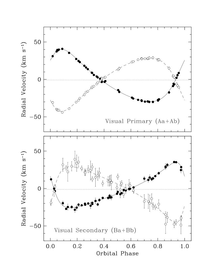
Figure 5.— Radial velocity measurements and computed curves for each of the visual components of HD 110555. The primary star in each spectroscopic binary is represented with filled circles. The center-of-mass velocities are indicated with dotted lines. Error bars for the visual primary components are typically smaller than the size of the points.

References

- Aitken (1908) Aitken, R. G. 1908, Lick Obs. Bull. 4, 166
- Barden (1987) Barden, S. C., ApJ, 317, 333
- Bessell & Brett (1988) Bessell, M. S., & Brett, J. M. 1988, PASP, 100, 1134
- Carpenter (2001) Carpenter, J. M. 2001, AJ, 121, 2851
- Chabrier et al. (2005) Chabrier, G., Baraffe, I., Allard, F., & Hauschildt, P. H. 2005, in Resolved Stellar Populations, ASP Conf. Ser., eds. D. Valls-Gabaud & M. Chavez, in press (astro-ph/0509798)
- Covino et al. (2001) Covino, E., Melo, C., Alcalá, J. M., Torres, G., Fernández, M., Frasca, A., & Paladino, R. 2001, A&A, 375, 130
- Delfosse et al. (2000) Delfosse, X., Forveille, T., Ségransan, D., Beuzit, J.-L., Udry, S., Perrier, C., & Mayor, M. 2000, A&A, 364, 217
- Demarque et al. (2004) Demarque, P., Woo, J.-H., Kim, Y.-C., & Yi, S. K. 2004, ApJS, 155, 667
- ESA (1997) ESA 1997, The Hipparcos and Tycho Catalogues, ESA SP-1200
- Girardi et al. (2000) Girardi, L., Bressan, A., Bertelli, G., & Chiosi, C. 2000, A&AS, 141, 371
- González et al. (2006) González, J. F., Hubrig, S., Nesvacil, N., & North, P. 2006, A&A, 449, 327
- González & Levato (2006) González, J. F., & Levato, H. 2006, A&A, 448, 283
- Griffin et al. (2000) Griffin, R. E. M., David, M., & Verschueren, W. 2000, A&AS, 147, 299
- Hadrava (1995) Hadrava, P. 1995, A&AS, 114, 393
- Harmanec (1998) Harmanec, P. 1998, A&A, 335, 173
- Hartkopf et al. (2001) Hartkopf, W. I. Mason, B. D., & Worley, C. E. 2001, Sixth Catalog of Orbits of Visual Binary Stars, http://www.ad.usno.navy.mil/wds/orb6/orb6.html
- Hill (1993) Hill, G. 1993, in ASP Conf. Ser. 38, New Frontiers in Binary Star Research, eds. K. C. Leung & I.-S. Nha (San Francisco: ASP), 127
- Jha et al. (2000) Jha, S., Torres, G., Stefanik, R. P., Latham, D. W., & Mazeh, T. 2000, MNRAS, 317, 375
- Kurtz & Mink (1998) Kurtz, M. J., & Mink, D. J. 1998, PASP, 110, 934
- Lacy (1977) Lacy, C. H. 1977, ApJ, 218, 444
- Latham (1992) Latham, D. W. 1992, in IAU Coll. 135, Complementary Approaches to Double and Multiple Star Research, ASP Conf. Ser. 32, eds. H. A. McAlister & W. I. Hartkopf (San Francisco: ASP), 110
- Latham et al. (2002) Latham, D. W., Stefanik, R. P., Torres, G., Davis, R. J., Mazeh, T., Carney, B. W., Laird, J. B., & Morse, J. A. 2002, AJ, 124, 1144
- Ling (2004) Ling, J. F. 2004, ApJ, 153, 545
- Mazeh et al. (2001) Mazeh, T., Latham, D. W., Goldberg, E., Torres, G., Stefanik, R. P., Henry, T. J., Zucker, S., Gnat, O., & Ofek, E. O. 2001, MNRAS, 325, 343
- Mermilliod & Mermilliod (1994) Mermilliod, J.-C., & Mermilliod, M. 1994, Catalogue of Mean UBV Data on Stars, (New York: Springer)
- Nordström et al. (1994) Nordström, B., Latham, D. W., Morse, J. A., Milone, A. A. E., Kurucz, R. L., Andersen, J., & Stefanik, R. P. 1994, A&A, 287, 338
- Nordström et al. (2004) Nordström, B., Mayor, M., Andersen, J., Holmberg, J., Pont, F., Jørgensen, B. R., Olsen, E. H., Udry, S., & Mowlavi, N. 2004, A&A, 418, 989
- Pribulla & Rucinski (2006) Pribulla, T., & Rucinski, S. M. 2006, AJ, 131, 2986
- Pribulla et al. (2006) Pribulla, T., Rucinski, S. M., Lu, W., Mochnacki, W. S., Conidis, G., Blake, R. M., DeBond, H., Thomson, J. R., Pych, W., Ogłoza, W., & Siwak, M. 2006, AJ, 132, 769
- Rucinski (2002) Rucinski, S. M. 2002, AJ, 124, 1746
- Simkin (1974) Simkin, S. J. 1974, A&A, 31, 129
- Simon & Sturm (1994) Simon, K. P., & Sturm, E. 1994, A&A, 281, 286
- Skrutskie et al. (2006) Skrutskie, M. F. et al. 2006, AJ, 131, 1163
- Stefanik et al. (1999) Stefanik, R. P., Latham, D. W., & Torres, G. 1999, in Precise Stellar Radial Velocities, IAU Coll. 170, ASP Conf. Ser., 185, eds. J. B. Hearnshaw & C. D. Scarfe (San Francisco: ASP), 354
- Tokovinin et al. (2006) Tokovinin, A., Thomas, S., Sterzik, M., & Udry, S. 2006, A&A, 450, 681
- Tomkin et al. (2007) Tomkin, J., Griffin, R. F., & Alzner, A. 2007, The Observatory, April issue, in press
- Tonry & Davis (1979) Tonry, J. L., & Davis, M. 1979, AJ, 43, 393
- Torres et al. (2006) Torres, G., Lacy, C. H. S., Marschall, L. A., Sheets, H. A., & Mader, J. A. 2006, ApJ, 640, 1018
- Torres et al. (2002) Torres, G., Neuhäuser, R., Guenther, E. W. 2002, AJ, 123, 1701
- Torres et al. (1995) Torres, G., Stefanik, R. P., Latham, D. W., & Mazeh, T. 1995, ApJ, 452, 870
- Willmitch & Fekel (1990) Willmitch, T. R., & Fekel, F. C. 1990, AJ, 99, 373
- Yi et al. (2001) Yi, S. K., Demarque, P., Kim, Y.-C., Lee, Y.-W., Ree, C. H., Lejeune, T., & Barnes, S. 2001, ApJS, 136, 417
- Zucker & Mazeh (1994) Zucker, S., & Mazeh, T. 1994, ApJ, 420, 806
- Zucker et al. (1995) Zucker, S., Torres, G., & Mazeh, T. 1995, ApJ, 452, 863