BLIND MD-MC COMPONENT SEPARATION FOR POLARIZED OBSERVATIONS OF THE CMB WITH THE EM ALGORITHM

We present the PolEMICA $\!{}^{{\bf?}}$ (Polarized Expectation-Maximization Independent Component Analysis) algorithm which is an extension to polarization of the SMICA $\!{}^{{\bf?}}$ temperature component separation method. This algorithm allows us to estimate blindly in harmonic space multiple physical components from multi-detectors polarized sky maps. Assuming a linear noisy mixture of components we are able to reconstruct jointly the electromagnetic spectra of the components for each mode $T$, $E$ and $B$, as well as the temperature and polarization spatial power spectra, $TT$, $EE$, $BB$, $TE$, $TB$ and $EB$ for each of the physical components and for the noise on each of the detectors. This has been tested using full sky simulations of the Planck satellite polarized channels for a 14-months nominal mission assuming a simple linear sky model including CMB, and optionally Galactic synchrotron and dust emissions.

1 Introduction

Mapping the Cosmic Microwave Background (CMB) polarization is one of the major challenges of future missions in observational cosmology. CMB polarization is linear and therefore can be described by the first three Stokes parameters I, Q and U which are generally combined to produce three fields (modes), $T$, $E$ and $B$. The polarization of the CMB photons carries extra physical informations that are not accessible by the study of the temperature anisotropies. Therefore its measurement helps breaking down the degeneracies on cosmological parameters as encounter with temperature anisotropies measurements only. Furthermore, the study of the CMB polarization is also a fundamental tool to estimate the energy scale of inflation.

However, CMB polarization is several orders of magnitude weaker than the temperature signal and therefore, its detection needs an efficient separation between the CMB and the astrophysical foregrounds which are expected to be significantly polarized.

A direct subtraction of these foreground contributions on the CMB data will require an accurate knowledge of their spatial distributions and of their electromagnetic spectra. But these latter are not yet well characterized in polarization.

To try to overcome the above limitations, a great amount of work has been dedicated to design and implement algorithms for component separation which can discriminate between CMB and foregrounds. We present here the PolEMICA (Polarized Expectation-Maximization Independent Component Analysis) algorithm which is an extension of the Spectral Matching Independent Component Analysis (SMICA) $\!{}^{{\bf?}}$ which has been developed to consider both a fully blind analysis for which no prior is assumed and a semi-blind analysis incorporating previous physical knowledge on the astrophysical components. This extension allows to estimate jointly the temperature and polarization parameters from a set of multi-frequencies $I$, $Q$ and $U$ sky maps.

2 Model of the microwave and sub-mm sky

To perform the separation between CMB and the astrophysical foregrounds, the diversity of the electromagnetic spectra and of the spatial spectra of the different components is generally used. Observations from a multi-band instrument, for the Stokes parameters $I$, $Q$ and $U$, can be modeled as a linear combination of multiple physical components leading to what is called a Multi-Detectors Multi-Components (MD-MC) modeling.

Assuming an experiment with $n_{\nu}$ detector-bands at frequencies $\nu_{i}$ and $n_{c}$ physical components in the data, working in the spherical harmonics space, we can model the observed sky for $X=\{T,E,B\}$, for each frequency band and for each $\{\ell,m\}$

$$y^{\nu,X}_{\ell m}=\sum_{c=1}^{n_{c}}A^{\nu,X}_{c}s^{c,X}_{\ell m}+n^{\nu,X}_{\ell m}$$ (1)

where $y^{\nu,X}_{\ell m}$ is a vector of size $(3\cdot n_{\nu}\cdot n_{\ell}\cdot n_{m})$ containing the observed data, $s^{c,X}_{\ell m}$ is a $(3\cdot n_{c}\cdot n_{\ell}\cdot n_{m})$ vector describing each component template and $n^{\nu,X}_{\ell m}$ is a vector of the same size than $y^{\nu,X}_{\ell m}$ accounting for the noise. $A^{\nu,X}_{c}$ is the mixing matrix containing the electromagnetic behaviour of each component and is of size $(3\cdot n_{\nu})\times(3\cdot n_{c})$

The aim of the component separation algorithm presented in here is to extract $A^{\nu,X}_{c}$, $s^{c,X}_{\ell m}$ and $n^{\nu,X}_{\ell m}$ from the $y^{\nu,X}_{\ell m}$ sky observations.

3 A MD-MC component separation method for polarization

To reduce the number of unknown parameters in the model described by equation (1), it is interesting to rewrite this equation in terms of the temperature and polarization auto and cross power spectra and to bin them over $\ell$ ranges.

$$R_{y}(b)=AR_{s}(b)A^{T}+R_{n}(b)$$ (2)

where $R_{y}(b)$ and $R_{n}(b)$ are $(n_{\nu}\cdot 3)\times(n_{\nu}\cdot 3)$ matrices and $R_{s}(b)$ is a $(n_{c}\cdot 3)\times(n_{c}\cdot 3)$ matrix. We assume that the physical components in the data are statistically independent and uncorrelated and that the noise is uncorrelated between channels.

To estimate the above parameters from the data we have extended to the case of polarized data the spectral matching algorithm developed in SMICA $\!{}^{{\bf?}}$ for temperature only. The key issue of this method is to estimate these parameters, or some of them (for a semi-blind analysis), by finding the best match between the model density matrix, $R_{y}(b)$, computed for the set of estimated parameters and the data density matrix $\tilde{R}_{y}(b)$ obtained from the multi-channel data. The likelihood function is a reasonnable measure of this mismatch. We have extended this method to jointly deal with the temperature and polarization power spectra and also to estimate the $TE$, $TB$ and $EB$ cross power spectra $\!{}^{{\bf?}}$.

The maximization of the likelihood function is achieved via the Expectation-Maximization algorithm (EM) $\!{}^{{\bf?}}$. This algorithm will process iteratively from an initial value of the parameters following a sequence of parameter updates called ‘EM steps’. By construction each EM step improves the spectral fit by maximizing the likelihood. For a more detailed review of the spectral matching EM algorithm used here, see $\!{}^{{\bf?}}$.

4 Simulated microwave and sub-mm sky as seen by Planck

Following the MD-MC model discussed above and given an observational setup, we construct, using the HEALPix pixelization scheme $\!{}^{{\bf?}}$ and in CMB temperature units, fake $I$, $Q$ and $U$ maps of the sky at each of the instrumental frequency bands. For these maps we consider three main physical components in the sky emission: CMB, thermal dust and synchrotron. Instrumental noise is modeled as white noise.

The CMB component map is randomly generated from the polarized CMB angular power spectra for a set of given cosmological parameters. In the following we have used $H_{0}=71\ {\rm km}\cdot{\rm s}^{-1}\cdot{\rm Mpc}^{-1}$, $\Omega_{b}=0.044$, $\Omega_{m}=0.27$, $\Omega_{\Lambda}=0.73$ and $\tau=0.17$ that are the values of the cosmological concordance model according to the WMAP 1 year results $\!{}^{{\bf?}}$.

For the diffuse Galactic synchrotron emission we use the template maps in temperature and in polarization provided by $\!{}^{{\bf?}}$. Here we have chosen to use a constant spectral index equal to the mean of the spectral index map, $\alpha=-2.77$, so that the simple linear model of the data holds.

In the case of the thermal dust we dispose of few observational data of the polarized diffuse emission and to date no template for this is available. Thus, we have considered a power-law model, renormalized to mimic at large angular scales the $TE$ cross power spectrum measured by Archeops at 353 GHz $\!{}^{{\bf?}}$. $I,Q$ and $U$ full-sky maps are generated randomly from these power spectra. We extrapolate them to each of the frequency of interest by assuming a grey body with an emissivity of 2.

Noise maps for each channel are generated from white noise realizations normalized to the nominal level of instrumental noise for that channel.

We have performed sets of simulations of the expected Planck satellite data to intensively test the algorithm presented above. We present here results from 300 realizations considering full-sky maps at the LFI and HFI polarized channels, 30, 40 and 70 GHz for LFI and 100, 143, 217 and 353 GHz for HFI for a nominal 14-month survey. We have simulated maps at $n_{\rm side}$ = 512 which permits the reconstruction of the angular power spectra up to $\ell\simeq 1500$. The reconstructed spectra will be averaged over bins of size 20 in $\ell$.

5 Results

We have applied the PolEMICA component separation algorithm to the simulations presented above. From them, we have computed the data density matrix $R_{y}$ and applied the algorithm. We simultaneously estimate the $R_{s}$, $R_{n}$ and $A$ matrices, with no priors, for temperature and polarization. To ensure the reliability of the results we have performed 10000 EM iterations and checked, for each simulation, the convergence of the EM algorithm.

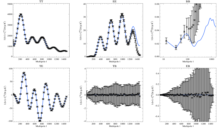
Figure 1: Reconstruction of the CMB power spectra for $C_{\ell}^{TT}$, $C_{\ell}^{EE}$, $C_{\ell}^{BB}$, $C_{\ell}^{TE}$, $C_{\ell}^{TB}$ and $C_{\ell}^{EB}$ at 100 GHz in $\mu{\rm K}_{\rm CMB}^{2}$ performed on Planck full sky maps simulations. Crosses represent the reconstructed spectra, solid lines the input model. Error bars are the dispersion over $\sim$ 300 simulations.

We present in figure 1 the reconstructed CMB power spectra. We can see that for the $TT$, $TE$, $TB$ and $EB$ spectra, we are able to reconstruct the $C_{\ell}$ over the full range of $\ell$ values that are accessible at this pixelization resolution ($\ell_{\rm max}\sim 1500$). The $EE$ spectrum is recovered accurately up to $\ell\simeq 1200$. For smaller angular scales, a bias appears. This bias is a pixelization problem that would occur at a larger $\ell$ if the resolution was higher. The $BB$ spectrum is reconstructed up to $\ell\simeq 70$. For larger $\ell$, the reconstructed spectrum is residual noise arising from the fact that the convergence of the EM algorithm is slow and therefore we have not properly converged. This bias appears in our separation when the signal over noise ratio is below $10^{-2}$ and does not affect the reconstruction of the other parameters. Even if we were able to avoid this effect, the recovered $BB$ spectrum would be compatible with zero for $\ell>70$ thanks to the size of the error bars.

The power spectra from our input synchrotron and dust emissions are recovered with efficiency up to $\ell\simeq 1500$ for $TT$, $EE$, $BB$, $TE$, $TB$ and $EB$ $\!{}^{{\bf?}}$. Power spectra of the noise in temperature and in polarization are also fully reconstructed $\!{}^{{\bf?}}$.

The mixing matrix $A$ elements corresponding to CMB and dust emission are recovered efficiently, for temperature and polarization. For the synchrotron emission, mixing matrix elements corresponding to polarization are well recovered and those corresponding to temperature are biased at intermediate frequency values $\!{}^{{\bf?}}$. This bias is due tu a slight mixing up between synchrotron and CMB in temperature. It does not happen in polarization where the synchrotron dominates the CMB. This bias can be avoided by the adjunction of priors in the separation, like for example assuming an equal electromagnetic spectrum in temperature and polarization for each component $\!{}^{{\bf?}}$

To evaluate the impact of foregrounds in the determination of the CMB temperature and polarization power spectra we have compared the results of the presented analysis to those on simulations that contain only CMB and noise. In the presence of foregrounds, the error bars on the reconstruction of the CMB power spectra are increased by at least a factor of two both in temperature and in polarization $\!{}^{{\bf?}}$. Therefore, although the foreground contribution in the data can be removed, it significantly reduces the precision to which the CMB polarization signal can be extracted from the data.

References

- [1] Aumont J. & Macías-Pérez J.-F., 2007, MNRAS, in press, astro-ph/0603044
- [2] Delabrouille J., Cardoso J.-F. & Patanchon G., 2003, MNRAS, 346, 1089
- [3] Dempster A., Laird N. & Rubin D, 1977, J. of the Roy. Stat. Soc. B, 39, 1
- [4] Giardino G., Banday A. J., Górski K. M., Bennet K., Jonas J. L. & Tauber J., 2002, A&A, 387, 82
- [5] Górski K. M., Hivon E. & Wandelt B. D., 1999, astro-ph/9812350
- [6] Ponthieu N. et al., 2005, A&A, 444, 327
- [7] Spergel D. N. et al., 2003, ApJS, 148, 175