Abstract

In this paper, a relative number density parameter, called the neighborhood function, is introduced so that the crowded nature of the neighborhood of individual sources could be described. With this parameter one can determine the probability of forming a cluster with a given number of galaxy members and a certain number density by chance. A method is proposed to identify large-scale structure on the cosmological co-moving frame. To avoid those effects arising from the distance of objects when applying the method, we compare the real number density concerned with the mean number density measured in the corresponding local area rather than the mean of the whole sample. The scale used to sort out clustering sources is determined by that mean local number density, and thus it is a redshift-dependent scale. In applying this method, the sample adopted is required to have regular borders so that a simulation over the sample area could be performed and the volume confined by the sorting out scale within the sample area could be determined and then the probability referring to number density could be evaluated. The method is applied to a sample drawn from the 2dF survey, analyzed in redshift space. We find from the analysis that the probability of forming the resulting large-scale structures by chance is very small and the phenomenon of clustering is dominant in the local Universe. Within the $3\sigma$ confidence level, a coherent cluster with its scale as large as $357h^{-1}Mpc$ and another with its number of galaxy members as large as 12966 are identified from the sample. There exist some galaxies which are not affected by the gravitation of clusters and hence are suspected to rest on the co-moving frame of the Universe. Voids are likely the volumes within which no very crowded sources are present and they are likely formed in embryo by fluctuation in the very early epoch of the Universe. In addition, we find that large-scale structures are coral-like and they are likely made up of smaller ones; sources with large values of the neighborhood function are mainly distributed within the structure of prominent clusters and it is them who form the frame of the large-scale structure.

Key words: cosmology: observations — galaxies: distances and redshifts — galaxies: statistics — large-scale structure of universe — methods: data analysis

1 Introduction

Distributions of galaxies in the sky were found useful in studying large-scale structures of the Universe (Seldner et al. 1977; Gellar & Huchra 1989; Loveday et al. 1992). Owing to redshift surveys available in different eras, many investigations were made to detect large-scale structures in both the projected map and the three-dimensional space. There were many discoveries of clustering features in 80’s, including voids, galaxy clusters, strings, great attractors, and various great walls (Kirshner et al. 1981; Bahcall & Soneira 1983; Haynes & Giovarelli 1986; Lynden-Bell et al. 1988; Gellar & Huchra 1989). In as early as 1989, the CfA “Great Wall” was found to extend to $170h^{-1}Mpc$ (Gellar & Huchra 1989), while in recent years the Sloan Great Wall was observed to be stretched to $\sim 400h^{-1}Mpc$ in length by Gott III et al. (2005) and by Deng et al. (2006) respectively. The latter is the largest structure of the Universe observed so far. Observations also revealed that large-scale structures could be found deep in the space where redshift is high (Shimasaku et al. 2003; Matsuda et al. 2005; Ouchi et al. 2005). Investigation of large-scale structures of the Universe meets a new chance owing to two recent redshift surveys, the 2-degree Field galaxy redshift survey (2dFGRS) ( Colless et al. 2001) and the Sloan Digital Sky Survey (SDSS) (York et al. 2000) which provide large amount and reliable data.

Large-scale structures of the local Universe are of particular importance since theories of structure formation could be directly checked by redshift surveys. It was predicted that large-scale filamentary or sheet-like mass overdense regions would preferentially be formed in the early Universe and later evolve into dense clusters of galaxies which would be expected in the local Universe, and gravitational amplification of the matter density fluctuations that are generated in the early Universe is assumed to be responsible for the formation of the clustering structure of the present Universe (see Peebles 1982; Blumenthal et al. 1984; Davis et al. 1985, 1992; Governato et al. 1998; Kauffmann et al. 1999; Cen & Ostriker 2000; Benson et al. 2001; Colberg et al. 2005). Filamentary features were found to be real when some redshift surveys were carefully checked (Bhavsar & Ling 1988; Bharadwaj et al. 2000; Bagchi et al. 2002; Ebeling et al. 2004; Pimbblet et al. 2004; Porter & Raychaudhury 2005). The detection of a large concentration of primeval galaxies at redshift $z\sim 3$ (Steidel et al. 1998) and the reported discovery of a large-scale coherent filamentary structure of Ly$\alpha$ emitters in a redshift space at $z=3.1$ favor the prediction that galaxies preferentially formed in large-scale filamentary or sheet-like mass overdensities in the early Universe (Matsuda et al. 2005). In agreement with these, protoclusters which have been presumed not to have virialized due to their short cosmological ages (e.g. Venemans 2005) were identified at as far as $z\sim 4$ (Venemans et al. 2002; Intema et al. 2006).

The great success of cold dark matter (CDM) model in recent years makes it a leading model in current studies of cosmology. The charm of the CDM model is its predictive power on the formation of large-scale structures. However, in this model, large-scale structures up to $>100h^{-1}Mpc$ are rarely formed, which are challenged by recent observations (see Yoshida et al. 2001; Yoshida 2005). It suggests that the CDM model predicts smaller homogeneity scale of the Universe than what the observations have revealed (note that the large-scale structure of the Universe was found to be several hundred $h^{-1}Mpc$). In addition, the model faces difficulty in explaining the observed structure on length scales $<1h^{-1}Mpc$ as well (see a brief review in Cembranos et al. 2005).

Statistical methods are useful in studying large-scale structures of the Universe. As mentioned in Martinez & Saar (2002a), most of the statistical analysis of the galaxy distribution proposed so far are based on second order methods (correlation functions and power spectra) (see also Diggle 1983). Among them, the two-point correlation function (Totsuji & Kihara 1969; Peebles 1974, 1980; Davis & Peebles 1983) and the power spectrum (Fisher et al. 1993; Feldman et al. 1994; Park et al. 1994; Tadros & Efstathiou 1996) are the tools most often used in both observational and theoretical analyses. The latter is the Fourier transform of the former. Since the two quantities are a Fourier transform pair, complete knowledge of one is equivalent to complete knowledge of the other. But this is not true for their estimators when samples employed are finite and noisy (Feldman et al. 1994). The two-point correlation function $\xi(r)$, which was first used to measure the strength of galaxy clustering for redshift surveys by Davis & Peebles (1983), describes the excess probability of finding a galaxy in a volume element at a separation $r$ from another randomly chosen galaxy above that for an un-clustered distribution. There are various estimators of $\xi(r)$ in literature. The main difference is their corrections for the edge effect (Martinez & Saar 2002a). The quantity was found to obey a power law: $\xi(r)=(r/r_{0})^{-\gamma}$ on small scales ($\sim 1-10h^{-1}Mpc$) (for early works, see Totsuji & Kihara 1969; Davis & Geller 1976; Davis & Peebles 1983). In recent investigations, the indexes were found to be $\gamma\sim 1.8$ and $r_{0}\sim 6.1h^{-1}Mpc$ for the SDSS data and $\gamma\sim 1.7$ and $r_{0}\sim 5.1h^{-1}Mpc$ for the 2dFGRS data (Zehavi et al. 2002; Hawkins et al. 2003). As pointed out by Yadav et al. (2005), the power law relation of $\xi(r)$ does not hold on large scales and it breaks down at $r>16h^{-1}Mpc$ for SDSS and at $r>20h^{-1}Mpc$ for 2dFGRS, and thus it would not violate the homogeneous nature of the Universe.

An advantage of the two-point correlation function is its application to galaxy groups to reveal the matter distribution in the Universe, since the occupation of haloes by galaxies is believed to depend on halo mass (see Benson et al. 2000; Berlind et al. 2003). As each dark matter halo is expected to give birth to a single group of galaxies, applying the two-point correlation function to different groups of galaxies one can reveal the clustering nature of these groups and this in turn can tell how dark matter is distributed (see, e.g., Jing & Zhang 1988; Merchan et al. 2000; Zandivarez et al. 2003; Padilla et al. 2004).

In measuring the scale of homogeneity of the Universe, the power spectrum is applicable (see Einasto & Gramann 1993). Martinez et al. (1998) introduced the $K$ function $K(r)$, related to the integral of the two-point correlation function, as a tool. One of their main claims is that the estimators for $K(r)$ are more reliable than the most currently used estimators for $\xi(r)$ and that makes the use of $K(r)$ recommendable (especially in three-dimensional processes and at large scales) despite its somewhat less informative character (see Martinez et al. 1998). In the following one will find that the concept of the $K$ function is also useful in describing the crowded nature of the neighborhood of individual sources and hence able to reveal the density property of a group of sources.

Based on the previous methods, we develop in this paper a statistical approach to sort out clustering sources. Our main concern includes: crowded degrees of sources in their neighborhoods are quantified so that one can tell how different crowded sources form a cluster; redshift dependent densities of samples are taken into account to sort out clusters so that the relevant statistical significance could be determined; via simulation, probabilities for forming clusters by chance are calculated. The method is applied to the 2dFGRS data set. As the results, some fine maps of large-scale structures derived from the sample are available and probabilities of a list of clusters are obtained. The paper is organized as follows. In Section 2, we propose the method, where a statistic called the individual neighborhood function $\kappa_{i}(r)$ is introduced to describe the crowded nature of individual sources. In Section 3, we describe the selection of the sample and study the redshift distribution it obeys. Density distributions of the sample, in terms of $\kappa_{i}(r)$, are presented in Section 4. Clustering probabilities obtained by simulation are studied in Section 5. Coherent clusters are identified and shown in Section 6. In Section 7, we show the structures of some large prominent coherent clusters. In Section 8, the largest structures sorted out from the whole 2dF data set are shown and discussed. In the last section (Section 9), a summary of the paper and a brief discussion are presented.

2 Methods and relevant statistics

2.1 The clustering scale

There are two well-known methods for identifying galaxy groups or clusters. The most popular one is used to create galaxy group catalogues, where a projected separation together with a velocity difference are employed to search for companion sources (Huchra & Geller 1982; Eke et al. 2004; Diaz et al. 2005; Merchan & Zandivarez 2005). A product of this method is the property associated with the virial theorem (e.g., the velocity dispersion of a set of sources), and it is suitable to identify virialized group of galaxies. The other is used to pick out large-scale structures, where a single scale, which is applied to all sources of the sample, is employed to identify a neighborhood source (Einasto et al. 1984; Deng et al. 2006). The main concern of this method is the statistical property (e.g., the length or density) of the identified clusters. In both approaches, the so-called “friends-of-friends” (FoF) algorithm, the claim “any friend of my friend is my friend”, is applied. The latter approach is somewhat suitable for our analysis. However, besides picking out clustering sources, we need to know in what confidence level a group of sources could be regarded as a cluster or with what probability the cluster could be identified by chance. Here, based on the second method, we try to establish a statistical approach to identify large-scale structures, with which the confidence level of selecting a cluster is able to be informed.

In order to develop such a method, we need to address several questions: (1) How do we pick out a cluster? (2) In what confidence level could a cluster with a certain number of galaxies and crowded degree be identified by chance? To find answers to these questions, at least the following requirement should be satisfied: the probability for identifying a group of galaxies as a cluster by chance should be well determined. In doing so, it is essential that all selection effects should be removed or avoided. It is plain that, if the scale used to find coherent clusters is larger than the area concerned, then all sources within that area must be included in a single coherent cluster; if the scale is as small as possible, then all sources within that area must be separated from each other and no coherent clusters could be identified. It seems that, in identifying a group of clustering sources, one needs to take several steps: determine a criterion clustering scale, $r_{ccs}$; sort out clustering sources with $r_{ccs}$ by applying the FoF algorithm; calculate the probability for picking out a cluster by chance. In calculating the probability, the Monte-Carlo simulation will be applicable.

In the case of the two-point correlation function, the correlation length $r_{0}$ is regarded as a characteristic clustering scale. According to the well-known power law relation $\xi(r)=(r/r_{0})^{-\gamma}$, the probability of finding another source, relative to any source concerned, at $r=r_{0}$ is twice the probability produced by random data sets. If the sample is large enough, the twice probability suggests that the density measured at that scale is two times of the mean density. As mentioned above, in the two recent surveys, $r_{0}$ was found to range from $\sim 5.1h^{-1}Mpc$ to $\sim 6.1h^{-1}Mpc$. A criterion associated with the sorting out scale comparable to these scales will be adopted in this paper.

Let $\rho_{0}(z)$ be the mean density of a flux-limited but homogenous data set without the effect of clustering, expected at redshift $z$. Similar to the commonly used selection function (see, e.g., Martinez & Saar 2002b; Coil et al. 2004; Padilla et al. 2004), $\rho_{0}(z)$ as a function of redshift is determined by the real distribution of the observed galaxies at $z$, which depends on the evolutionary effect, and is affected by the flux-limited effect as well as other selection effects such as masks in given fields, fiber collisions in the spectrographs, etc (Martinez & Saar 2002b). As pointed out by Martinez & Saar (2002b), many selection effects are directional, with some being due to the construction of the sample. The absorption by the dust of the Milky Way also gives rise to a selection effect which is also directional. The best way to take this effect into account is to consider the well defined maps of the distribution of galactic dust (Schlegel, Finkbeiner and Davis 1998). When directional selection effects are considered, we should deal with $\rho_{0}(z,\theta,\phi)$ instead of $\rho_{0}(z)$, where $\theta$ and $\phi$ are coordinates of direction. For the sake of simplicity, we consider in this paper only the case of $\rho_{0}(z)$ which corresponds to the commonly used radial selection function. The difference between $\rho_{0}(z)$ and the radial selection function is that, when measuring the former, we divide the count of sources within a redshift interval by the real volume confined by that interval.

The criterion clustering scale adopted in this paper is taken as $r_{ccs}=[2\rho_{0}(z)]^{-1/3}$. The reason for adopting this criterion clustering scale is that the scale so adopted is generally smaller than, but comparable to, the mentioned typical scales $r_{0}$ which range from $\sim 5.1h^{-1}Mpc$ to $\sim 6.1h^{-1}Mpc$ in the two recent surveys. The mean of $r_{ccs}$ in the sample adopted below (sample 2) is $4.2h^{-1}Mpc$. The number of galaxies in the sample with their $r_{ccs}$ being less than $5h^{-1}Mpc$ is 172265, 76% of the total. That means that sources of clusters will generally be sorted out with the scales less than $r_{0}$ (note also that, in Deng et al. 2006, $r\sim 5h^{-1}Mpc$ was adopted to sort out clusters, and in Hoyle et al. 2002, $r=5h^{-1}Mpc$ was used to plot the median density contour). We find that when $r_{ccs}=5h^{-1}Mpc$ is adopted to sort out clusters one will get a much larger number of galaxies for the largest coherent cluster sorted out with the method proposed below. Adopting $r_{ccs}=[2\rho_{0}(z)]^{-1/3}$ will provides us a conservative result. (Note that when adopting $r_{ccs}=[4\pi\rho_{0}(z)/3]^{-1/3}$ one will get a more conservative result since $r_{ccs}$ becomes smaller, but this scale will be much less comparable to $r_{0}$.)

It is known that in the case of the two-point correlation function, $r_{0}$ depends on the clustering property of samples. If adopting $r_{0}$ to identify clusters of a sample, we are going to measure the structure of the sample with a ruler concluded from the structure itself. If the structure changes then the ruler changes. Unlike $r_{0}$, the criterion clustering scale $r_{ccs}$ proposed here depends only on the property of the background sample from which the concerned probability will be derived (see what presented below). This quantity is entirely independent of the properties of the adopted sample and then is a rather objective ruler.

Due to the flux-limited effect, some distant galaxies will be missed. This makes the average distance between distant sources that are observed become larger. If we take a fixed $r_{ccs}$ to identify clusters by applying the FoF algorithm, we might probably include all nearby sources in a single large-scale structure when $r_{ccs}$ is large enough, while it might be possible that for those far away galaxies only very few of them are included to form a cluster since $r_{ccs}$ is not as large as to connect most of them. This is unfair. For some nearby sources, they might in fact be relatively far away from the local structure but they are included as members of the structure since their distances to the structure are shorter than the adopted $r_{ccs}$; for distant sources, since the average distances are large they have less chance to be identified as members of clusters according to this fixed $r_{ccs}$. When we adopt $r_{ccs}=[2\rho_{0}(z)]^{-1/3}$ we deal with a varying $r_{ccs}$ since $\rho_{0}(z)$ is a function of redshift. In this case, we will get a large value of $r_{ccs}$ for large redshifts and obtain a smaller one for small redshifts. As part of out method, a varying $r_{ccs}$ will be adopted to identify clusters (see what proposed below).

2.2 Radial selection function

The result of simulation would be acceptable when the background sample so created has no bias or has only very insignificant bias. It is essential that all selection effects and the evolutionary effect have been removed or avoided. There is a straightforward technique to avoid these effects. Assume that, within a spherical space centered at the observer, there are $N_{0}$ galaxies in total, which form various structures due to dynamics and other known or unknown factors. When no clustering mechanisms are at work, these sources are expected to be homogeneously distributed within the area, and they constitute a global homogenous background sample. In fact, what one can observe at present are galaxies of different cosmological ages. Due to the evolutionary effect, number densities might evolve with redshift, and then the total number, $N$, of galaxies whose photons could reach us at present would be different from $N_{0}$ (e.g., the formation of galaxies and the merging of galaxies might occur somewhere at some time). In this situation, the distribution of the observable background sample would only be homogeneous locally. Let us consider a survey over the whole sky. Due to the flux-limited effect and other selection effects, only $N^{\prime}$ ($N^{\prime}<N$) galaxies could be observed in both real and background samples, which we call the whole observed real sample and the whole observed background sample respectively. (Note that these two samples have the same number of galaxies, but the galaxies are assumed to be distributed randomly in the latter sample.) It is obvious that the mean number densities of the whole observed real sample and the whole observed background sample would be the same in different redshifts, from which we can deduced a mean number density law with respective to redshift. Now we perform a survey over a limited area of the sky. According to the isotropic nature of the Universe, it is expected that the mean number densities of this smaller observed real sample and the corresponding observed background sample are the same as well in different redshifts. Keeping this in mind, a background sample created by the simulation following this mean number density law would have no bias. Statistical significance derived from this sample would be safely acceptable. Note that selection effects would differ from survey to survey due to different techniques and instruments. The proposed simulation method is simple due to the fact that it does not refer to the details of selection effects (in fact, all selection effects have been taken into account).

Besides the selection effects, there exists the boundary effect for most samples. It is desired that problems arising from this effect could be overcome. The most effective way of solving this problem is to consider the real volume involved. In the case of estimating $\xi(r)$, the count of sources of the adopted sample lying inside the shell $[r-\Delta r/2,r+\Delta r/2]$ relative to a point is divided by the volume of the intersection of that shell with the whole sample volume (Rivolo 1986; Martinez et al. 1998, 2001). This technique will be adopted in our analysis.

Based on these arguments, we propose: a) for a survey concerned, search for the mean number density law $\rho_{0}(z)$ with the whole data set; b) draw from the survey a subsample for which the borders are regularly cut so that within these borders a sub background sample could be easier created according to $\rho_{0}(z)$; c) for a given redshift, determine the sorting out coherent clustering scale by $r_{ccs}(z)=[2\rho_{0}(z)]^{-1/3}$; d) apply the FoF algorithm with $r_{ccs}(z)$ to identify clustering sources; e) calculate the probability of creating a cluster with a given number of galaxies and density by chance. In doing so, the real volume confined by $r_{ccs}(z)$ and the whole area of the subsample will be considered when calculating the relevant density (see what presented below) so that the boundary effect would be avoided (see Rivolo 1986; Martinez et al. 1998, 2001).

What effects does varying $r_{ccs}(z)$ have on the analysis when the above method is applied? As discussed above, the missing of objects due to the flux-limited effect will make $\rho_{0}(z)$ becoming smaller and thus make $r_{ccs}(z)$ becoming larger. Two possibilities will occur in this situation: some intrinsic clustering sources are missed and some intrinsic unclustered objects are included in a cluster identified with the method. This will make the sorting out clusters less convincing at large distances where galaxies are rare. The probability for mis-identifying sources is currently unavailable since the real distribution of galaxies is unaware.

2.3 Definition and estimation of the neighborhood function

The concept of clusters indicates the phenomenon of a number of sources gathering within a relatively small volume. It is directly associated with high density regions. The two-point correlation function is not a direct measurement of number density of the neighborhood of individual sources and cannot describe the crowded nature (the degree of density) of their neighborhoods. The same number found within the same volume of shells relative to two sources does not guarantee that the same amount of neighborhood galaxies would be detected within the area enclosed by the shells (this could be observed in the galaxy distribution plot of many surveys). To measure the crowded nature of individual sources as well as the density of a cluster, we need a proper quantity which could be applicable to a discrete source sample.

There is a quantity suitable to describe the crowded nature of the neighborhood of discrete sources. It is the conditional density in spheres $\Gamma^{*}(r)$ which is an ensemble of realizations of a given point process (see Coleman et al. 1988; Joyce et al. 1999, 2005; Vasilyev et al. 2006). Motivated by this quantity and the $K$ function mentioned above in the introduction section, we introduce in the following a new statistic to describe the crowded nature of the neighborhood of individual sources, where the mean density as a function of redshift and the boundary effect are taken into account.

Consider a real sample with number of galaxies $N$ and a background sample of the same number of galaxies, confined within the same volume. The latter sample is created by simulation under the assumption that galaxies are randomly distributed according to $\rho_{0}(z)$ over the space concerned. Assign $\eta(\overrightarrow{r})$ as a density function defined by

$$\eta(\overrightarrow{r})\equiv\frac{\rho(\overrightarrow{r})}{\rho_{0}(z)}-1$$ (1)

in the co-moving coordinates of the Universe, where $\rho(\overrightarrow{r})$ is the number density of the sample concerned at position $\overrightarrow{r}$, and $\rho_{0}(z)$ is the mean density of the background sample expected at the redshift corresponding to $\overrightarrow{r}$. Concerning the crowded nature of the neighborhood (the neighborhood density) of a source, let us introduce an individual neighborhood function $\kappa_{i}(r)$ for object $i$ to describe the number density of the sample relative to the object within scale $r$, which is defined by

$$\kappa_{i}(r)\equiv\frac{\int_{V_{i}(r)}\rho(\overrightarrow{r})dV}{\rho_{0}(z_{i})V_{i}(r)}-1,$$ (2)

where $z_{i}$ is the redshift of object $i$, and $V_{i}(r)$ is the volume of the intersection of the sphere with radius $r$, centered at object $i$, with the whole volume of the adopted sample (here, $r$ does not represent $|\overrightarrow{r}|$). The mean of $\kappa_{i}(r)$ of a sample (called the neighborhood function of the sample),

$$\kappa(r)\equiv\frac{1}{N}\sum_{i}^{N}\kappa_{i}(r),$$ (3)

is one of its statistical properties (a spatial distribution property), which reflects the mean relative number density of the sample measured within the mentioned scale (note that, in the case of adopting $r=r_{ccs}$, $r$ will differ from source to source). For a subset of the sample (namely, a group of sources of the sample), we also use the mean of $\kappa_{i}(r)$ to describe its spatial distribution property (its density nature), and this quantity is also denoted by $\kappa(r)$. The only difference is that, in equation (3), $N$ will be replaced by $N^{\prime}$, where $N^{\prime}$ is the number of galaxies of the subset. It is obvious that the larger the $\kappa(r)$, the more crowded the sample or the group. In terms of $\eta(\overrightarrow{r})$, the two quantities could be expressed by

$$\kappa_{i}(r)=\frac{\int_{V_{i}(r)}\eta(\overrightarrow{r}_{i})dV}{V_{i}(r)}$$ (4)

and

$$\kappa(r)=\frac{1}{N}\sum_{i}^{N}\frac{\int_{V_{i}(r)}\eta(\overrightarrow{r}_{i})dV}{V_{i}(r)}.$$ (5)

(Note that, when different weights for the particles are adopted and taken into account, one might deal with other definitions of $\kappa_{i}(r)$ and $\kappa(r)$. In that situation, one might wish to modify definition (1) so that the forms of other equations would maintain.)

In the case of the two-point correlation function, $\xi(r)>0$ suggests that, for any given source, the probability of finding another source in distance $r$ is larger than the probability produced by the random data set and the former is $1+\xi(r)$ times of the latter. In the case of the individual neighborhood function, the probability of finding a source within the scale of $r$ relative to position $\overrightarrow{r_{i}}$ is proportional to the integral of the number density $\rho(\overrightarrow{r})$ over the volume confined by $|\overrightarrow{r}-\overrightarrow{r_{i}}|<r$ for the adopted sample, and it is $1+\kappa_{i}(r)$ times of that of the background sample which is created randomly according to $\rho(z)$, where $\kappa_{i}(r)>0$ suggests the larger probability of the sample than that of the background sample. In the case of the neighborhood function, the probability of finding a source within the scale of $r$ is $1+\kappa(r)$ times of that of the background sample.

In practice, $\kappa_{i}(r)$ and $\kappa(r)$ can be computed by

$$\kappa_{i}(r)=\frac{1}{\rho_{0}(z_{i})\Delta V_{i}(r)}\sum_{j}^{|\overrightarrow{r}_{j}-\overrightarrow{r}_{i}|<r}\int n_{j}dV-1$$ (6)

and

$$\kappa(r)=\frac{1}{N}\sum_{i}^{N}[\frac{1}{\rho_{0}(z_{i})\Delta V_{i}(r)}\sum_{j}^{|\overrightarrow{r}_{j}-\overrightarrow{r}_{i}|<r}\int n_{j}dV]-1,$$ (7)

where $n_{j}$ is the $\delta$-function giving the position of particle $j$; $\Delta V_{i}(r)$ is the portion of the whole sample volume satisfying $|\overrightarrow{r}-\overrightarrow{r}_{i}|<r$ for any position $\overrightarrow{r}$; the integral takes over $\Delta V_{i}(r)$; the sum over $j$ includes only particles in the position within $|\overrightarrow{r}_{j}-\overrightarrow{r}_{i}|<r$ in the sample, which yields the number of sources found within $\Delta V_{i}(r)$. For a volume limited sample, $\Delta V_{i}(r)$ would differ from source to source due to different positions of the objects relative to the borders of the sample volume, even $r$ is the same.

One can check that, when ignoring the variation of $\rho_{0}(z)$ with respect to redshift, then quantity $1+\kappa(r)$ would be similar to the Ripley $K$ function which is an integral of $1+\xi(r)$ over the spherical ball with radius $r$ (Ripley 1981; Martinez et al. 1998). There is not a direct relation between $\kappa(r)$ estimator and commonly used $\xi(r)$ estimators since we calculate $\kappa(r)$ in a slightly different manner [e.g., no random samples are required to compute $\kappa(r)$]. However, when the difference between $1+\kappa(r)$ and the Ripley $K$ function is ignored, then the differential of $1+\kappa(r)$ would come to $1+\xi(r)$. The main difference between the $K$ function, or the two-point correlation function, and the neighborhood function is that, with $\kappa_{i}(r)$ we can tell how crowded is the neighborhood of a source and can even show how different crowded sources are distributed in the space and how this distribution is related to the structures observed (see what presented below).

Quantity $\kappa(r)$ could also be closely related to the conditional density in spheres $\Gamma^{*}(r)$ (Vasilyev et al. 2006). In applying equation (7), when one takes $\rho_{0}(z_{i})=1$ and makes the sum over the whole sample, $1+\kappa(r)$ would become $\Gamma^{*}(r)$, as long as the volume of the sample concerned is large enough so that for any point in the sample the sphere of radius $r$ centered at the point is well inside the volume.

In the following analysis, cosmological distances as well as co-moving volumes will be expressed in terms of the co-moving coordinates and in calculating the latter the standard cosmological model, $(\Omega_{M},\Omega_{\Lambda})=(0.3,0.7)$, will be adopted through out this paper, leaving the Hubble constant parameter $h$ ($H_{0}=100hkms^{-1}Mpc^{-1}$) serving as a unit. The analysis will be performed in redshift space. That is, when calculating the co-moving coordinates of galaxies of samples drawn from redshift surveys, the peculiar velocity of individual sources will be ignored and the measured redshift will be taken as the real distant indicator of the object.

3 Sample selections and redshift distributions

The data studied are taken from “The 2dF galaxy redshift survey (2dFGRS): final data release” (Colless et al. 2003). Two main regions of the survey data located in distinct areas of the sky are visible. To calculate $\kappa_{i}(r)$ as well as $\kappa(r)$, we must know the volume $\Delta V_{i}$ for each source and for any given $r$. This would be realizable if the area concerned is well defined where its borders are sharp. The computation would be easier performed if the edges of a region are regularly cut. The following criterions are adopted to select a sample from the survey data set: $150.0^{\circ}<R.A.(J2000)<220.0^{\circ}$, $-4.8^{\circ}<Dec.(J2000)<1.0^{\circ}$, $0.0<z<0.3$, $quality\geq 3$, where $quality$ is the redshift quality parameter for best spectrum ($quality=1-5$; reliable redshifts have $quality\geq 3$). We thus get a sample of 59497 sources (called sample 1). Table 1 presents the description of this sample as well other samples mentioned below, where column 1 is the name of samples, columns 2, 3 and 4 denote the number, area and region of the samples respectively, column 5 shows the $\rho_{0}(z)$ that is used to calculate $\kappa$ for the samples and to create the corresponding background samples by simulation (see what mentioned below), and column 6 denotes the type of data (observation or simulation, with the former being that of a real sample and the latter being that of a background sample). The sky region of sample 1 is illustrated in figure 1, where one of the two distinct areas, which encloses this sample, is also presented.

We notice that there are shortcomings of the 2dF sample. As shown in Cannon et al. (2006), there are fibre collisions within 2dF, where many objects around the edge of a 2 degree field are missed (see figure 3 in Cannon et al. 2006). This would give rise to a directional incompleteness of a survey. However, the provided data are from such a set of 2 degree fields where most regions of the sky inside the survey boundary are covered by several overlapping fields and the potential incompleteness has been significantly reduced (see figure 5 in Colless et al. 2003). In addition, we cut away the edge of the concerned region and this reduces the directional effects of fibre collisions as well. We thus presume in this paper that the effect of this is minor (i.e. ignorable).

Another shortcoming is the existence of “missed galaxies” (see Pimbblet et al. 2001; Cross et al. 2004). As shown in Cross et al. (2004), the incompleteness of the sample could reach about 14 per cent, which varies slightly with magnitude (see figure 11 of the paper). This shortcoming is a selection effect. As a function of redshift, it is absorbed into $\rho_{0}(z)$ (see what adopted below). The main influence of this effect on our results is that when we identify a large-scale structure with the current 2dF data we might obtain a larger one when all missed galaxies are discovered.

The third shortcoming is due to the fact that the $b_{J}=19.45$ magnitude limit is not constant across the entire area of the survey (see Colless et al. 2001; Norberg et al. 2002). This might affect the results of the analysis. We will discuss this effect in the last section of this paper.

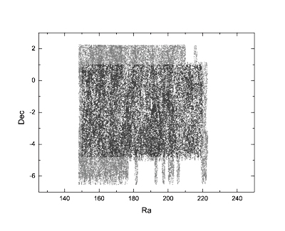
Figure 1: Sky region of sample 1 (dark grey color), in coordinates of $R.A.(J2000)$ and $Dec.(J2000)$. The parent area where sample 1 is taken from is also presented (both dark and light grey colors).

Since the volume of the area concerned is well defined, we are now able to estimate the mean density of the background sample, $\rho_{0}(z)$, from the observational data. As pointed out by Padilla et al. (2004), there are several approaches to do so. The most straightforward way is to use the luminosity function of galaxies to obtain an estimate of $\rho_{0}(z)$. This is not adopted in this paper since any bias from the real luminosity function would cause systematic errors (see Padilla et al. 2004 and the references therein). In the following, let us consider three other approaches. The first way is to estimate $\rho_{0}(z)$ directly from the observational data. In this approach we assume that the redshift distribution of the whole 2dF survey data set could serve as a parent population of the background sample. Of course, to match the data of sample 1, the data set serving as the parent population, which covers the whole area of the 2dF survey, should meet these criterions: $0.0<z<0.3$, $quality\geq 3$. A set of 226302 sources (called sample 2) is obtained, which is almost four times of the number of galaxies of sample 1. As illustrated below, there are two massive superclusters in 2dF and these superclusters are comparable to the survey volume (see also Erdogdu et al. 2004; Lahva and Suto 2004; Porter & Raychaudhury 2005; Einasto et al. 2006a). This suggests that 2dF might not be a fair sample of the Universe. The reason for assuming the whole 2dF survey data set being a fair sample of the Universe is that it is indeed very large (based on it, many statistical analyses have been made) and it is the largest available sample of this kind (detected by the same means of the 2dF survey). Under this assumption, we simply measure $\rho_{0}(z)$ from sample 2 and then apply it to our simulation analysis. The advantage of this approach is that any possible evolutionary and selection effects, known or unknown, will be accounted for. There are two disadvantages of the method. One is due to the measurement uncertainty which will cause an unreal distribution within the uncertainty scale. This will be eased by assigning a random value smaller than the uncertainty to the background data when randomly drawing them from sample 2 (the following application shows that this technique is indeed at work; see figure 3). The other is due to the fact that the 2dF survey does not covers the whole sky. If there exist strong clusters which are comparable to the regions concerned (yes, as pointed out above, there are some), the redshift distribution of the presumed parent population will be affected: bumps will be seen in the very dense place and troughs will exist in the very sparse space. In this situation, some redshift distribution feature due to clustering (Padilla et al. 2004) will be mistaken as the background property and then clusters corresponding to this feature might be missed (at least in the redshift space this clustering property will be ignored). Thus, the number of galaxies of some very large clusters would become smaller. To get a safer number of galaxies, one might prefer this approach.

The second way of estimating $\rho_{0}(z)$ is to fit parametric forms to the observational data (see Padilla et al. 2004), which uses sample 2 as well. In this approach, we do not directly apply $\rho_{0}(z)$ that is measured from sample 2 to create background samples. Instead, we fit it with an empirical curve. As long as the probability obtained from the fit is small enough, the fitting curve will serve as $\rho_{0}(z)$ and then will be applied to our simulation analysis. The mean density curve so obtained is nothing but a deep smoothing of that directly measured from sample 2. We have a risk in employing this approach. In the process of smoothing, while bumps and troughs caused by clustering will be smoothed, features arising from selection effects will be smoothed as well. In the following analysis, results arising from the first and the second approaches will be presented and compared.

For the sake of comparison, the third way of estimating $\rho_{0}(z)$ is also adopted. In this approach, the galaxies observed are assumed to be homogenously distributed over the whole area of sample 1. Thus we simply take $\rho_{0}(z)=const$ to create background samples. Although the redshift distribution of this kind of background sample is not real, but the analysis might reveal some aspects of clustering which are unfamiliar before (see what presented below).

Let us derive $\rho_{0}(z)$ from sample 2. The count observed within any sky region of the 2dF survey is assumed to be proportional to the corresponding sky area according to the isotropic property of the Universe. Let $z_{i}$ be the redshift of source $i$ in sample 2. We calculate the count within the redshift interval $0.99z_{i}$ — $1.01z_{i}$ from sample 2 as well as calculate the volume $V(\Delta z_{i})$ confined by this redhift interval in the area of sample 1. According to the isotropic assumption, the volume confined by this redshift interval in the whole area of sample 2 should be $226302/59497$ times of $V(\Delta z_{i})$. Thus the count divided by $(226302/59497)V(\Delta z_{i})$ will be taken as the estimated value of $\rho_{0}(z)$ for this source, which is denoted by $\rho_{0}(z_{i})$. In doing so, when the redshift interval is less than the measurement uncertainty of the survey, the latter will be taken as the width of the redshift interval.

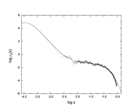
Figure 2: Relation between the mean number density of sample 2 (pluses) and redshift, where the solid line is the fitting curve of the data.

The estimated values of $\rho_{0}(z_{i})$ of sample 2 are shown in figure 2. The data could be well fitted by the following polynomial function: $\log\rho_{0}(z)=-(11.2931\pm 0.0049)-(20.585\pm 0.013)\log z-(15.587\pm 0.011)(\log z)^{2}-(4.9779\pm 0.0039)(\log z)^{3}-(0.52885\pm 0.00045)(\log z)^{4}$ ($P<0.0001$ ), where $\rho_{0}(z)$ is in units of $(Mpc/h)^{-3}$.

We create a background sample (sample 3) randomly from sample 2 with the first approach. The second background sample (sample 4) is produced with the second approach by simulation according to the empirical mean number density function, the polynomial function. The third background sample (sample 5) is yielded by simulation under the assumption that the galaxies are homogenously distributed, where the mean number density is obtained by dividing 59497 with the whole volume of sample 1, which gives $\rho_{0}=0.00247(Mpc/h)^{-3}$. The numbers of galaxies of all these background samples are the same as that of sample 1, $N=59497$.

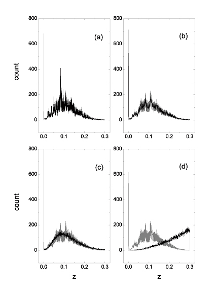
Figure 3: Redshift distributions of samples 1 (black lines in panel a), 2 (grey lines in all panels), 3 (black lines in panel b), 4 (black lines in panel c), and 5 (black lines in panel d). Here, the number of galaxies of sample 2 is normalized to that of sample 1.

Redshift distributions of samples 1-5 are shown in figure 3. Panel (a) of the figure shows that there indeed exist some bumps and troughs in both samples 1 and 2. Compared with other panels, we suspect that this phenomenon is unlikely to be caused by random. Instead, it might probably be due to intrinsic distributions such as large-scale structures (see what discussed above in this section and see Fig. 22 presented below) or selection effects. In addition, we find some significant features in sample 1, which are much less prominent in sample 2. This must be due to the local property of redshift distribution and might probably be a consequence of the existence of local clustering (see Figs. 17, 20 and 21 presented below). Panel (b) plainly demonstrates that samples created with the first approach well follow the redhsift distribution of sample 2. In addition, it reveals that the chaos of the observational samples is largely caused by the measurement uncertainty (since adding an additional random value smaller than the uncertainty significantly reduces the fluctuation observed, as panel b shows). From panel (c) we observe that, when ignoring the fluctuation, which might be caused by local clustering, the polynomial function could indeed well represent the real distribution of the observational samples. Panel (d) illustrates that, as expected, the sources observed are not homogenously distributed at all (the flux-limited effect and the evolutionary effect would be the main factors accounting for the non-homogenous distribution observed in the survey data).

Although spatial distributions of sources of background samples 3 and 4 differ significantly from that of the real homogenous one, sample 5, a distribution in agreement with the former is still regarded as a homogenous one in the following analysis. This is because that background samples 3 and 4 suffer from the flux-limited effect and the evolutionary effect as well as other known or unknown selection effects, and it is these effects that lead to the apparent in-homogenous distribution. When all galaxies of the same cosmological age are available, the spatial distribution of background sample sources, which are randomly created, must be homogenous due to the principle of cosmology. Therefore, in the analysis below, those in agreement with the spatial distribution of sources of the adopted background sample, or in agreement with that of the parent population of background samples, will be regarded as an intrinsic homogenous one, and those obviously deviating from that distribution will be considered as an in-homogenous one.

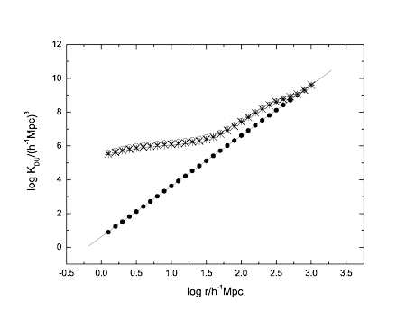
Figure 4: Plot of standard $K$ functions estimated from samples 1 (open circles), 3 (pluses), 4 (crosses), and 5 (filled circles). The solid line is the best linear fit to the $K$ function of sample 5, which obeys $logK_{DU}=(0.623\pm 0.003)+(2.996\pm 0.002)logr$. The correlation dimension could be easily figured out from the plot, where $D_{2}=3$ is obtained for sample 5 and $D_{2}<3$ could be derived from the other three samples within the maximum scale of the samples, $r_{max}=837h^{-1}Mpc$.

Shown in figure 2, one could observe a deviation, of the polynomial provided for $\rho_{0}(z)$, from the mean number density function directly measured from sample 2. In addition, a deviation of the redshift distribution of the polynomial function from that of the $\rho_{0}(z)$ of sample 2 is seen in figure 3 (see panels b and c). This suggests that the polynomial provided for $\rho_{0}(z)$ and the $\rho_{0}(z)$ measured from sample 2 are not the same. However, as one will see below, this difference does not cause big problems in the clustering analysis performed in this paper. Since sample 2 suffers from the clustering effect, as mentioned above and revealed below, it might be possible that samples 3 and 4, which come from sample 2, would be inhomogeneous not only due to the flux limit but also due to clustering. Thus, if the deviation observed in figure 2 leads to an observable difference in the homogeneity properties of the two corresponding background samples needs to be checked. Let us check this by examining their $K$ functions, from which the corresponding correlation dimension $D_{2}$ could be derived (see Martinez et al. 1998). The $K$ function adopted to investigate this issue is that provided in equation (8) of Martinez et al. (1998), the standard estimator introduced by Doguwa and Upton (1989) to account for the boundary effect. As is generally known, regardless of the possible slight bias, this estimator, $K_{DU}$, has good properties. Displayed in figure 4 one could find the $K$ functions estimated from samples 3 and 4, where, for a comparison, that from samples 1 and 5 are also presented. As expected, the $K$ function estimated from sample 5 well follows the homogeneity curve, the curve for which $D_{2}=3$. The three other samples are seen not to be homogeneous at all (for all of them, $D_{2}<3$ holds within the maximum scale of the samples). It is interesting that the $K$ functions estimated from samples 1, 3 and 4 follow almost the same trend (in this case, they will have almost the same $D_{2}$). While that from sample 1 is slightly larger than that of samples 3 and 4, the difference between the latter two cannot be detected. This suggests that, the $K$ function, and hence the derived $D_{2}$, suffers mainly from the redshift distribution which is influenced by the flux limit, the possible evolutionary effect, and the spatial distribution of large-scale structure members (see Fig. 3). The role that the locally clustering (sources in sample 1 are strongly clustered while those in samples 3 and 4 are not; see the spatial clustering plots presented below) plays in producing the correlation dimension $D_{2}$ seems very insignificant.

4 Density distributions

Here, we use estimator (6) to calculate the individual neighborhood function of sources in the scale of $r_{ccs}$ (i.e., we take $r=r_{ccs}$) which is determined by $r_{ccs}=[2\rho_{0}(z)]^{-1/3}$. We apply the $\rho_{0}(z_{i})$ directly measured from sample 2 to calculate $\kappa_{i}(r_{ccs})$ for each source of samples 1 and 3. In addition, we determine $\rho_{0}(z)$ by the polynomial function obtained above and then calculate $\kappa_{i}(r_{ccs})$ for each source of samples 1 and 4 with this $\rho_{0}(z)$. Also, we adopt $\rho_{0}=0.00247(Mpc/h)^{-3}$, the mean number density of sample 1, to calculate $\kappa_{i}(r_{ccs})$ for each source of samples 1 and 5. In this way, we calculate $\kappa_{i}(r_{ccs})$ for sample 1 with three kinds of $\rho_{0}(z)$ (and hence with three kinds of $r_{ccs}$) estimated with three approaches.

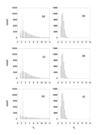
Figure 5: Distributions of the individual neighborhood function for samples 1 (black lines in panels a, c, and e), 3 (black lines in panel b; light grey lines in panel a), 4 (black lines in panel d; light grey lines in panel c), and 5 (black lines in panel f; light grey lines in panel e). The individual neighborhood functions presented in panels (a) and (b) are calculated with the values of $\rho_{0}(z)$ directly estimated from sample 2 (the first approach); those in panels (c) and (d) are calculated with the values of $\rho_{0}(z)$ determined by the empirical polynomial function (the second approach); and that in panels (e) and (f) are calculated with the constant mean density $\rho_{0}=0.00247(Mpc/h)^{-3}$ (the third approach).

Distributions of the individual neighborhood function $\kappa_{i}(r_{ccs})$ of sample 1, calculated with three kinds of $\rho_{0}(z_{i})$ are presented in panels (a), (c) and (e) of figure 5 respectively. Meanwhile, distributions of $\kappa_{i}(r_{ccs})$ of samples 3, 4 and 5 are displayed in panels (b), (d) and (f) of the figure, respectively. One might observe from panels (b), (d) and (f) that the distributions of $\kappa_{i}(r_{ccs})$ are almost the same for background samples created with different approaches, although the adopted $\rho_{0}(z)$, and hence $r_{ccs}$, differs in different cases. This is not surprising since $\kappa_{i}(r_{ccs})$ reflects only a relative density and background samples are randomly created by simulation, which would be locally homogeneous. In fact, the number density of a background sample is created in accordance with a provided mean density $\rho_{0}(z)$, and quantity $1+\kappa_{i}(r_{ccs})$ is that number density divided by the mean density. In the case of a real sample, the situation is much different. In panel (e), when calculating $\kappa_{i}(r_{ccs})$, the number density of sample 1 is divided by a constant mean density, $\rho_{0}=0.00247(Mpc/h)^{-3}$, but the real number density of sample 1 differs significantly for sources with different values of redshift. Thus, one observes a much different $\kappa_{i}(r_{ccs})$ distribution of sample 1 in panel (e) from those in panels (a) and (c). The values of $\kappa_{i}(r_{ccs})$ could be found as large as several ten thousands (the figure covering the whole range of value of the quantity is omitted). In fact, $\kappa_{i}$ in panel (e) reflects absolute number densities rather than locally relative ones. Due to several selection factors mentioned above, there is an enormous difference of observed density. In contrast, distributions of $\kappa_{i}(r_{ccs})$ presented in panels (a) and (c) are almost the same. This suggests that the difference of $\rho_{0}(z)$ shown in figure 2 does not significantly influence the distribution of $\kappa_{i}(r_{ccs})$ for the adopted real sample, sample 1. (See also the discussion below in the case of spatial distributions.)

One might observe that, as histogram plots, distributions in figure 3 look like “continuums” since the total number involved is very large. However, with the same number, those in figure 5 do not look like “continuums” but look like “histograms”. We have checked that this difference is not due to the adopted bins. The distribution plots shown in figure 5 look like “histograms” because in some separated ranges of $\kappa_{i}(r_{ccs})$ the counts are relatively small, while in the nearby $\kappa_{i}(r_{ccs})$ ranges the corresponding counts are large (thus, the former counts look like to be zero). This phenomenon is due to the small scale we adopt (i.e., $r_{ccs}$). Since the scale is relatively small (see the definition of $r_{ccs}$ presented above), one could only find small numbers of sources within the corresponding volume. Thus, the difference of number would lead to obvious difference of the individual neighborhood function. For example, the volumes confined by $r_{ccs}$ would differ slightly for two closely located sources. If the number of neighborhood galaxies relative to one source is 3 and that relative to the other is 4, then this difference would cause a 30 percent of change (in this situation it would be hard to get 3 percent of change for this two sources). At least within a small region enclosing these two sources, the change of a smaller percent would not be observed from the difference of numbers other than 3.

For the background samples, the individual neighborhood function is mainly distributed within the range of $\kappa_{i}(r_{ccs})<3$ (see panels b, d and f), while for sample 1, a large amount of sources have their $\kappa_{i}(r_{ccs})$ larger than $3$ (see panels a, c and e).

Motivated by figure 1 of Governato et al. (1998), let us symbolize a region within which the initial matter forms a galaxy in later times with a presumed galaxy (the matter is referred to as the presumed galaxy matter) and assign the central position of the region as the position of that presumed galaxy. These presumed galaxies are expected to be randomly scattered in space. In terms of statistics, they are considered as un-cluttering sources. In our analysis, $\kappa_{i}(r_{ccs})$ distributions of unclustered galaxies are those displayed in panels (b), (d) and (f) of figure 5. The $\kappa_{i}(r_{ccs})$ distribution of sample 1 is obviously different from them (see panels a, c and e). Revealed in the figure, a large amount of sources in sample 1 possess very large values of $\kappa_{i}(r_{ccs})$ (say, $\kappa_{i}>3$) which the majority of unclustered galaxies do not have, suggesting that there is clustering in this sample.

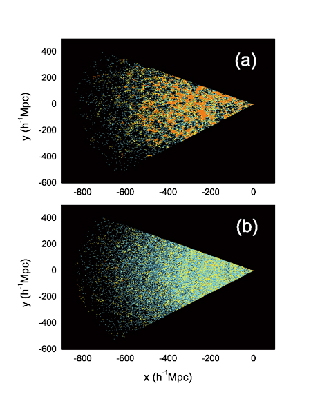
Figure 6: Spatial (two dimensional) distributions of different crowded sources in samples 1 (panel a) and 3 (panel b), measured in the criterion clustering scale $r_{ccs}$. The values of $\rho_{0}(z)$ directly estimated from sample 2 are adopted to determine $r_{ccs}$ and to calculate $\kappa_{i}$. The cyan color stands for un-crowded sources (sources with relatively low number densities in their neighborhoods; $-1\leq\kappa_{i}<1$) (a lot of cyan color objects are not observed in this figure due to the overlap of other color objects), the yellow color represents crowded sources (sources with relatively large number densities in their neighborhoods; $1\leq\kappa_{i}<3$), and the orange color symbolizes very crowded sources (sources with relatively very large number densities in their neighborhoods; $3\leq\kappa_{i}$). The co-moving coordinates are determined by $x=Dsin(\pi/2-Dec)cos(Ra)$, $y=Dsin(\pi/2-Dec)sin(Ra)$, $z=Dcos(\pi/2-Dec)$ (here $z$ is a coordinate, as generally adopted; when it represents a redshift in the text below, we will present a note), where $D$ is the distance of the object to the observer, in units of $h^{-1}Mpc$.

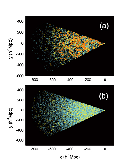
Figure 7: Spatial (two dimensional) distributions of different crowded sources in samples 1 (panel a) and 4 (panel b), measured in the criterion clustering scale $r_{ccs}$. The values of $\rho_{0}(z)$ figured out from the empirical polynomial function are adopted to determine $r_{ccs}$ and to calculate $\kappa_{i}$. The symbols are the same as they are in figure 6. For the definition of the coordinates, see figure 6.

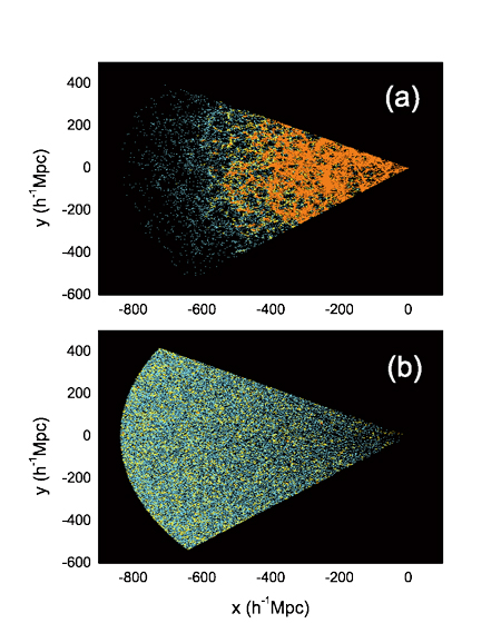
Figure 8: Spatial (two dimensional) distributions of different crowded sources in samples 1 (panel a) and 5 (panel b), measured in the criterion clustering scale $r_{ccs}$. The mean density $\rho_{0}=0.00247(Mpc/h)^{-3}$ evaluated from sample 1, which is a constant with respect to redshft, is adopted to determine $r_{ccs}$ and to calculate $\kappa_{i}$. The symbols are the same as they are in figure 6. For the definition of the coordinates, see figure 6.

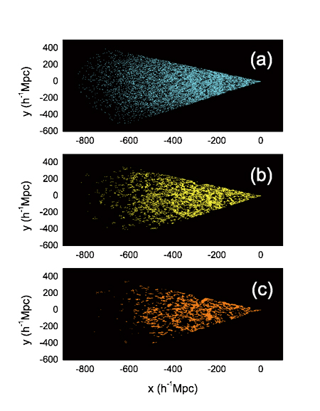
Figure 9: Spatial (two dimensional) distributions of un-crowded (panel a), crowded (panel b) and very crowded (panel c) sources in sample 1, measured in the criterion clustering scale $r_{ccs}$. This plot is a copy of panel (a) in figure 6, where different crowded sources are presented in different panels.

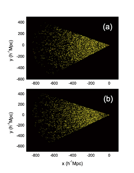
Figure 10: Spatial (two dimensional) distributions of crowded and very crowded sources in samples 3 (panel a) and 4 (panel b), measured in the criterion clustering scale $r_{ccs}$. Panel (a) in this figure is a copy of panel (b) in figure 6, while panel (b) in this figure is a copy of panel (b) in figure 7, where the un-crowded sources are omitted.

According to figure 5 (compare the right- and left-hand-side panels), we define those galaxies with $-1\leq\kappa_{i}<1$, $1\leq\kappa_{i}<3$ and $3\leq\kappa_{i}$ as un-crowded, crowded and very crowded sources, respectively. In other words, sources with $-1\leq\kappa_{i}<1$, $1\leq\kappa_{i}<3$ and $3\leq\kappa_{i}$ are identified as those locally located in regions with relatively small, large and very large number densities of galaxies, respectively. They have different relative number density environments. The spatial distributions of different crowded sources for samples 1, 3, 4, and 5 are displayed in figures 6-8. As expected, one can find from panel (a) of figures 6 and 7 that very crowded galaxies seem to form the core of large-scale structures, where surrounding the core are those less crowded sources (for identifying large-scale structures, see the analysis below). Although in the case of adopting the mean number density, the number of very crowded sources identified from sample 1 (panel a in figure 8) is very large (45753 sources, 77% of the total number of the sample) due to the smaller value of the density, $\rho_{0}=0.00247(Mpc/h)^{-3}$, the region these sources occupy is smaller than that in other cases. (In panel a of figures 6 and 7, the numbers of very crowded galaxies are 27312 and 27476, respectively.) Also as expected, all the un-crowded, crowded and very crowded sources in the background samples are seen to be homogenously (relative to the expected observed density $\rho_{0}(z)$) distributed over the whole sample volume (see panel b in the three figures) (a similar issue will be investigated below; see figure 16). We find that un-crowded sources in sample 1 show a homogenous distribution over the whole sample volume, which could be clearly seen in figure 9 (panel a) (see also figures 15 and 16 presented below) (note that many distant sources are missed due to the flux limited effect). It suggests that some isolated resided matter regions remain to be isolated from the very beginning to late times (during this period, they form galaxies themselves). Crowded and very crowded galaxies in sample 1 are much less homogenously distributed (see panels b and c in figure 9). This might be due to the continuous action of gravity that pulls these galaxies together, as expected in many models. Governato et al. (1998) have already pointed out that large concentrations are common in a universe dominated by cold dark matter and they are the progenitors of the rich galaxy clusters seen today. It is interesting that filamentary features are observed in the state of random distribution, formed particularly by crowded sources (see panel b in figures 6 and 7). This is plainly shown in figure 10. In addition, seeds of knots seem to be presented early in the random state as well (see figure 10). According to the view of Governato et al. (1998), we suspect that it might be these features that grow to the obvious clustering structure observed in later times, where many un-crowded presumed galaxies have joined. It seems that, in this process, very dense regions move towards each other, and some of them form large-scale structures themselves in later times. This is just the case expected in the concentration process of dark matter (see figure 1 of Governato et al. 1998). Revealed by recent observations, filamentary large-scale structures do exist at redshift as large as $z\sim 6$ (Ouchi et al. 2005).

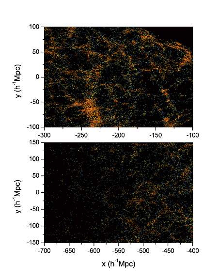
Figure 11: Spatial distributions of different crowded sources of sample 1 in two local regions of the whole volume of the sample (see figure 6 panel a), where the upper panel presents the plot in a region closer to us while the lower panel shows the map in a distant region. The density symbols are the same as they are in figure 6. For the definition of the coordinates, see figure 6.

Observed in the two dimensional map of very crowded sources in sample 1 are some voids (see figure 9 panel c). These voids are also detected in the spatial distribution of crowded sources in the sample, but they are less obvious (see figure 9 panel b). On the contrary, we find no obvious voids in the spatial distribution of un-crowded galaxies in the same sample. Meanwhile, some embryonic voids are seen in the two dimensional plot of crowded sources in sample 3 (see figure 10 panel a). It suggests that voids are likely the volumes within which no or very few very crowded sources are present and they are likely formed in embryo by fluctuation in the very early epoch of the Universe. It might be the continuous gravitation in later times that pulls more crowded galaxies closer and at the same time leaves behind adult voids. Shown in figure 11 are the finer resolution maps showing the details of the spatial distributions of different crowded sources in sample 1 in two local regions of the volume concerned (see figure 6 panel a). Indeed, from the figure we find that, if voids are identified according to the spatial distribution of very crowded sources, then they are seen to be filled mainly with un-crowded sources (for a more detail, see figure 21 presented below).

The spatial density distributions of sample 1 calculated in the first and second approaches are almost the same (see panel a in figures 6 and 7). Meanwhile, one might observe that the distributions of $\kappa_{i}(r_{ccs})$ for sample 1 calculated with the two approaches are not distinguishable (see panels a and c in figure 5). This suggests that the adopted values of $\rho_{0}(z)$ estimated directly from sample 2 and evaluated by the empirical polynomial function do not provide a significant difference in the analysis of density distribution. As discussed above, in examining homogeneity properties of background samples, where the values of the correlation dimension $D_{2}$ are checked, the same conclusion is obtained. In the following, we discuss only the case of adopting the $\rho_{0}(z)$ directly estimated from sample 2 (the first approach), where radial selection effects (known and unknown) are accounted for.

5 Clustering probabilities

As long as the mean density $\rho_{0}(z)$ is available, we are now able to apply the FoF algorithm to identify clustering sources with the scale of $r_{ccs}(z)$. To calculate the probability of creating a cluster with a given number of galaxies (in terms of statistics, the total number of members of a sample is always referred to as the size of the sample) and with a certain number density by chance, we perform a number of simulations and for each time of simulation we sort out coherent clusters and calculate their neighborhood functions. Let the number of simulations when clusters with numbers of galaxies larger than $n^{\prime}$ and neighborhood functions larger than $\kappa^{\prime}$ are observed be $\Delta N$, and the total number of trial be $N$. Then the probability of creating a cluster with its number of galaxies larger than $n^{\prime}$ and its neighborhood function larger than $\kappa^{\prime}$ by chance is estimated by dividing $\Delta N$ with $N$: $P\{n>n^{\prime},\kappa>\kappa^{\prime}\}=\Delta N/N$.

The details of our simulation analysis are summed below (some of them could be found in the previous sections). a) We randomly select 59497 redshifts from sample 2. These form a simulation sample which has the same number of sample 1. In doing so, 226302 redshifts which correspond to 226302 sources contained in sample 2 have the same chance for being selected. (In this way, the redshift distribution of the simulation sample would be the same as that of sample 2. See figure 3 panel b.) b) For each redshift that is selected, we assume that the digital number that is un-measurable is uniformly distributed within the range of that digital number and then we modify the redshift according to this assumption. For instance, when selecting a redshift of 0.2981 from sample 2, we assume that this observed redshift arises from a real redshift ranging within $0.29805<z<0.29815$, and then we modify the original redshift 0.2981 by adding a random value $x$ to it, where $x$ is assumed to be uniformly distributed within the range of $-0.00005<x<0.00005$. We then get a new redshift set for the simulation sample. (As shown in figure 3 panel b, the distribution of redshifts of this kind of sample is much less scattered than that of sample 2.) c) Corresponding to each redshift of the simulation sample, we randomly select a sky position confined in the area of sample 1 and assign the redshift and the position to a source. In this way, we get 59497 sources for the simulation sample. In doing so, the Universe is assumed to be isotropic and then the same area in the sky within the sample region (the area of sample 1; see figure 1) has the same probability for being selected. d) We calculate $r_{ccs}$ for each source in the simulation sample by applying the relation $r_{ccs}=[2\rho_{0}(z)]^{-1/3}$, where the adopted $\rho_{0}(z_{i})$ is that directly measured from sample 2. e) For this simulation sample, we apply the FoF algorithm with the $r_{ccs}$ obtained above to sort out clusters. For each pair of sources we always have two values of $r_{ccs}$. The two sources are considered to be within a same cluster when the distance between them is smaller than the smaller value of the two $r_{ccs}$. f) For each cluster, we calculate their $\kappa(r_{ccs})$, using estimator (7), where the sum is taken over the whole number of sources of the cluster concerned. g) We perform a number of simulation and then, according to these simulations, estimate the probability for forming a cluster with a certain number of galaxies and certain value of $\kappa(r_{ccs})$ by chance.

Besides the reason proposed above, there is one more reason for choosing $-0.00005<x<0.00005$ as the range of $x$ to be added to the provided redshift of sample 2. That is, the treatment itself makes the redshift distribution of the selected sample much less scattered than that of sample 2 (see figure 3 panel b). In this way, the chaos caused by the un-measurable digital number of the redshifts is eased. In doing so, we do not use the real redshift errors since they are not taken into account when we deal with sample 1. In fact, as shown by panel (b) of Figs. 6 and 7, spatial distributions of samples 3 and 4 are not distinguishable, although their redshift distributions are quite different in finer redshift intervals (see figure 3). One can check that replacing $-0.00005<x<0.00005$ with the real redshift errors in the simulation analysis would not provide an observable difference.

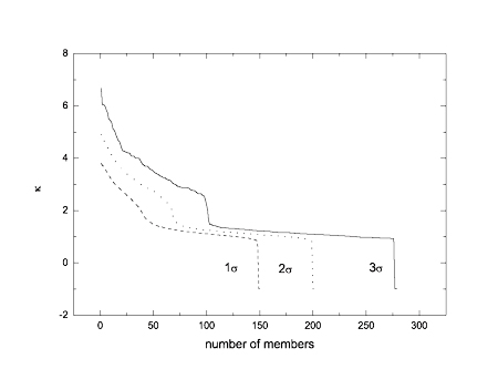
Figure 12: Map of probability contours of coherent clusters formed by chance, where the dashed, dotted, and solid lines represent the probabilities of $1\sigma$, $2\sigma$, and $3\sigma$, respectively.

Displayed in figure 12 are the probability contours of coherent clusters formed by chance (here, $N=5000$). It shows that clusters with larger numbers of galaxies and larger number densities (larger $\kappa$) are harder to be formed. The probability of forming coherent clusters with their numbers of galaxies larger than 350 is less than that of $3\sigma$, $P(3\sigma)$.

Our analysis shows that, if a cluster with its number of galaxies $n$ larger than 10 and its $\kappa$ larger than 5.41 could be formed by chance, the probability must be less than that of $3\sigma$, $P(3\sigma)$. Under the same requirement of probability, other typical pairs of $(n,\kappa)$ are $(100,2.24)$, $(200,1.10)$ and $(300,-0.99)$. It shows that, for a cluster with very large number of galaxies (say, $n>300$), the requirement of $\kappa$ is very weak. It could be a negative one. This suggests that clusters with very large number of galaxies are very hard to be formed by chance. Even when their mean densities are smaller than the average (i.e., $\kappa<0$), they are still very hard to be formed. Thus, when a cluster containing the number of galaxies larger than 300 is identified in an area as large as that of sample 1, it is unlikely that this cluster is formed by chance.

6 Identifying and classifying coherent clusters

Applying our method to samples 1 and 3, we get entirely different sets of coherent clusters. In sample 1, we detect 67 coherent clusters under the condition that if any of them is formed by chance then the probability will be less than that of $3\sigma$. Listed in Table 2 are the parameters of these coherent clusters. Here, the scale of a coherent cluster is defined as the largest value of the distance measured for each pair of the sources of the cluster. The smallest neighborhood function is $\kappa=1.79$. For other 66 clusters, $\kappa>2$. The largest number of galaxies is 12966 and the largest scale is $357h^{-1}Mpc$, which belong to different coherent clusters. For all these clusters, $\kappa>1$, suggesting that the number density, measured for each source within the scale of $r_{ccs}(z)$, for any of these clusters is larger than twice of the mean of the background sample. For sample 3, the largest number of galaxies of the detected coherent clusters is 135 and the neighborhood function of this cluster is $\kappa=1.22$. The number of galaxies is larger than 134, but its neighborhood function is slightly less than that coupling with 134, $\kappa=1.29$ (see figure 12). Thus, the probability of forming this cluster by chance is larger than that of $3\sigma$. The scattering distribution in the plane of $(number,\kappa)$ of the coherent clusters detected from sample 3 is shown in figure 13. Demonstrated in the figure, there are no coherent clusters detected within the $3\sigma$ probability region for sample 3. Displayed in figure 13 is also the scattering distribution of the coherent clusters detected from sample 1. One finds from this figure that almost all of coherent clusters detected from sample 3 are distributed beyond the $1\sigma$ probability region in the plane of $(number,\kappa)$. While a sufficient number (67) of coherent clusters sorted out from sample 1 are situated within the $3\sigma$ probability region, there are some others detected from the sample existing within the region confined by the $1\sigma$ and $3\sigma$ probability contours.

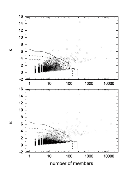
Figure 13: Plot of $\kappa$ vs. number of galaxy members of coherent clusters identified in samples 1 (crosses) and 3 (pluses), where the probability contours in figure 12 are also presented.

We define coherent clusters with probabilities being less than that of $3\sigma$ as prominent clusters, and define those with probabilities being less than that of $1\sigma$ but larger than that of $3\sigma$ as less prominent clusters, and call those with probabilities being larger than that of $1\sigma$ as weak clusters.

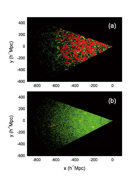
Figure 14: Spatial (two dimensional) distributions of clustering sources of samples 1 (panel a) and 3 (panel b). The blue color stands for un-clustering sources, the green color represents sources of weak clusters, the yellow color denotes sources of less prominent clusters, and the red color symbolizes galaxies of prominent clusters. For the definition of the coordinates, see figure 6.

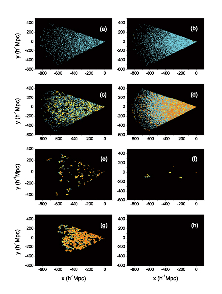
Figure 15: Spatial (two dimensional) distributions of un-clustering sources (panels a and b; the blue color in figure 14), weak clusters (panels c and d; the green color in figure 14), less prominent clusters (panels e and f; the yellow color in figure 14), and prominent clusters (panels g and h; the red color in figure 14) for samples 1 (panels a, c, e, and g) and 3 (panels b, d, f, and h). The color symbols represent the same as they do in figure 6. For the definition of the coordinates, see figure 6.

Spatial (two dimensional) distributions of the three kinds of cluster as well as the unclustered sources for the two samples are shown in figures 14 and 15. We find that the unclustered sources of both the observed and background samples are homogenously distributed over the whole space concerned (see also figure 16 panels a and b). They act like what the low relative density ($-1\leq\kappa_{i}<1$) galaxies do (see figure 9 panel a), and indeed, almost all of them are low relative density galaxies (see figure 15 panels a and b). As suggested in panels (a) and (b) of figure 15, the number of unclustered sources detected from sample 3 is larger than that of sample 1. This is expectable since many original unclustered regions (the presumed galaxies) might be pulled towards a nearby relatively dense region (a presumed cluster) in later times due to the continuous action of gravity. Figure 15 shows that the majority of mid and high relative density sources (those of $1\leq\kappa_{i}<3$ or $\kappa_{i}\geq 3$) are members of clusters (weak, less prominent, or prominent clusters). Compared with the corresponding panels in figure 16 we find that sources of weak clusters in the background sample are homogenously distributed over the whole volume of the sample as well, and the spatial distribution of sources of this kind in the observational sample is a quasi-homogenous one (see panels c and d in figures 15 and 16). In addition, we find that the number of weak clusters in the background sample is also larger than that in the observational sample. This indicates that many unclustered galaxies and weak clusters become members of large-scale structures formed in later times. As expected, shown in panels (e), (f), and (g) of figure 15, we find that the core of prominent and less prominent clusters is filled mainly by sources with high number density neighborhoods ($3\leq\kappa_{i}$), and surrounding them, galaxies with lower number density environments are observed.

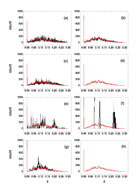
Figure 16: Redshift distributions of un-clustering sources (black lines in panels a and b), weak cluster sources (black lines in panels c and d), less prominent cluster sources (black lines in panels e and f), and prominent cluster sources (black lines in panels g and h) for samples 1 (panels a, c, e, and g) and 3 (panels b, d, f, and h). Red lines denote the redshift distribution of all sources in sample 3 (black lines in figure 3 panel b). Numbers of galaxies of all data sets are normalized to that of sample 1.

The numbers of unclustered, weak clustering, less prominent clustering, and prominent clustering sources of sample 3 are 9033, 50126, 338 and 0, respectively. They occupy 15.2%, 84.2%, 0.568% and 0% of the total number of the sample. The numbers of the corresponding sources in sample 1 are 3557, 12700, 3017 and 40223 respectively, and they are 5.98%, 21.3%, 5.07% and 67.6% of the total. This reveals that, in terms of statistics (i.e., under the $3\sigma$ confidence level), the majority of galaxies observed in the 2dF survey are members of prominent clusters (in about 67.6%). This indicates that the phenomenon of clustering is prominent in the present Universe. Only a few galaxies (about 5.98%) are identified to be sources lonely staying in the space. Comparing the corresponding numbers in the two samples we find that about 2/3 original unclustered sources and 3/4 original weak clustering sources would change their identification in late times. It indicates that original weak clustering sources have more chance to become members of less prominent and prominent clusters in later times and indeed they provide about 87% of members of the latter (note that only about 13% members of the latter come from the original unclustered sources). This is not surprising since the seeds of clusters formed in later times are expected to be among those originally resided in regions with higher number densities (see panel d of figure 15). Displayed in figure 16 are redshift distributions of unclustered, weak clustering, less prominent clustering, and prominent clustering sources of samples 1 and 3. As expected, redshift distributions of different kinds of source in the background sample are well in agreement with the distribution of the sample itself since no dynamics are at work in the stage of random. (Note that the redshift distribution of less prominent clustering sources is not in agreement with that of the whole sample, which is due to the very small number of this kind of source, 0.568%, of the sample). While the redshift distribution of the unclustered sources of the observational sample is consistent with that of the background sample (see panel a of figure 16), there is a slight deviation from that of the weak clustering sources of sample 1 to that of the background sample, and an obvious deviation from that of the prominent clustering sources of sample 1 to that of the latter sample is observed. In addition we find that, for the observational sample, there is a change from weak clusters to prominent clusters: the number of sources in between (sources of less prominent clusters) is relatively small.

According to this analysis, we suspect that there might exist three kinds of galaxy or galaxy group in terms of clustering. One is the class made up of isolated galaxies which would be homogenously distributed over the Universe and would never be included in any clusters. Positions of these galaxies would stick to the framework of the Universe. Another class includes trivial coherent clusters which would act like the isolated galaxies but their number densities would evolve with time. The other class contains prominent coherent clusters whose densities and numbers of galaxies would glow all the time from the very early epoch to present. After the clustering process of all galaxies in the Universe ceases, the redshift distribution of the sources of these clusters would be that of the homogenous spatial distribution, when measured in the volume much larger than that associated with their typical scales. Measured within the volume comparable to that associated with their typical scales, it would not be surprising if the redhsift distribution shows a character of in-homogenous spatial distribution. Before the clustering process stoping, some potential members of these clusters look like trivial coherent clusters in densities (described by $\kappa$) and numbers of galaxies, and this would make the redshift distribution of apparent trivial coherent clusters (weak clusters defined in this paper; see panel c in figure 15) deviates from that of the homogenously spatial distribution (see panel c in figure 16). In this scheme, less prominent clusters defined in this paper should be the potential members of the third class, and they would change their identification in late times. According to this interpretation, once a prominent cluster is formed it will maintain its identification in late times. This explains why there is a turn over change from the number of weak clustering sources to that of prominent clusters observed above.

Revealed in figure 13, there are two approaches for a weak cluster becoming a member of prominent clusters: increasing either its density (described by $\kappa$) or its number of galaxy members. In the first approach, they can accomplish the identification changing themselves when their members become closer, while in the second approach, the change would happen in the situation that they are coherently connected with other clusters. For an isolated cluster, when its relative density stops glowing, the process of identification changing will be ended. This is why we expect a homogenous spatial distribution of members of the second class.

The reasons that we propose the above scheme to interpret the clustering process of galaxies are: a) we find it natural to explain what we observe in the above clustering plots; b) it looks simple; c) it can provide unambiguous predictions in the clustering process which can be checked later; d) we find no simpler schemes accounting for our results.

In the above analysis, we first classify four kinds of source according to their clustering properties available from observation: unclustered sources (which do not appear in figure 13), weak clustering sources (which are beneath the $1\sigma$ contour in figure 13), less prominent clustering sources (which are within the area confined by the $1\sigma$ and $3\sigma$ contours in figure 13), and prominent clustering sources (which are above the $3\sigma$ contour in figure 13). Later we propose a scheme with three kinds of galaxy or galaxy group (isolated galaxies, trivial coherent clusters, and prominent coherent clusters) to explain what we observed in the statistical analysis. The four kinds of source might change their identifications during the clustering process. But when the clustering process ceases, each of them belongs to one of the three kinds of galaxy or galaxy group.

7 Structure of large prominent coherent clusters

Here we show the structure of the two largest prominent coherent clusters identified in sample 1. According to Table 2, the coherent cluster with the largest number of galaxies is cluster 1 which contains 12966 galaxies and extends to $281h^{-1}Mpc$; the one with the second largest number of galaxies is cluster 2 which contains less galaxy members (7788) but has the largest scale, $357h^{-1}Mpc$. The scale of cluster 1 is the distance between the two sources TGN141Z157 and TGN353Z218, and that of cluster 2 is the distance between TGN163Z153 and TGN276Z102. Displayed in figure 17 are the two-dimensional positions (relative to that of other galaxies of sample 1) of the two coherent clusters. Shown in figures 18 and 19 are their plane and solid structures, viewed from various angles in the latter case.

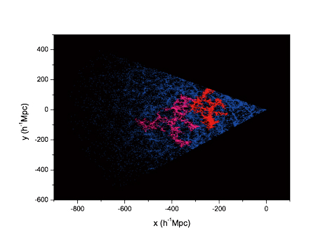
Figure 17: Two-dimensional positions of the two largest coherent clusters identified from sample 1, where the red and pink colors represent clusters 1 and 2, respectively. Sources other than the two clusters are presented in the blue color. For the definition of the coordinates, see figure 6.

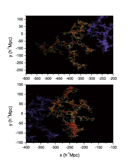
Figure 18: Two-dimensional map of the structures of the two largest coherent clusters detected from sample 1. Presented in the lower panel is that of cluster 1, where the violet color represents the sources of cluster 2. Shown in the upper panel is that of cluster 2, where the violet color represents the sources of cluster 1. The royal and blue colors stand for un-crowded sources (the royal color for $-1\leq\kappa_{i}<0$ and the blue color for $0\leq\kappa_{i}<1$), the cyan and yellow colors represent crowded sources (the cyan color for $1\leq\kappa_{i}<2$ and the yellow color for $2\leq\kappa_{i}<3$), and the orange and wine colors symbolize very crowded sources (the orange color for $3\leq\kappa_{i}<6$ and the wine color for $6\leq\kappa_{i}$). (Note that, here we use six colors instead of only three to code different crowded sources in order to show their spatial distributions in a more detail. The colors used are somewhat different from those adopted in figure 6.) For the definition of the coordinates, see figure 6.

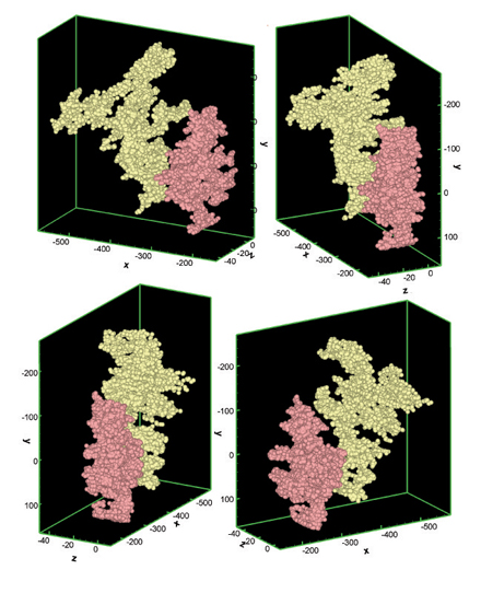
Figure 19: Three dimensional map of the structures of the two largest coherent clusters, where the yellow color represents cluster 1 and the magenta color denotes cluster 2. Here, a relatively lower resolution map is presented so that the solid structure is noticeable. For the definition of the coordinates, see figure 6.

As shown in figure 17, the two clusters are quite close. The scales of the two coherent clusters are comparable with the whole volume of sample 1 (the upper limit of redshift in sample 1 is $z=0.3$ which corresponds to $r\sim 837h^{-1}Mpc$; see also figure 17). This might interpret why there is a bias of the redshift distribution of prominent coherent clusters of sample 1 to the redhsift distribution of the whole background sample (see figure 16 panel g, especially at $z\sim 0.082$ which corresponds to $r\sim 241h^{-1}Mpc$). Revealed by figure 18, very crowded sources form the core as well as the frame of the corresponding structures. The two clusters possess coral type structures in a fine map where the details of the structure are visible. It seems that larger coherent clusters are made up of smaller ones and in forming the former the latter are likely connected by their antennae. This is in agreement with what was discovered recently by Einasto et al. (2006b): superclusters are asymmetrical and have multi-branching filamentary structure.

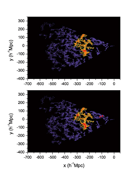
Figure 20: Two-dimensional positions of clusters (the red color) detected by Erdogdu et al. (2004) (the upper panel) and Eke et al. (2004) (the lower panel). For the sake of comparison, cluster 1 identified in this paper from sample 1 is presented with the same coded colors adopted in figure 6. Sources of other prominent clusters identified from sample 1 are also presented which are coded with the violet color. The two filled circles in the upper panel denotes the the redshift range where SCNGP06 (Erdogdu et al. 2004) is detected and located. The filled circles in the lower panel stand for central positions of the nine large galaxy number groups detected from NGP, presented in Table A2 of Eke et al. (2004). For the definition of the coordinates, see figure 6.

In the same volume studied above, Erdogdu et al. (2004) detected a large cluster, SCNGP06. We find that SCNGP06 is just inside the structure of cluster 1, which is shown in figure 20. Eke et al. (2004) also identified large galaxy number groups in the same volume. Among their 9 largest groups identified within the volume, 7 are inside the structure of cluster 1 (see figure 20). Revealed in the figure, centers of SCNGP06 and the 7 large galaxy number groups of Eke et al. (2004) are located at the knots of the structure.

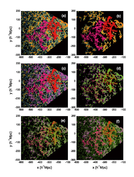
Figure 21: Two-dimensional structures of clusters 1 (red) and 2 (pink) and the spatial distribution of different crowded galaxies of sample 1 within the same area. In panel (a), colors other than the red and pink denote all sources other than those of the two clusters within the area, and these sources are coded with the same colors as they are coded in figure 6. Panel (b) is a copy of panel (a), where sources other than those of prominent clusters are taken off. Panel (c) is also a copy of panel (a), where sources of prominent clusters other than clusters 1 and 2 are symbolized by the magenta color. In panels (d), (e), and (f), the red, pink, and magenta colors represent sources of cluster 1, cluster 2, and all other prominent clusters, respectively. Green colors in panels (d), (e), and (f) stand for all very crowded, crowded, and un-crowded sources in sample 1 within the area, respectively. For the definition of the coordinates, see figure 6.

As suggested above (see figure 9 panels b and c), voids are likely the volumes within which no crowded sources are present. In the structures of the two largest coherent clusters, voids are easily identified (see figure 18). Are they really the space where no crowded sources are found? Figure 21 shows the structures of the two clusters together with that of other prominent clusters and the spatial distribution of different crowded galaxies of sample 1 within a smaller area enclosing the structures. We find from panel (a) of the figure that, for the majority of voids detected from the structures of the two clusters, there indeed no or very few high density galaxies are present. This can be clearly seen in panels (d) and (e). Within the apparent void of $(x,y)\sim(-300,-50)h^{-1}Mpc$ in panel (a), there are some very crowded sources. We suspect that this might not be a real void, but instead, it might come from the projected effect. In other words, the inner structures observed within the apparent void might not be close to the two clusters in the three-dimensional space, but they look like to be close to them in the projected two-dimensional space. Indeed, as revealed in panels (b) and (c), inside the apparent void, some structures of prominent clusters are present. Shown in panel (d), there are indeed few very crowded sources outside the structures of prominent clusters, and it is these galaxies that form the core and build the frame, of the structures. Crowded sources tend to be gathered around the structures, as seen in panel (e). Just as pointed out above, un-crowded sources are seen to be homogenously distributed over the structure area, and they are indeed detected within the voids as well as within the frame of the structures (see panel f). In a recent investigation of voids, Patiri et al. (2006) showed that faint galaxies populating the voids are clustered in small groups and filaments. This is observed in panel (f). In addition, we find that the apparent filaments of un-crowded galaxies do not stretch along the frame of the structure of the prominent clusters, as what the very crowded and crowded sources do in panels (d) and (e). Recalled that filamentary features could appear in the state of random distribution (see the discussion in Section 4), we thus suspect that the apparent filaments of low density galaxies might mainly be caused by fluctuation.

8 The largest structure detected in a larger data set of the 2dF survey

One might observe that, in the method adopted above, while the calculation of the relevant probability and the investigation of number density distribution depend on the exact volume of the adopted sample, the sorting out method (i.e., the FoF algorithm) is independent of the volume. This enables us to identify the largest scale structure of a sample of the same survey, for which, the borders are not well defined and the volume is not available. Although the probability of forming such structure by chance is unable to be evaluated, at least the following questions might be able to answer. How large is the scale of the largest structure identified from the whole 2dF survey by the FoF algorithm? Could some unconnected structures identified in a smaller volume be coherently connected in a larger volume, which is strongly expected? Is the coral type structure detected in the space of sample 1 merely a local nature? (Or, could it be found in other areas of the survey?).

Here, we apply the sorting out method proposed above to the whole 2dFGRS data set. To match the basic criterions of sample 1, we simply adopt sample 2 for our analysis. The $\rho_{0}(z)$ used to determine the $r_{ccs}$ is that directly measured from sample 2 (i.e., $\rho 1$ in Table 1).

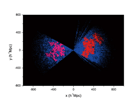
Figure 22: Two-dimensional positions of the two largest coherent clusters detected from sample 2, where the red and pink colors represent the largest and the second largest coherent clusters, respectively. Sources other than the two clusters are presented in the blue color. For the definition of the coordinates, see figure 6.

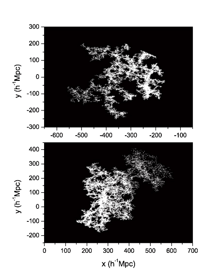
Figure 23: Two-dimensional map of the structures of the two largest coherent clusters detected from sample 2. Presented in the lower panel is that of the largest coherent cluster, and shown in the upper panel is that of the second largest coherent cluster. For the definition of the coordinates, see figure 6.

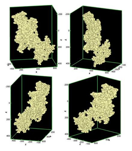
Figure 24: Three dimensional map of the structure of the largest coherent cluster identified from sample 2. Here, a relatively lower resolution map is presented so that the solid structure is noticeable. For the definition of the coordinates, see figure 6.

The largest number of galaxies of the coherent clusters identified in sample 2 is 41813, and the scale of this cluster is $659h^{-1}Mpc$ which is the largest one detected with the adopted method. The second largest cluster contains 32188 galaxies and its scale is $474h^{-1}Mpc$. The two-dimensional positions (relative to that of other galaxies of sample 2) of the two coherent clusters are illustrated in figure 22 which shows that the structures of the two groups of galaxies are situated in two distinct areas of the sky. Comparing it with figure 17 we find that the two largest coherent clusters identified from sample 1, clusters 1 and 2, now become a single one, the second largest cluster identified from sample 2 (the one shown in the left-hand side of figure 22). Besides those of clusters 1 and 2, some other sources are also included in the second largest cluster. This is expectable, since the area of sample 1 is well inside that of sample 2 in that direction of the sky (see figure 1), and some bridge sources outside the area of sample 1 might exist and then would connect clusters 1 and 2 together as well as connect other sources or clusters to them. The right-hand side of figure 22 shows that large-scale structures could extend to the space as far as the adopted samples could reach (the largest redshift detected in the right-hand side structure, the largest coherent cluster detected from sample 2, is $z=0.2646$). (For the left-hand side structure, the largest redshift detected is $z=0.1969$.) This indicates that the large-scale structure is not a patent right of nearby galaxies. Instead, it could be formed in a quite early time, although space sampling is sparse at that epoch (see figure 8 panel a). In fact, it was found in recent observations that large structures are common at redshifts as large as $z\sim 3$ (Steidel et al. 1998). Large-scale structures which are made up of protoclusters could be formed even at the epoch as early as $z\sim 6$ (Ouchi et al. 2005).

The structure of the largest cluster detected from sample 2, that in the right-hand side of figure 22, is displayed in figures 23-24, where more details are visible (shown in figure 23 is also the two dimensional structure of the second largest cluster). Figure 23, which is a fine map, shows that the topology of the structure is coral-like as well.

Although the probability for forming the two largest coherent clusters by chance is not available due to the ill-defined borders of sample 2, we tend to believe that the two clusters are not formed by chance. According to figure 12, large numbers of galaxies of coherent clusters are scarcely formed by chance, even their mean relative densities are small. In sample 3, the largest number of galaxies is much less than 300 (see figure 13), but the largest one detected from sample 1 is 12966 which is 43 times of 300. The largest and the second largest numbers of galaxies of the coherent clusters identified from sample 2 are 139 and 107 times of 300, respectively. It is unlikely that the enhancement of the volume from sample 1 to sample 2, where the number of galaxies of the latter is about 4 times of the former, would shift the $3\sigma$ probability contour in figure 13 to the number of galaxies as large as that of the second largest cluster, 32188 (a detailed analysis on this issue will be performed later).

9 Discussion and conclusions

Our analysis is performed in redshift space, where the peculiar velocity of individual sources is ignored. As is known, in measuring the distance of an object, a big problem is the joining of its dynamical velocity to the redshift observed (see, e.g., Gellar & Huchra 1989; Guzzo 2002). Generally, the velocity distortion would shrink overdense regions and inflate underdense ones (Kaiser 1987; Martinez & Saar 2002a). As shown in figure 13, correcting this effect would raise some weak clusters of sample 1 to be less prominent clusters since their number densities (represented by $\kappa$) would become larger. In contrast, the correction would make some prominent clusters to be less prominent ones since their number densities would become smaller.

When the redshift distortion is removed, the pattern of clustering observed above might be altered. However, as revealed by figure 18, the possible change of the two largest structures of sample 1 would not be so severe, since the structures themselves are firmly built on the very dense frames.

The measurement uncertainty of redshift for the 2dF galaxy redshift survey is $85kms^{-1}$ (Colless et al. 2001), which corresponds to $\Delta z=2.8\times 10^{-4}$. The line of sight positions will certainly be affected by errors in redshifts. Would this play an important role in identifying clusters, where the FoF algorithm is applied? The answer is yes when the redshift concerned is as small as $z<0.001$. Accordingly, as revealed by Table 2, clusters 14, 16, 22, 33, 47, 52, 54, 61, and 64 will certainly be affected by the redshift measurement uncertainty. When much smaller redshift uncertainty is available, some of these clusters might be disassembled while some of them might be merged into other clusters. However, as illustrated in figure 3, most sources in sample 1 have their redshifts much larger than the uncertainty and thus the effect of redshift errors must be very limited in identifying clusters among them. In particular, the largest clusters discussed above are located in relatively high redshift regions (see figure 22 and Table 2). They would be much less affected by this uncertainty.

Colless et al. (2001) pointed out that the survey magnitude limit of 2dFGRS varies slightly with position on the sky. In the SGP the median limiting magnitude is $b_{j}=19.40$, with an rms of 0.05 mag; in the NGP the median limiting magnitude is $b_{j}=19.35$, with an rms of 0.11 mag. To show how this effect plays a role, we repeat the grouping analysis performed above by adopting a brighter magnitude cut so that the sample selected will be more complete in magnitude. According to Colless et al. (2001), we take the limiting magnitude as $b_{j}=19.24$ and consider only galaxies brighter than it. Under this condition, there are 198647 sources left in sample 2 ($87.8\%$) and 55846 galaxies remained in sample 1 ($93.9\%$). Due to the cut in the total number of the samples, a straightforward result is that all clusters identified above have smaller members and smaller values of $\kappa$. This is true. Cluster 1 now has only 12391 sources with $\kappa=5.90$. For cluster 2, the number of members now becomes 6237 and the value of $\kappa$ is 3.97. The scale of cluster 1 remains unchanged, while that of cluster 2 now becomes $303h^{-1}Mpc$. This is not surprising since faint sources are always far away sources and cluster 2 is identified in a larger distance than that of cluster 1. Spatial distributions of the two clusters are shown in Fig. 25, where, for the sake of comparison, the original members of the two clusters are also presented. One finds that while cluster 1 remains almost the same, cluster 2 is obviously affected. Some original substructures of cluster 2 are dismissed while some new substructures are attached. The following previous conclusion holds: clusters could stretch to large distances. (What would happen when continuously adopting brighter magnitude limits? Currently we have no answers to this. It deserves an intensive investigation.) Besides the number and density of clusters, the new magnitude limit might also affect the possibility contour of sample 1. Since the total number of the sample becomes smaller than the previous one, clusters identified with the same algorithm would have smaller numbers and would be less dense. In this way, the contours shown in Figs. 12 and 13 would shift leftwards. As revealed by Fig. 13, clusters 1 and 2 are far away from the $3\sigma$ contour, even though they have smaller numbers than before due to the brighter limit. The conclusion that the probability of picking the two clusters by chance is much less than that of $3\sigma$ maintains.

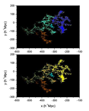
Figure 25: Two-dimensional map of the structures of the two largest coherent clusters detected from sample 1 when a brighter magnitude limit is adopted. The blue color stands for cluster 1 and the cyan color for cluster 2. The old galaxy members of the the two clusters are also presented for the sake of comparison, where the yellow color represents the old cluster 1 and the orange color denotes the old cluster 2.

Some authors proposed that the three dimensional topology of large-scale structures is spongelike (Gott III et al. 1986; Vogeley et al. 1994; Colley et al. 2000). Indeed, when plotting the structures of the two largest clusters identified from sample 1 in a lower resolution map, this type of feature emerges (see figure 25). It suggests that the large-scale structure of the local Universe is intrinsically coral-like, but it could also be spongelike if the resolution of the map is low enough.

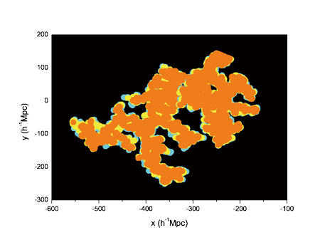
Figure 26: Low resolution (two-dimensional) map of the structures of the two largest coherent clusters identified from sample 1. The colors denoting different crowded sources are the same as they are coded in figure 6. For the definition of the coordinates, see figure 6.

As already pointed out by Gott III et al. (2005) that some larger structures are found if larger samples are involved. This is natural and is indeed observed in the analysis on sample 2, where the two large-scale structures detected in a smaller sample (sample 1) merge and a much larger structure is identified (see figure 22). (Accordingly, as the volume of sample 2 occupies only a small fraction of the nearby space, it is suspected that we might be able to observe a structure with its scale as large as $\sim 1000h^{-1}Mpc$ in the local Universe so long as the whole sky is surveyed.)

Implied by figure 21, some of the coherent clusters and unclustered sources seem to be able to connect with each other in a two-dimensional view. This is indeed true. When one repeats the above analysis on sample 1 under the condition that the contribution of the vertical length (i.e., the contribution of the coordinate $z$ defined in figure 6) is ignored, one identifies a much larger coherent cluster than the largest one obtained above (the details of the analysis are omitted). This suggests that some large-scale structures observed in a two-dimensional map might not be a coherent one when the vertical length is taken into account. As shown in Table 2, the mean redshift of cluster 1 is 0.0864. At this redshift, the vertical length confined by the adopted window of sample 1 (say, $-4.8^{\circ}<Dec.(J2000)<1.0^{\circ}$) is $25.7h^{-1}Mpc$, while the adopted criterion clustering scale at this redshift is $r_{ccs}=3.07h^{-1}Mpc$. The former is about 8 times of the latter. Keeping this in mind, the phenomenon that some structures connected in a two-dimensional map are in fact separated is expectable.

Note that $r_{ccs}$ might be different for different surveys. It is expected that the number of galaxies we will eventually ever be able to see would be larger than that observable today by a factor of $2.36$ (Gott III et al. 2005). If sample 1 is enlarged by two times, $r_{ccs}$ might probably shrink to a smaller scale. It is unnecessary that this would lead to a smaller scale of the largest structure identified with $r_{ccs}$. One reason is that the enlarging of the sample makes the sources more crowded and then separated sources are easier to be connected. Another reason is that the largest structure is constructed with the frames made up of very crowded sources (with several times of number density than that of the background data). The enlargement of the sample (only two times larger) would not be able to change this situation.

It should be pointed out that the structure scale as large as $357h^{-1}Mpc$ obtained from sample 1 and that as large as $659h^{-1}Mpc$ gained from sample 2 depend on the criterion clustering scale adopted in this paper, $r_{ccs}=[2\rho_{0}(z)]^{-1/3}$. It is obvious that when a smaller $r_{ccs}$ is adopted, then a smaller value of the largest structure scale identified from the samples would be obtained, and when a larger one is taken, then one would get a larger value of the largest structure scale. Thus, talking the largest structure scale one should refer to the corresponding criterion clustering scale. Due to this and due to the fact that the criterion clustering scale adopted in this paper varies with redshift, the comparison of the largest structure scale between our analysis and other previous ones has less meaning. It is desired that we can construct a standard criterion clustering scale one day and then can compare the largest structure scale obtained from various samples or from different regions of the Universe. Although we are unable to compare our results with others, the algorithm adopted in this paper tends to pick out larger structures than what identified previously, when similar criterion clustering scales are adopted. It is because that we are identifying large-scale structures in the co-moving frame of the Universe rather than in the observer frame. It is natural that those galaxies excluded in the previously identified large-scale structures due to their large redshifts are possible becoming members of some large-scale structures identified in this paper when they are located in a relatively dense region (see Fig. 22).

Martinez et al. (1998) searched for the scale of homogeneity by applying the $K$ function to galaxy catalogues. They detected the fingerprint of the transition to homogeneity in all the cases considered. Amendola & Palladino (1999) analyzed volume-limited subsamples of a redshift survey to search for the scale of homogeneity and found that the survey shows a trend of homogeneity at large scales. As shown in figure 4, one finds a trend toward homogeneity as well. We argue that, at least what revealed by figure 4 could not be interpreted as the existence of a transition to homogeneity at a large scale since that scale is comparable to the maximum scale of the adopted sample (see the caption of figure 4). As pointed out in Section 3, we suspect that the flux limit as well as the possible evolutionary effect might be the main factors that block the detection of the real scale of homogeneity. The previous methods cannot solve this problem, neither can the neighborhood function introduced in this paper. Only when this effect is removed, one will be able to determined the homogeneity scale with galaxy redshift surveys.

It may be an intrinsic property that this method naturally produces larger structures than other approaches do.

As suggested above, filamentary features are observed in the state of random distribution, formed by crowded sources (see figure 10). This is in agreement with the previous prediction that galaxies preferentially formed in large-scale filamentary or sheet-like mass overdensities in the early Universe, which was detected at as far as $z=3.1$ (Matsuda et al. 2005). When sorting out all sources of the background sample with $r_{ccs}$ we get many weak clusters and few less prominent clusters (see figure 15 panels d and f). According to definition, these clusters are likely the so-called protoclusters (Venemans 2005). The latter were identified at $z\sim 4$ in recent observations (Venemans et al. 2002; Miley et al. 2004; Intema et al. 2006).

According to the above analysis we conclude that: 1) the probability of forming the large-scale structures, detected from sample 1 with our method, by chance is very small; 2) the phenomenon of clustering is dominant in the local Universe; 3) coherent clusters with the scale as large as $357h^{-1}Mpc$ and the number of galaxies as large as 12966 are identified from sample 1 well within the $3\sigma$ confidence level; 4) there exist some galaxies which are not affected by the gravitation of clusters and therefore are likely to rest on the co-moving frame of the Universe; 5) filamentary features could appear in the state of random distribution; 6) voids are likely the volumes within which no very crowded sources are present and they are likely formed in embryo by fluctuation in the very early epoch of the Universe and it might be the continuous gravitation in later time that pulls crowded galaxies closer and in the same time leaves behind adult voids; 7) large-scale structures are coral-like and they are likely made up of smaller ones and in forming the former the latter are likely connected by their antennae; 8) very crowded sources are mainly distributed within the structure of prominent clusters and it is them who form the frame of the large-scale structure.

Table 1: Description of samples.

name	number	area	regiona	$\rho_{0}(z)$c	data
sample 1	59497	$150.0^{0}<RA<220.0^{0}$	NGP	$\rho 1$	observation
		$-4.8^{0}<DEC<1.0^{0}$
sample 2	226302	The whole area of the 2dF survey	NGP, SGPb	$\rho 1$	observation
sample 3	59497	That of sample 1	NGP	$\rho 1$	simulation
sample 4	59497	That of sample 1	NGP	$\rho 2$	simulation
sample 5	59497	That of sample 1	NGP	$\rho 3$	simulation

a: For definitions of NGP and SGP, see Colless et al. (2001).
b: In addition to NGP and SGP, sample 2 covers all other ‘random’ fields of the 2dF survey.
c: In this column we list the $\rho_{0}(z)$ that is used to perform the corresponding simulations, to calculate the corresponding $\kappa$, and/or to determine the corresponding $r_{ccs}$, where $\rho 1$ is that directly measured from sample 2, $\rho 2$ is the polynomial function obtained by a fit to $\rho 1$, and $\rho 3=\rho_{0}=0.00247(Mpc/h)^{-3}$ is a constant.

Table 2: Parameters of the $67$ coherent clusters with $P<P(3\sigma)$ detected from sample 1.

label	number	$\kappa(r_{ccs})$	scalea	$\overline{z}$	label	number	$\kappa(r_{ccs})$	scale	$\overline{z}$
1	12966	6.04	281	0.0864	35	128	4.73	12.0	0.0238
2	7788	4.07	357	0.136	36	121	2.82	34.2	0.136
3	4216	7.24	136	0.0485	37	121	1.79	106	0.218
4	2100	4.24	177	0.130	38	118	2.11	71.5	0.201
5	1215	3.78	112	0.124	39	103	3.27	56.2	0.184
6	922	3.56	127	0.173	40	102	3.82	58.4	0.185
7	805	5.56	51.9	0.0533	41	98	4.22	19.5	0.0790
8	668	3.93	62.5	0.111	42	97	2.84	29.6	0.105
9	615	3.29	121	0.182	43	95	2.92	26.4	0.0958
10	540	3.96	56.6	0.0748	44	95	3.18	26.4	0.0829
11	448	3.22	46.7	0.0821	45	82	9.29	13.1	0.0086
12	401	2.97	125	0.167	46	81	4.24	15.9	0.0175
13	369	6.45	28.7	0.0264	47	79	6.73	0.714	0.0005
14	349	14.5	0.343	0.0001	48	79	3.88	28.8	0.108
15	348	6.70	26.3	0.0236	49	78	5.17	16.8	0.0759
16	333	9.34	0.688	0.0002	50	74	4.73	22.8	0.100
17	321	3.16	70.6	0.166	51	70	3.39	58.2	0.200
18	287	5.56	26.1	0.0476	52	63	3.72	0.512	0.0004
19	280	3.48	68.2	0.105	53	62	3.78	12.4	0.0304
20	271	3.74	89.8	0.189	54	59	4.25	1.09	0.0006
21	269	3.95	59.9	0.103	55	56	3.78	25.9	0.107
22	257	7.52	0.900	0.0003	56	55	3.46	23.7	0.115
23	228	4.37	24.1	0.0203	57	53	4.08	8.54	0.0044
24	218	5.70	18.7	0.0201	58	51	3.74	40.3	0.214
25	216	2.86	92.1	0.150	59	47	4.23	12.4	0.0535
26	211	3.51	64.6	0.145	60	40	4.42	13.6	0.100
27	194	3.21	32.6	0.0475	61	31	4.61	0.477	0.0007
28	188	3.46	56.6	0.144	62	29	6.21	8.96	0.103
29	182	3.77	52.4	0.132	63	25	4.27	9.30	0.0654
30	175	3.90	40.3	0.0689	64	22	4.59	0.320	0.0006
31	155	3.58	55.1	0.165	65	22	4.31	10.7	0.141
32	154	4.28	23.4	0.0648	66	15	6.39	7.51	0.147
33	139	5.43	0.823	0.0004	67	11	5.69	7.47	0.125
34	133	3.72	39.6	0.136

a: in units of $h^{-1}Mpc$.

References

- [1]
- [2] []Amendola, L. & Palladino, E. 1999, ApJ, 514, L1
- [3]
- [4] []Bahcall, N. A., & Soneira, R. M. 1983, ApJ, 270, 20
- [5]
- [6] []Bagchi, J., Enlin, T. A., Miniati, F. et al. 2002, New Astron., 7, 249
- [7]
- [8] []Benson, A. J., Cole, S., Frenk, C. S., Baugh, C. M., & Lacey, C. G. 2000, MNRAS, 311, 793
- [9]
- [10] []Benson, A. J., Frenk, C. S., Baugh, C. M., Cole, S. & Lacey, C. G. 2001, MNRAS, 327, 1041
- [11]
- [12] []Berlind, A. A., Weinberg, D. H., Benson, A. J., Baugh, C. M., Cole, S., Davé, R., Frenk, C. S., Jenkins, A., Katz, N., & Lace, C. G. 2003, ApJ, 593, 1
- [13]
- [14] []Bharadwaj, S., Sahni, V., Sathyaprakash, B. S., Shandarin, S. F., & Yess, C. 2000, ApJ, 528, 21
- [15]
- [16] []Bhavsar, S. P., & Ling, E. N. 1988, ApJ, 331, L63
- [17]
- [18] []Blumenthal, G. R., Faber, S. M., Primack, J. R., & Rees, M. J. 1984, Nature, 311, 517
- [19]
- [20] []Cannon, R., Drinkwater, M., Edge, A. et al. 2006, MNRAS, 372, 425
- [21]
- [22] []Cembranos, J. A. R., Feng, J. L., Rajaraman, A. & Takayama, F. 2005, PRL, 95, 1301
- [23]
- [24] []Cen, R., & Ostriker, J. P. 2000, ApJ, 538, 83
- [25]
- [26] []Coil, A. L. et al., 2004, ApJ, 609, 525
- [27]
- [28] []Colberg, J., Krughoff, S., & Connolly, A. 2005, MNRAS, 359, 272
- [29]
- [30] []Coleman, P. H., Pietronero, L., & Sanders, R. H. 1988, A&A, 200, L32
- [31]
- [32] []Colless, M. et al., 2001, MNRAS, 328, 1039
- [33]
- [34] []Colless, M. et al., 2003, Preprint (astro-ph/0306581)
- [35]
- [36] []Colley, W. N., Gott, III. J. R., Weinberg, D. H., Park, C., & Berlind, A. A. 2000, ApJ, 529, 795
- [37]
- [38] []Cross, N. J. G., Driver, S. P., Liske, J. et al., 2004, MNRAS, 349, 576
- [39]
- [40] []Davis, M., & Geller, M. J. 1976, ApJ, 208, 13
- [41]
- [42] []Davis, M., & Peebles, P. J. E. 1983, ApJ, 267, 465
- [43]
- [44] []Davis, M., Efstathiou, G., Frenk, C. S., & White, S. D. M. 1985, ApJ, 292, 371
- [45]
- [46] []Davis, M., Efstathiou, G., Frenk, C. S., & White, S. D. M. 1992, Nature, 356, 489
- [47]
- [48] []Deng, X. F., Chen, Y. Q., Zhang, Q., & He, J. Z. 2006, ChJAA, 6, 35
- [49]
- [50] []Diaz, E., Zandivarez, A., Merchan, M. E., & Muriel, H. 2005, ApJ, 629, 158
- [51]
- [52] []Diggle, P. J. 1983, Statistical Analysis of Spatial Point Patterns (London: Academic Press)
- [53]
- [54] []Doguwa, S. I., & Upton, G. J. G. 1989, BIOM. J., 5, 563
- [55]
- [56] []Ebeling, H., Barrett, E., & Donovan, D. 2004, ApJ, 609, L49
- [57]
- [58] []Einasto, J., Klypin, A. A., Saar, E., & Shandarin, S. F. 1984, MNRAS, 206, 529
- [59]
- [60] []Einasto, J., & Gramann, M. 1993, ApJ, 407, 443 443
- [61]
- [62] []Einasto, J. et al., 2006a, Preprint (astro-ph/0603764)
- [63]
- [64] []Einasto, J. et al., 2006b, Preprint (astro-ph/0604539)
- [65]
- [66] []Eke, V. R. et al., 2004, MNRAS, 348, 866
- [67]
- [68] []Erdogdu, P. et al., 2004, MNRAS, 352, 939
- [69]
- [70] []Feldman, H. A., Kaiser, N., & Peacock, J. A. 1994, ApJ, 426, 23
- [71]
- [72] []Fisher, K. B., Davis, M., Strauss, M. A., Yahil, A., & Huchra, J. P. 1993, ApJ, 402, 42
- [73]
- [74] []Gellar, M. J., & Huchra, J. 1989, Science, 246, 897
- [75]
- [76] []Gott, III. J. R., Dickinson, M., & Melott, A. L. 1986, ApJ, 306, 341
- [77]
- [78] []Gott, III. J. R., Juric, M., Schlegel, D., Hoyle, F., Vogeley, M,, Tegmark, M., Bahcall, N., & Brinkmann, J. 2005, ApJ, 624, 463
- [79]
- [80] []Governato, F., Baugh, C. M., Frenk, C. S., Cole, S., Lacey, C. G., Quinn T., & Stadel, J. 1998, Nature, 392, 359
- [81]
- [82] []Guzzo, L. 2002, in Dark matter in astro- and particle physics, Proc. of the Int. Conf. DARK 2000, ed H. V. Klapdor-Kleingrothaus and R. D. Viollier (Springer), p 3, Preprint ( astro-ph/0207285)
- [83]
- [84] []Hawkins, E. et al., 2003, MNRAS, 346, 78
- [85]
- [86] []Haynes, M. P., & Giovarelli, R. 1986, ApJ, 306, L55
- [87]
- [88] []Hoyle, F., Vogeley, M. S., Gott, III. J. R., Blanton, M., Tegmark, M., Weinberg, D. H., Bahcall, N., Brinkmann, J., & York, D. 2002, ApJ, 580, 663
- [89]
- [90] []Huchra, J. P., & Geller, M. J. 1982, ApJ, 257, 423
- [91]
- [92] []Intema, H. T., Venemans, B. P., Kurk, J. D., Ouchi, M., Kodama, T., Rottgering, H. J. A., Miley, G. K., & Overzier, R. A. 2006, A&A, in press, Preprint (astro-ph/0606298)
- [93]
- [94] []Jing, Y. P., & Zhang, J. L. 1988, A&A, 190, L21
- [95]
- [96] []Joyce, M., Montuori, M., & Sylos, L. F. 1999, ApJ, 514, L5
- [97]
- [98] []Joyce, M., Sylos, L. F., Gabrielli, A., Montuori, M., & Pietronero, L. 2005, A&A, 443, 11
- [99]
- [100] []Kaiser, N. 1987, MNRAS, 227, 1
- [101]
- [102] []Kauffmann, G., Colberg, J. M., Diaferio, A., & White, S. D. M. 1999, MNRAS, 307, 529
- [103]
- [104] []Kirshner, R. P., Oemler, A. J., Schechter, P. L., & Shectman, S. A. 1981, ApJ, 248, L57
- [105]
- [106] []Lahav, O., & Suto, Y. 2004, LIVING REV. RELATIVITY, 7, 8
- [107]
- [108] []Loveday, J., Efstathiou, G., Peterson, B. A., & Maddox, S. J. 1992, ApJ, 400, L43
- [109]
- [110] []Lynden-Bell, D., Faber, S. M., Burstein, D., Davies, R. L., Dressler, A., Terlevich, R. J., & Wegner, G. 1988, ApJ, 326, 19
- [111]
- [112] []Martinez, V. J., Pons-Borderia, M.-J., Moyeed, R. A., & Graham, M. J. 1998, MNRAS, 298, 1212
- [113]
- [114] []Martinez, V. J., Lopez-Marti, B., & Pons-Borderia, M.-J. 2001, ApJ, 554, L5
- [115]
- [116] []Martinez, V. J., & Saar, E. 2002a, in the proc. of “Statistical Challenges in Modern Astronomy III”, ed G. J. Babu and E. D. Feigelson (Springer), Preprint (astro-ph/0203251)
- [117]
- [118] []Martinez, V. J., & Saar, E. 2002b, Astronomical Data Analysis II, ed J.-L. Starck and F. D. Murtagh, Proc. of the SPIE, 4847, p86, Preprint (astro-ph/0209208)
- [119]
- [120] []Matsuda, Y. et al., 2005, ApJ, 634, L125
- [121]
- [122] []Merchan, M. E., Maia, M. A. G., & Lambas, D. G. 2000, ApJ, 545, 26
- [123]
- [124] []Merchan, M. E., & Zandivarez, A. 2005, ApJ, 630, 759
- [125]
- [126] []Miley, G. K. et al., 2004, Nature, 427, 47
- [127]
- [128] []Norberg, P., Cole, S., Baugh, C. M. et al., 2002, MNRAS, 336, 907
- [129]
- [130] []Ouchi, M. et al., 2005, ApJ, 620, L1
- [131]
- [132] []Padilla, N. D. et al., 2004, MNRAS, 352, 211
- [133]
- [134] []Park, C., Vogeley, M. S., Geller, M. J., & Huchra, J. P. 1994, ApJ, 431, 569
- [135]
- [136] []Patiri, S. G., Prada, F., Holtzman, J., Klypin, A., & Betancort-Rijo, J. 2006, Preprint (astro-ph/0605703)
- [137]
- [138] []Peebles, P. J. E. 1974, ApJ, 189, L51
- [139]
- [140] []Peebles, P. J. E. 1980, The Large-Scale Structure of the Universe (Princeton: Princeton Univ. Press)
- [141]
- [142] []Peebles, P. J. E. 1982, ApJ, 263, L1
- [143]
- [144] []Pimbblet, K. A., Smail, I., Edge, A. C. et al., 2001, MNRAS, 327, 588
- [145]
- [146] []Pimbblet, K. A., Drinkwater, M. J., & Hawkrigg, M. C. 2004 MNRAS, 354, L61
- [147]
- [148] []Porter, S. C., & Raychaudhury, S. 2005, MNRAS, 364, 1387
- [149]
- [150] []Ripley, B. D. 1981, Spatial Statistics (New York: John Wiley & Sons)
- [151]
- [152] []Rivolo, A. R. 1986, ApJ, 301, 70
- [153]
- [154] []Schlegel, D. J., Finkbeiner, D. P., & Davis, M. 1998, ApJ, 500, 525
- [155]
- [156] []Seldner, M., Siebers, B., Groth, E. J., & Peebles, P. J. E. 1977, ApJ, 82, 249
- [157]
- [158] []Shimasaku, K. et al., 2003, ApJ, 586, L111
- [159]
- [160] []Steidel, C. C., Adelberger, K. L., Dickinson, M., Giavalisco, M., Pettini, M., & Kellogg, M. 1998, ApJ, 492, 428
- [161]
- [162] []Tadros, H., & Efstathiou, G. 1996, MNRAS, 282, 1381
- [163]
- [164] []Totsuji, H., & Kihara, T. 1969, PASJ, 21, 221
- [165]
- [166] []Vasilyev, N. L., Baryshev, Y. V., & Sylos, L. F. 2006, A&A, 447, 431
- [167]
- [168] []Venemans, B. P. et al., 2002, ApJ, 569, L11
- [169]
- [170] []Venemans, B. P. 2005, Ph.D. thesis (Leiden: Sterrewacht, Leiden University)
- [171]
- [172] []Vogeley, M. S., Park, C., Geller, M. J., Huchra, J. P., & Gott, III. J. R. 1994, ApJ, 420, 525
- [173]
- [174] []Yadav, J., Bharadwaj, S., Pandey, B., & Seshadri, T. R. 2005, MNRAS, 364, 601
- [175]
- [176] []York, D. G. et al., 2000, AJ, 120, 1579
- [177]
- [178] []Yoshida, N. et al., 2001, MNRAS, 325, 803
- [179]
- [180] []Yoshida, N. 2005, Prog. Theor. Phys. Suppl., 158, 117
- [181]
- [182] []Zandivarez, A., Merchan, M. E., & Padilla, N. D. 2003, MNRAS, 344, 247
- [183]
- [184] []Zehavi, I. et al., 2002, ApJ, 571, 172