Phase Space Structure in the Solar Neighbourhood

Abstract

Aims. To examine the idea that dynamical parameters can be estimated by identifying locations in the solar neighbourhood where velocity distributions recovered from test particle simulations, match the observed local distribution. Here, the dynamical influence of both the Galactic bar and the outer spiral pattern are taken into account.

Methods. The Milky Way disc is stirred by analytical potentials that are chosen to represent the two perturbations, the ratio of pattern speeds of which is explored, rather than held constant. The velocity structure of the final configuration is presented as heliocentric velocity distributions at different locations. These model velocity distributions are compared to the observed distribution in terms of a goodness-of-fit parameter that has been formulated here. We monitor the spatial distribution of the maximal value of this goodness-of-fit parameter, for a given simulation, in order to constrain the solar position from this model. Efficiency of a model is based on a study of this distribution as well as on other independent dynamical considerations.

Results. We reject the bar only and spiral only models and arrive at the following bar parameters from the bar+spiral simulations: bar pattern speed of 57.4${}^{+2.8}_{-3.3}$ km s^-1 kpc^-1and a bar angle in [0^∘, 30^∘], where the error bands are $\pm$1-$\sigma$. However, extracting information in this way is no longer viable when the dynamical influence of the spiral pattern does not succumb to that of the bar; an explanation for this is offered. Orbital analysis indicates that even though the basic bimodality in the local velocity distribution can be attributed to scattering off the Outer Lindblad Resonance of the bar, it is the interaction of irregular orbits and orbits of other resonant families, that is responsible for the other moving groups; it is realised that such interaction increases with the warmth of the background disk.

1 Introduction

Historically, stars in the solar neighbourhood were considered to exhibit purely random peculiar motion; guided by this notion, the motion of the Sun was calculated from chosen stellar samples. This idea was challenged by Jacob Kapteyn at the beginning of the last century when he observed preferential stellar motion in two favoured directions. Within the next few decades, the situation was realised to be more complicated, though the dominance of the two Kapteyn streams (Stream I $\&$ II) was established. The apex of the motion of the stars in Stream I was observed to correspond to the convergent point of the proper motions of the Hyades cluster (Eggen 2004) while that of the members in Stream II almost coincides with the convergent point of proper motions of the Sirius supercluster. Thus Stream I is also referred to as the Hyades stream, while Stream II is referred to as the Sirius stream. As observations improved, more moving groups were observed in the solar neighbourhood, such as the Hercules, Coma Berenices and Pleiades streams, (Fux 2000).

In the past, work has been done to understand the origin of the moving groups in the solar neighbourhood, as handiwork of the bar or transient spirals (Dehnen 2000; Fux 2001; de Simone et. al 2004; Quillen 2003; Quillen & Minchev 2005). But no such exercise took into account the joint effect of these two disc structures, while scanning through a possible range of the ratio of their pattern speeds. This ratio is foreseen to have serious dynamical influence in sculpting the local phase space. Such modelling is included in this paper.

Also, while work has been done to estimate the bar parameters (pattern speed and bar angle) from a comparison of simulated velocity distributions $f_{s}$ and the observed velocity distribution $f_{o}$ (Dehnen 2000), a rigorously quantified comparison of the same has not been carried out. This obviously hinders the possibility of scanning through an assortment of models and also renders such parameter estimates subjective. In this paper, a statistical formalism is presented that allows for such objective comparison. In fact, this methodology points to the fallibility of attempting to extract dynamical parameters from such comparison, in cases when the influence of the spiral is strong.

Additionally, multiple suggestions appear to have been put forward toward a dynamical origin for the moving groups. In Kalnajs (1991), it was argued that if the Outer Lindblad Resonance due to the central bar ($OLR_{b}$) in our Galaxy corresponded roughly to the solar radius, then an observer at the Sun would be close to the point of intersection of the aligned and anti-aligned orbits that lie on either side of the resonance location and identify the local stellar distribution as bimodal, (Fig 1). This bimodality was also picked up by Palous $\&$ Hauck (1986) in a paper that reported the distribution of a sample of A-type stars in the solar neighbourhood. In Dehnen (2000), results of simulations done (by backward integration) with a central bar imposed on a disk, were reported; it was concluded that the bar angle lies in the range [$10^{\circ},70^{\circ}$] and the bar pattern speed is $53\pm 3$ km s^-1 kpc^-1. This value falls slightly short of $59\pm 2$ km s^-1 kpc^-1that is suggested for the bar pattern speed in the hydrodynamical work by Englmaier & Gerhard (1999) but falls within the range suggested in an application of the Tremaine-Weinberg method to a sample of OH/IR stars in our Galaxy by Debattista et al. (2002) - $59\pm 5$ km s^-1 kpc^-1with a possible systematic error of 10 km s^-1.

Fux (2000) discusses the results of a high-resolution N-body simulation aimed at investigating barred models of the Galaxy. The local velocity distribution function was smoothed by the adaptive kernel smoothing technique discussed in Skuljan et. al (1999). It is to be noted that this sample is biased since the used radial velocities are for the high proper motion stars only (Binney et. al 1997; Skuljan et. al 1999; Fux 2001). Nonetheless, stellar streams are distinctly visible in this distribution as well as in the model distributions recovered by Fux. According to Fux, $R_{\rm OLR}=7.7$ kpc and the bar angle is $25^{\circ}$. Figure 2 represents the local velocity distribution, as estimated in Fux (2000). The velocity data corresponding to this figure and the smoothing algorithm used to deduce the contour plot presented therein, were very kindly supplied by R.Fux.

The observed bimodality in the velocity distribution in the solar neighbourhood has been explained in Fux (2000) along the same lines as in Raboud et. al (1998). The Jacobi integral, in the rotating frame of the bar, is stationary at five Lagrange points on a zero-velocity surface; these five characteristic values of the integral correspond to two maxima, one minima and the two saddle points, in the effective potential. If the Jacobi energy of a star exceeds the value of the effective potential that characterises the saddle points, then the star is free to cross corotation and escape to infinity, (in principle). Following Fux (2000), such stars are said to be on “hot” orbits. The Hercules stream is concluded to be due to stars on such orbits. The stability of the orbits is dealt with in details in Fux (2001); in this work, the Hercules stream is proposed to be due to an overdensity of chaotic orbits at spatial locations that are near or just outside the OLR.

de Simone et. al (2004) propose the heating of the disk by strong transient spiral waves as the source of the moving groups that are evident in the local phase space structure. They also suggest that this mechanism can explain the observation that ages of the stars in the same moving group vary over a wide range. Famaey et. al (2005) agree that this wide variation of ages within the same moving group can be understood as due to the migration of stars from an original galactocentric location, brought about by a transient spiral wave and that the streams are dynamical in origin and not derivatives of irregularities in the star formation rate.

Quillen (2003) deals with the case of the perturbation due to a bar and a spiral pattern, as was investigated in Paper I. From the mapping of the phase space via Poincare maps, Quillen (2003) realised that the quasi-periodic orbits that support the bar and the spiral structure, are disrupted around the OLR of the bar when the solar radius just exceeds the location of the ILR of the spiral pattern. Quillen & Minchev (2005) attribute the splitting of the Hyades-Pleiades group to spirality.

Chakrabarty (2004) (hereafter Paper I) reported a series of direct two dimensional test particle simulations in which the outer parts of different disk configurations (cold Mestel and warm quasi-exponential) were stirred by non-axisymmetric perturbations due to the bar alone, a spiral pattern alone, and the bar and the spiral acting in concert. The result of the perturbation was gauged via the distributions in the space of the heliocentric radial velocities ($U$) and tangential velocities ($V$), disk heating and spatial re-arrangement of the stars in the disc. The effects of growing and subsequently dissolving a perturbation were also looked into.

While in Paper I we attempted to understand the general perturbative effects of non-axisymmetric features, in this paper, such an investigation is configured to model the effects of the Galactic bar and outer spiral pattern on the phase space distribution in the vicinity of the Sun.

The paper has been organised as follows. In the following section, we discuss the methodology that is used here. In Section 3, we elucidate the basic parameters used in our models and introduce the goodness-of-fit statistic that we use. In Section 4, velocity distributions obtained from our simulations have been presented at various locations, for the different runs that have been performed. An analysis of some orbits responsible for the main structures observed in the velocity space is presented in Section 5. We then proceed to discuss some of the issues that the results alluded to, in Section 6. The paper is rounded up with a short summary of the main results.

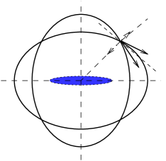
Figure 1: The OLR location is marked by orbits of opposite orientations on either side of the resonance; orbits are aligned with the major axis of the bar just outside the resonance while just inside, circular orbits are distorted into anti-aligned shapes. The local velocity distribution, as viewed by an observer sitting at the junction of these two different orbits, is bimodal. The bar is shown by the solid ellipse at the centre.

2 Method

In this paper, we undertake an exercise similar to that in Paper I, but configure the structures to a model for the Milky Way disc. The initial positions of the stars are extracted from a model for the disk (discussed below) and the orbits are numerically integrated in the potential of the background disk, on which is imposed the analytical potential of the model Galactic bar and/or the outer spiral pattern. The spatial band under investigation is put on a regular polar grid. At each $R-\phi$ cell in this grid, the resulting orbits are put on a regular Cartesian $U-V$ grid. The velocity distribution recovered at an $R-\phi$ cell is compared to the observed local $U-V$ distribution (Figure 2). If the comparison is favourable, the corresponding $R-\phi$ location is branded “good”. A rigorous statistical formalism to evaluate the quality of this comparison is presented below. Thus, a model velocity distribution is “good” if it corresponds to a high value of the goodness of fit index.

The spatial distribution of these “good” locations are then used to constrain the solar position, which is subsequently implemented to estimate relevant dynamical parameters, such as the bar angle and the bar pattern speed. (In our scale free disk, we express all lengths in units of the corotation radius $R_{\rm CR}$ of the bar. Thus, identifying the solar radius enables us to scale all lengths to real units; given that the bar pattern speed determines $R_{\rm CR}$, the scaling implies constraining the bar pattern speed.)

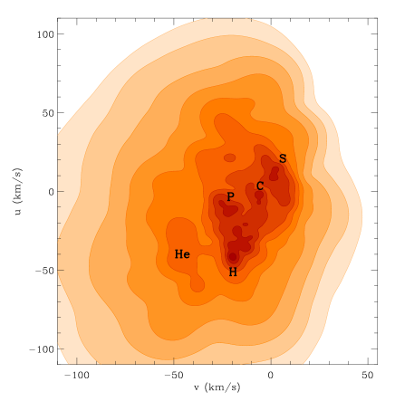
Figure 2: The solar neighbourhood distribution diagram produced with the velocity data and smoothing code, shared with us by Fux. The distribution above differs from Figure 1 in Fux (1999) in the definition of the direction of positive $U$, (towards Galactic centre in the figure above). $V$ is positive in the sense of Galactic rotation. The above distribution is built from the transverse velocities of Hipparcos single stars with distance $d<100$pc, dispersion of parallax $\sigma(\pi)<0.1\pi$ from the Hipparcos Catalogue and with radial velocities of the 3481 stars in the Hipparcos Input Catalogue. Logarithmic contours have been used.

3 Simulation Background

Here we discuss some of the salient features of our simulations.

3.1 Models

The models that we have used in our simulations are typically characterised by two classes of parameters: disk and perturber. An important feature of the perturbing potential is the strength parameter; this is the ratio of the field due to the imposed perturber at a chosen radius, (namely the OLR due to an $m=2$ perturbation in a Mestel potential) to the field due to the background disc. Additionally, the simulations that include the spiral pattern, are distinguished from each other in terms of the choice of the ratio of the pattern speed of the spiral to the bar. The other parameters of the spiral pattern, such as the number of arms and pitch angle are held a constant.

The observational milieu that inspires the choice of the values of these parameters is discussed below.

1. The Galactic disk was modelled to have a uniform rotation curve, (Mestel 1963) and an almost exactly exponential surface density profile with a scale length of about 0.9$R_{\rm CR}$. This was ensured by characterising the disk with the doubly cut-out equilibrium stellar distribution function, discussed in Evans $\&$ Read (1998); Evans (1994) and used extensively in Paper I. At the end of each simulation, the radial and azimuthal velocity dispersions ($\sigma_{U}$ and $\sigma_{V}$), and the vertex deviation ($l_{v}$) are noted at different locations within the annulus that we study. These quantities should reflect observations on a typical eclectic sample of stars in the solar neighbourhood (Table 10.2 in (Binney $\&$ Merrifield 1998)). The values of $\sigma_{U}$, $\sigma_{V}$ and $l_{v}$ are included in Table 1, which represents the results from the runs performed with the different models. Thus, we strive to ensure that the state of the background disk abides by relevant observations. On the other hand, the state of the disk at time $t=0$ may have been very different; after all, disk characteristics prior to the growth of the Galactic bar (and/or outer spiral) are not known to us. Thus, any model that offers the correct final configuration, suffices. The $\sigma_{U}$ of the model disk at $t=0$ is about 21 kms^-1 while the value of the Oort ratio in the initial disk is about 0.67.

2. This equilibrium model is perturbed either by a quadrupolar bar or a logarithmic outer spiral pattern, or simultaneously by both these features. Thus, in the frame that is stationary with the bar, the bar potential is (as given by Equation 10 in Paper I):

   $$\Psi_{\rm bar}=\epsilon\displaystyle{\frac{\cos(2\phi)}{R^{3}}}$$ (1)

   Now Dehnen (1999) suggests that at the solar radius ($R_{\odot}$), the amplitude of $\Psi_{\rm bar}$ is about 0.036$v_{0}^{2}R_{\rm CR}^{3}/R_{\odot}^{3}$, where $v_{0}$ is the amplitude of the rotation curve at the solar circle. Now, as in Paper I, we work in a scale free Mestel disk, in which, $v_{0}$=1 and $R_{\rm CR}$=1, (this $R_{\rm CR}$ follows from the setting of the bar pattern speed to unity). Connecting our strength parameter to the strength used by Dehnen (1999), we get: $\epsilon\approx$0.036$v_{0}^{2}R_{\rm CR}^{3}$. Now Fux (2001) works with bars that are double in strength. We choose to adopt the middle path by working with a bar that has an average of the strengths implemented by Fux (2001) and Dehnen (1999). This implies that the ratio of the gravitational field of the bar to that of the background disk is about 3.6$\%$, at the OLR.

3. The outer spiral pattern is chosen to have 4-arms and a pitch angle of $15^{\circ}$. Vallee (2002) provides a comprehensive review of the parameters pertinent to the Galactic spiral pattern. This review suggests that the pitch angle lies in the range of 6^∘ to 17^∘, with the mean around 12^∘. We work with a pitch angle of 15^∘, more along the lines of Johnston et. al (2001), who also suggest a 4-armed pattern. These many arms are compatible with the best-fitting (“standard”) model of the Galactic spiral pattern in the work by Bissantz et. al (2003). Block & Puerari (1999) looked at the $K$-band spiral structure of a sample of 19 galaxies and concluded that the fractional amplitude with respect to the background disk of an $m$=2 spiral ranges from 0.03 to 0.5, with the median at 0.1. Now, the amplitude of an $m$-armed spiral pattern goes as $1/m$ ((de Simone et. al 2004)). Thus, the range allowed for the fractional amplitude of the 4-armed spiral, according to Block & Puerari (1999) is 0.015 to 0.25, with a median at 0.05. We choose to work with a 4-armed spiral that has a fractional amplitude of 0.036. Our spiral strength is therefore on the weaker side.

4. When the bar and the spiral pattern are imposed on the disk together, the chosen amplitude for the perturbation field, (at $OLR_{b}$), is about $4.9\%$ of the field of the background disk, in which, the contributions of the bar to the spiral is in the ratio of 0.043:0.023.

5. As discussed in Paper I, the perturbation is imposed after the stars had experienced the axisymmetric Mestel potential for 80$\tau_{b}$/2$\pi$, where $\tau_{b}$ is the time taken for one bar revolution. The perturbation was then allowed to grow adiabatically to its maximum strength. By this we mean that the growth time is much larger than the dynamical time of the perturber. We chose the growth times of the bar and the spiral pattern to be equal (40$\tau_{b}$/2$\pi$). Orbits were recorded once the perturber strength had saturated to its maximum.

6. In the disk, a radial band is examined for the effects of the perturbations. The inner edge of this annulus is at $OLR_{b}$ and it extends outwards; specifically, radius ranges from $R/R_{\rm CR}=1.7$ to $R/R_{\rm CR}=2.3$. At the end of the simulation, the orbital position coordinates ($R$ and azimuth $\phi$, where $\phi$=0 is along the bar major axis) are placed on a regular $R-\phi$ grid and the velocity distributions of the stars lying in each $R-\phi$ cell is sought. In our simulations the extent of each radial cell is $R/R_{\rm CR}=0.025$. Therefore, any radial location, in units of $R_{\rm CR}$, is expressed with multiple significant figures. The azimuthal range under study is [$0^{\circ},360^{\circ}$] and any two azimuthal cells are $10^{\circ}$ apart. In the presentations of the results, we limit ourselves to the first quadrant in $\phi$ only.

7. The Hercules stream consists of stars at large negative tangential velocities. Such stars are on prograde orbits and must therefore have their guiding centres inside the solar circle. Thus, the way to boost the Hercules stream is to ensure that more stars from the inner disk are allowed to enter the annulus being studied. This can be controlled via the choice of the pattern speed of the spiral that is used in the simulation as is explained in the next paragraph. Of course, the surface density of the background disk will also contribute to this, but this is fixed since we work with a fixed background configuration (that has been ascribed an exponential profile).

8. We chose to work with a pattern speed for the spiral pattern that is distinct from that of the bar. Rautiainen $\&$ Salo (1999) have suggested N-body models in which the inner spiral rotates with the bar while the outer spiral is decoupled from it. Bissantz et. al (2003) have picked up on this theme to explore gas dynamical models of the galaxy, in which the bar and the outer spiral rotate with pattern speeds of about 60kms^-1kpc^-1 and 20kms^-1kpc^-1 respectively. Melnik (2006) too advocates a similar picture, with the Cygnus arm as the link between the inner (faster of the two patterns) and the outer spiral pattern. In fact, Melnik (2006) constrains the angular speed of the outer spiral pattern ($\Omega_{\rm sp}$) from the top by requiring that the Perseus arm be inside the corotation due to this pattern, i.e. $\Omega_{\rm sp}$ $<$ 25kms^-1kpc^-1. We take our cue from this suggestion and choose to work with three pattern speeds for the outer spiral: 18kms^-1kpc^-1, 21kms^-1kpc^-1 and 25kms^-1kpc^-1. When the 4:1 ILR due to our 4-armed spiral pattern ($ILR_{s}$) is constrained to approximately coincide with the location of $OLR_{b}$, it implies that $\Omega_{\rm bar}:\Omega_{\rm sp}=55:21$. In the other two cases, $ILR_{s}$ lies well inside the $OLR_{b}$ ($\Omega_{\rm bar}:\Omega_{\rm sp}=55:25\>\Longrightarrow\>R/R_{\rm CR}\approx$ 1.42) while in the other, $ILR_{s}$ is beyond $OLR_{b}$ and is located at $R/R_{\rm CR}\approx$ 1.97, ($\Omega_{\rm bar}:\Omega_{\rm sp}$=55:18). This radial location sits almost in the middle of the annular region of the disk that we investigate in our work. Thus in the first case, stars would be pushed into the radial range under investigation, since the ILR due to a spiral pattern is an “emitter” of angular momentum (Lynden-Bell $\&$ Kalnajs 1972). For this same reason, in the second case, the effect of the spiral pattern would be to deplete the immediate neighbourhood of the ILR, i.e. a part of the radial range under investigation. Thus in the light of the previous paragraph, this implies that when $ILR_{s}$ is chosen to lie inside the inner edge of the radial zone of investigation, the Hercules stream will be more populous than when the ILR is anywhere inside this zone.

3.2 Comparison

The solar neighbourhood $U-V$ velocity distribution $f_{o}$ is generated by Fux (2000) from the observed data by implementing the adaptive kernel algorithm suggested by Skuljan et. al (1999) (Figure 2). The simulated velocity distributions $f_{s}$ that we obtain at different observer locations, are similarly smoothed and then compared against the observed distribution.

To ensure that this comparison is not affected by any extraneous factors such as differences in the generation or representation of the (simulated or observed) distributions from the respective data sets, it was imperative that the model data be smoothed in the same way as the observed data. This was done by using the same adaptive kernel smoothing routine that Fux used.

The comparison between $f_{s}$ and $f_{o}$ is carried out in terms of a rigorous “goodness-of-fit” statistic (Section 3.3). Here are a few points to remember in regard to these comparisons.

• In making the comparison at any given $R-\phi$ address, we focus upon the 5 moving groups that have been marked in Figure 2- $f_{s}$ is identified as “good” if the locations of all the 5 groups in the $U-V$ plane match the $U-V$ coordinates of the corresponding groups in $f_{o}$.

• The match is considered acceptable within error bars that are given by the solar peculiar velocities ($|{V_{\odot}}|\approx$5 km s^-1and $|{U_{\odot}}|\approx$10 km s^-1). It needs to be emphasised that at any given $R,\phi$ location, the sub $U_{\odot}-V_{\odot}$ offset in velocities that is allowed for a match to be acceptable, is unique for all 5 relevant moving groups. In other words, at any location, we only allow for one translation of the full simulated distribution along the $U$-axis (by a maximum of 10 km s^-1) and one along the $V$-axis (by a maximum of 5 km s^-1).

• It is possible that there is a peak in $f_{s}$, at a certain point in the $U-V$ plane but $f_{o}$ is featureless at this point. Such extra clumpiness in $f_{s}$ can be understood as the effect of the following:

  1. It is possible that the observations underestimate the degree of clumpiness in the local velocity distribution due to shortcomings in the data, such as measurement errors.

  2. Our assumption of smooth and slowly varying potentials may not be valid; rapid and episodic changes in the potential are possible.

  3. Scattering processes are omitted in the simulations, (such as scattering off molecular clouds and complexes), and these would contribute towards smoothing the modelled velocity distributions.

  4. Perhaps interaction with the live triaxial halo (not included herein) might lead to smoothening of $f_{s}$.

  Thus, if there is an extra clump in a recovered $f_{s}$, which does not correspond to a feature in $f_{o}$, the discrepancy is not considered to be the basis for rejecting this simulated distribution. On the other hand, if there is a peak in $f_{o}$, which does not have a counterpart in the model $U-V$ diagram, then such an $f_{s}$ is rejected. This does imply that we are testing the hypothesis that all the 5 stellar streams in the solar neighbourhood can be attributed to the dynamical influence of the bar and/or the outer spiral. This may indeed not be realistic and other effects might be relevant. Nonetheless, here we attempt to demonstrate the efficacy of the non-axisymmetric perturbers in the generation of the streams.

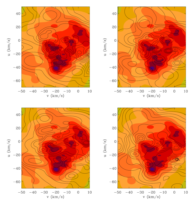
Figure 3: Overlay of simulated velocity distributions, (when the bar alone perturbs a warm exponential disk), on the observed local velocity distribution, (shown by filled contours). The radial (in units of $R_{\rm CR}$) and azimuthal coordinates of the observer corresponding to the different panels starting from the top left, are (1.8625, 25^∘), (1.9025, 15^∘), (1.9625, 35^∘) and (2.0875, 25^∘). The distributions were smoothed using the adaptive kernel method discussed in Skuljan, Hearnshaw $\&$ Cottrell (1999). Logarithmic contours have been used with inwardly increasing shading in the observed distribution. $U$ is positive along the Galactic centre while $V$ is positive along the sense of Galactic rotation. The ratio of the maximum field due to the bar at OLR to that due to the background disk is about 3.6$\%$.

3.3 Goodness of Fit

The comparison between $f_{o}$ and $f_{s}$ could perhaps be carried out visually, in terms of the degree of overlap between the $U-V$ coordinates of the 5 moving groups that are marked in Figure 2, within the error bars given by the solar peculiar velocities. However, this is hardly satisfactory; there is no direct means of quantifying this “degree of overlap”. Moreover, given the radial and azimuthal ranges that we span in our runs, and the widths of each $R$ and $\phi$ cell, each simulation generates 24$\times$9 model distributions in all the $R-\phi$ cells. Undertaking a visual comparison of each of these 216 $U-V$ distributions to the observed one, is firstly tedious and secondly subjective.

An alternative approach might be to carry out a test in order to ascertain if $f_{o}$ and an $f_{s}$ are independent. The Kolmogorov-Smirnov analysis is a typical example of such a statistical test that can check for independence of distributions. However, our distributions are bivariate $-$ this hinders the implementation of the Kolmogorov-Smirnoff scheme since it is far from robust for distributions more complicated than univariate ones. Additionally, our distributions are highly non-linear in the sense that there are parts of the $U-V$ space that are much more densely populated than others. This renders the task of judging independence of the two distributions even more troublesome.

Such logistical obstacles motivated us to adopt the less elegant frequentists’ view: we formulated a goodness of fit test that would test the (null) hypothesis H(0) that: the observed $U-V$ data is drawn from the model distribution. The conclusion is based on the $p$-value of a test statistic.

The $p$-value of a statistic is such that if it is smaller than or equal to the pre-set significance level of a test (usually taken as 0.05), then the null hypothesis is rejected at that level. Here, the significance level is the maximum probability that the statistic would be as observed, assuming H(0) to be true.

We now discuss the method of estimating the $p$-value for a test statistic S which is a decreasing measure of the goodness of fit, i.e. the better the fit, smaller is S. The reciprocal of the likelihood serves the purpose in this regard, as suggested in Saha (1998). We define the likelihood of a data set $D$, given a model distribution ($f_{M}$) at the physical location $R-\phi$ , as:

$${\bf prob}(D|f_{M})=\prod\nu_{R,\phi}(U_{i},V_{j}),$$ (2)

where $\nu_{R,\phi}(U_{i},V_{j})$ is the value of the velocity distribution function at the location ($R$, $\phi$), in the $(i,j)^{th}$ $U-V$ bin and the product is performed over all the $U$ and $V$ velocity bins.

Let $n$ (where $n$ is a natural number), data sets be drawn from a model distribution. Let the test statistic defined on one such data set be the reciprocal of the likelihood (S), such that for the $i^{th}$ of the $n$ data sets it is S_i. For the observed data set, let the statistic be (S_o). Then, we try to compute the fraction of the $n$ data sets that fit less well than the observed data, i.e. we monitor that for how many $i$, the following inequality holds:

$${\cal{\bf S}}_{i}\displaystyle{>}{\cal{\bf S}}_{o}$$ (3)

If this is true for $m$ cases, then the $p$-value for the statistic S is $m/n$. Thus, if 96$\%$ of the $n$ model data sets fit better than the real data, then the $p$-value is 4$\%$; the model is then rejected at 5$\%$ significance. In general, low $p$-values imply that the null hypothesis is unlikely to be true.

We identify a simulated distribution to be “good” if leads to the maximum possible $p$-value (of 100$\%$); the $R-\phi$ location at which this $f_{s}$ is recovered is then a “good” location. A distribution of $p$-values at each of the considered physical locations is plotted on the $R-\phi$ plane; the estimate of the $p$-value in any $R-\phi$ cell is shown as proportional to the darkness of the shading used in that cell. The darkest cells are then used to generate the $\pm$1-$\sigma$ ranges in $R$ and $\phi$ of the “good” locations. (The distribution of these “good” locations is marginalised over $\phi$ to predict the range in solar radius while the same, when marginalised over $R$, gives us the range on the bar angle.)

We also check for the scatter in the distribution of the “good” locations in the $R-\phi$ plane, obtained for any model, to confirm if the exercise undertaken here is a viable way of constraining solar position.

Even though the $p$-value is subject to a number of criticisms that can be taken into account by adopting Bayesian techniques,  it suffices to implement it in this case, since we compare the $p$-values of discrete velocity distributions that are binned into the same small number of velocity bins.

3.3.1 Comparison Between Models

Now it is to be stressed that this method of securing constrains on the “good” locations, applies for a given model, i.e. a given perturber added on a pre-fixed disc. This method also potentially allows us to seek superiority of one model over another - if the $p$-value at the location ($R_{i}$, $\phi_{j}$) in one model is less than that in another, then we can say that the address ($R_{i}$, $\phi_{j}$) is more akin to the solar position according to the former model than in the latter. In this way, we can reject one model in preference to another, only if the $p$-value in the former model exceeds that in the latter, for all $i$ and $j$. Alternatively, if the distribution of $p$-values over all $R$ and $\phi$ in one model is similar in shape to that in another model, and the $p$-value from the former model at ($R_{i}$, $\phi_{j}$), exceeds that from the latter for most $i$ and $j$, we consider the former model better than the latter. (This is why we reject Model 5 with respect to Model 4; see below).

When the differences in $p$-values alone cannot discern the viability of a model, we resort to independent dynamical considerations, in order to establish the same. The models can also be pitted against one another by checking if the right $\sigma_{U}$, $\sigma_{V}$ and $l_{v}$ have been recovered at the solar radius.

3.4 Recording the Orbits

In all our distribution diagrams, radial velocity ($U$) as observed from the Sun is positive towards the Galactic centre while transverse velocity ($V$) observed from the Sun is positive in the sense of Galactic rotation.

Usually, the orbits are recorded in the frame that rotates with the perturber. Now, the phase of the bar potential is not a function of radius, unlike the potential of the spiral pattern. Thus, the frame that the orbits are recorded in the spiral-only simulations will be static with the spiral at a certain radius but not at any other radius.

In the bar and spiral simulations the orbits have been recorded in the rotating frame of the bar. In this frame the spiral pattern is not static. Therefore we had to choose time points when the orbits could be recorded. We chose to record the orbits at those time points, when at the location of the corotation due to the bar, the potential of the spiral pattern is maximised, in the frame rotating with the bar.

It needs to be emphasised that the $f_{s}$ that we recover are not snapshots in time but are rather averages over time. This picture is therefore concordant with $f_{o}$, which presents an average over ages.

3.5 Effect of Pattern Speed of the Spiral

We want to be able to understand the structures that develop in velocity space in our bar and spiral models, as a function of the spiral pattern speed. In order to accomplish this, we invoke the important result that has been represented in Figure 14 in Paper I: stars are depleted from around the $ILR_{s}$ and pushed outwards to higher radii.

When the ratio of pattern speeds of the spiral and the bar is 25/55, $ILR_{s}$ is at $R$=1.42$R_{\rm CR}$, which is well inside the radial range being studied, ($R$=1.7$R_{\rm CR}$ to 2.3$R_{\rm CR}$). Now stars are driven away from $ILR_{s}$ to higher radii. Thus in this case, even near the inner edge of this annulus ($R$=1.7$R_{\rm CR}$), there are enough stars on prograde orbits, to contribute to the formation of relevant structures at large (negative) values of $V$, particularly the Hercules stream.

When the ILR is in the middle of the annulus under examination, (ratio of pattern speeds is 18:55) stars are depleted from around the resonance location ($R$=1.97$R_{\rm CR}$) and pushed outwards. It is shown by our bar and spiral simulations that the average number of stars just inside $ILR_{s}$ is less than in the initial equilibrium disk by about $20\%$. Thus, in this case we can expect the $f_{s}$ to suggest the observed bimodality only beyond this $ILR_{s}$. In accordance to this, we do not expect satisfactory overlap between $f_{o}$ and $f_{s}$ inside $ILR_{s}$. That is indeed what we find in our distributions. The smallest radius, at which an acceptable overlap occurs is $R/R_{\rm CR}=1.9625$.

If the pattern speed of the spiral arms is chosen so that $ILR_{s}$ almost coincides with $OLR_{b}$, (i.e. at $R/R_{\rm CR}\approx 1.7$) then the spiral is responsible for pushing stars into the annulus under investigation, from a radial location that is almost sitting at the inner edge of this annulus. However, the number of stars entering this annulus from lower radii is not as large as when the ILR lies inside the considered radial band (fastest spiral).

4 Results

The results from the different simulations are presented in this section.

4.1 Bar Only: Model 1

In this section, we present the simulations performed by perturbing the warm quasi-exponential disk with a bar, which contributes a gravitational field that is at most $3.6\%$ of the field due to the disk, at $OLR_{b}$. The $U-V$ distributions recovered at some locations have been presented in Figure 3. These are as viewed by an observer at a radial location outside $OLR_{b}$ ($R_{\rm OLR}/R_{\rm CR}\approx 1.7$), and at low azimuthal separations from the major axis of the bar; these are examples of some “good” model distributions that we spotted from those generated at different locations, at the end of the run.

One example of a model distribution that is not “good” is presented in Figure reffig:bad; this $U-V$ distribution is one that would appear to the observer who is along the bar major axis and a radius of 1.8325$R_{\rm CR}$. As is evident from this figure, the bimodality in the observed local velocity distribution is not reproduced in this simulated distribution.

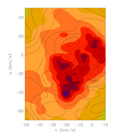
Figure 4: As in Figure 3, except that in this case, the observer location is (1.8325$R_{\rm CR}$, 0^∘). At this location, the Hercules stream is not well reproduced by the modelled velocity distribution.

The goodness of fit of the velocity distribution recovered in any $R-\phi$ cell is represented by the $p$-value of S (the reciprocal of the likelihood for the observed data to have been drawn from the model distribution) in this cell. A contour plot of the $p$-value of this statistic over the $R-\phi$ grid that we use, is presented in Figure 5.

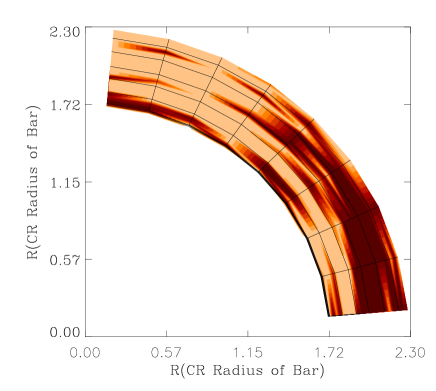
Figure 5: The distribution of $p$-value of the statistic S, (see text), as recovered from the bar-only simulation is represented as a contour plot over the relevant radial and azimuthal ranges considered. The darkness in the shading increases proportionally with $p$-value. Only the darkest $R-\phi$ cells (corresponding to $p$-value=100$\%$) are used to constrain the solar position.

From Figure 5, we can see that in general, the velocity distributions constructed at the lower azimuths comply with the real $U-V$ data. In fact, by tracking the cells at which the fit is the best, we can extract constraints on the bar parameters.

Thus, we find that analysis of the spatial distribution of the “good” models suggests that the best radial location for reproducing the observed velocity distribution is given by 2.0875$R_{\rm CR}$, with $\pm$1-$\sigma$ errors spanning the range from 1.9625$R_{\rm CR}$ to 2.1975$R_{\rm CR}$. These estimates are obtained by calculating the cumulative total of the number of azimuthal locations at a given radius, for which the $p$-value has attained its maximum. Figure 6 represents the cumulative total of the obliging number of $\phi$-locations, over the considered radial range.

Figure 6: The cumulative total of the number of azimuthal bins (expressed as a percentage of the total) at a given $R$, at which the $p$-value of the statistic S is maximum, plotted as a function of radius. The median is identified at 2.0875$R_{\rm CR}$ (solid lines), while $5/6^{th}$ ($\approx$1-$\sigma$) of the net total is achieved at $R$=2.1975$R_{\rm CR}$ (dashed lines) and the $1/6^{th}$ mark occurs at $R$= 1.9625$R_{\rm CR}$ (dotted lines). The simulation in question is the bar only simulation.

When a similar construction is sought over the azimuthal range in consideration, the result is shown in Figure 7. This figure represents the run of the cumulative total of the number of radial locations that bear the highest $p$-value, at a given $\phi$. The best azimuthal location is noted to be about 22^∘ while the +1$\sigma$ mark occurs at about 49^∘. It is hard to gauge the azimuthal location corresponding to the -1$\sigma$ error since this occurs inner to the obtained distribution.

Figure 7: As in Figure 6, except that in this case, the cumulative total of the number of radial locations (expressed as a percentage of the total), at a given $\phi$, at which the $p$-value of the statistic S is maximum, is plotted as a function of azimuth. The median is identified at about 22^∘, while $5/6^{th}$ ($\approx$1-$\sigma$) of the net total is achieved at $\phi$=49^∘. All we can say about the $1/6^{th}$ mark is that it occurs between 0 and 5^∘.

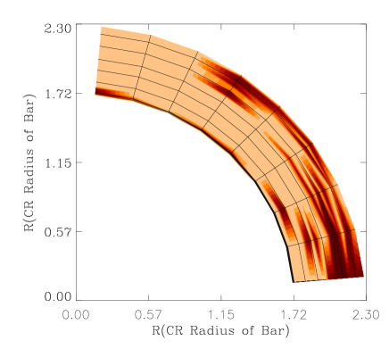
Figure 8: As in Fig 5, except that in this case, a bar and a spiral pattern together disturb the disk. The ratio of the pattern speed of the bar to that of the spiral is chosen to be 55:18 which places the $ILR_{s}$ at a radius of about 1.97 on a scale in which the $OLR_{b}$ is at 1.7 approximately.

The limits that the occurrence of the “good” models impose on the radial and azimuthal locations of the observer, can be translated to impose constraints on the bar parameters.

• The observer at the Sun needs to be separated from the major-axis of the bar by an angle which lies in the 1-$\sigma$ range of [0^∘, 49^∘], with the median of the distribution at about 22^∘.

• The observer at the Sun needs to be constrained to the radial range [1.9625, 2.1975]$R_{\rm CR}$ in our scale-free disk. If the solar radius corresponds to the median of this distribution, then $R_{\odot}=2.0875^{+0.11}_{0.125}$. Here all radii are in units of $R_{\rm CR}$. To relate these lengths to real units, let us consider the solar radius to be $8.0$kpc. This scales $R_{\rm OLR}$ to $6.51^{+0.42}_{-0.32}$kpc and the corotation radius to $3.83^{+0.25}_{-0.19}$kpc.

The constraint on the corotation radius can be translated to one on the bar pattern speed. As discussed in Paper I, the pattern speed of the bar is set to unity in our analysis, (this is what renders the corotation radius unity). Using the value of corotation radius deduced above, and the value of $220$ km s^-1  for the circular speed at the Sun, the bar pattern speed is found to be about $57.4^{+3.0}_{-2.5}$ km s^-1 kpc^-1, in the Mestel potential of our quasi-exponential disk.

4.2 Bar and Spiral Pattern

A second set of simulations involved simultaneous stirring of the warm, quasi-exponential disk by the bar and the spiral pattern.

The two different kinds of perturbers are responsible for the presence of a relatively greater variety of families of stellar orbits in these simulations. Intersection of the different generic orbits can cause local density enhancements in the velocity space; this is manifest in the numerous small clumps visible in the central parts of the velocity distributions at many locations. However, the overall form of the velocity distributions approaches the observed $U-V$ diagram; this is also borne by the distribution of $p$-value of the statistic S over the first quadrant of the outer part of the disc that we study (Figure 11).

4.2.1 Lowest Ratio of Pattern Speeds: Model 2

In Figure 8, we present the distribution of $p$-value of S, obtained by perturbing the warm quasi-exponential disk by a bar and a spiral pattern simultaneously. The maximum gravitational field due to the perturbation is about $4.9\%$ of that due to the background potential. The ratio of the pattern speeds is $\Omega_{\rm sp}:\Omega_{\rm bar}$=18:55.

From the distribution of $p$-value in this case (Figure 8), we can extract the locations where the model velocity diagrams fit the observed one the best (i.e. where $p$ is highest). An analysis of such “best” locations is carried out along the lines of the analysis discussed in the previous section. This yields the following constraints from this simulation:

• The distribution of the highest $p$-value over radii, has its median at $R$=2.0925$R_{\rm CR}$, with the +1-$\sigma$ and -1-$\sigma$ at $R$=2.21$R_{\rm CR}$ and $R$=1.95$R_{\rm CR}$, respectively. Placing the Sun at the median of the distribution of the best model locations with radius, we get the bar pattern speed to be 57.5${}^{+3.2}_{-2.9}$ km s^-1 kpc^-1.

• The distribution of the highest $p$-value over azimuth, has its median at $\phi$=15^∘, with the +1-$\sigma$ and -1-$\sigma$ at $\phi$=30^∘ and $\phi\in$[0,5]^∘ respectively.

Thus, it appears that the “best” values of bar angles that this simulation predicts is similar in range to that predicted by the bar-only simulation. However, the radial range corresponding to the “good” models, is slightly skewed towards higher radii in this case than in the other in the sense that higher radii are found compatible with the solar position, in this case. This too is only to be expected for the chosen pattern speed of the spiral which places the ILR at about $R$=1.97$R_{\rm CR}$, thus causing depletion of stars from around this radius, at the expense of enhancing the number of stars at higher radii (see Section 3.5).

4.2.2 Highest Ratio of Pattern Speeds: Model 3

In these simulations, the ratio between the spiral and the bar is maintained at 25/55. This places $ILR_{s}$ well inside $OLR_{b}$. The ratio of the perturbative and background fields is about $0.049$ at the $OLR_{b}$. The distribution of the $p$-value of S is shown in Figure 9. From Figure 9, we learn that:

• the observer has to be constrained to radii between $R/R_{\rm CR}$= 2.0875${}^{0.15}_{0.25}$, in order to suggest satisfactory overlap between the model and observed distributions. Here the errors are 1-$\sigma$ errors as usual. This implies that the bar pattern speed is 57.4${}^{4.1}_{6.9}$ km s^-1 kpc^-1.

• The best value of the bar angle is 6^∘, though this value can vary within the 1-$\sigma$ range of [0^∘, 43^∘].

The bimodality observed in the local velocity distribution comes out clearly in the distributions recovered from this simulation (Figure 10). The other moving groups marked in the local velocity distribution, are also reproduced.

4.2.3 Intermediate Ratio of Pattern Speeds: Model 4

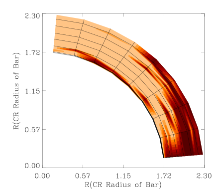
Figure 9: Similar to Figure 8 except that the pattern speeds of the spiral arms and the bar are in a ratio of $25:55$.

The ratio of pattern speeds between the spiral pattern and bar is chosen to be 21/55 in this simulation. This places $ILR_{s}$ almost on top of $OLR_{b}$. The two perturbers together produce a gravitational field that is at most $4.9\%$ of that due to the background disk. Figure 11 shows the bivariate distribution of $p$-value of the test statistic S.

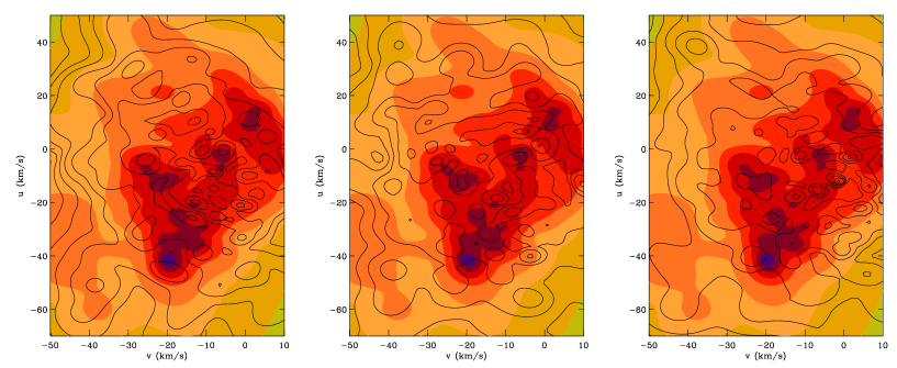
Figure 10: Similar to Figure 3 except that in this case, a spiral pattern disturbs the disc along with the bar; the pattern speeds of the spiral arms and the bar are in a ratio of $25:55$. The observer locations for the above distributions are (1.9625, 35^∘), (2.0125, 25^∘) and (2.1125, 25^∘) starting from the top left-hand panel.

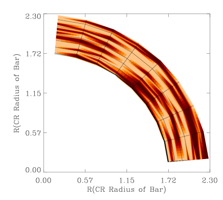
Figure 11: Similar to Figure 8 except that in this case, $ILR_{s}$ occurs almost at the same physical radius as $OLR_{b}$.

As is evident from Figure 11, this distribution is rather different from the distribution shown in Figures 9, 8 and 5. The essential difference lies in the fact that in this case, the regions corresponding to the highest $p$-value are strewn all over the range of the $R-\phi$ space that we record the orbits in. In the previous runs, the distribution of the locations corresponding to the best models was much less non-linear. In fact, this $p$-value distribution bears a strong resemblance to that which results from a spiral-only simulation, (see below).

Since the “good” locations are too scattered in the $R-\phi$ plane,

it is, rather meaningless to try and use this simulation to extract the relevant bar parameters.

4.3 Spiral Only: Model 5

Model velocity distributions were also obtained from simulations in which the 4-armed spiral pattern alone perturbed the warm quasi-exponential disk. The results discussed below pertain to spiral-only simulations that were performed with all of the three used pattern speeds.

The distributions obtained in this simulation, are characterised by structures that stand out less boldly than those observed when the bar is a perturber though the number of velocity space structures is much more in this case. Now, the potential of the logarithmic spiral has a radial dependence. At a given azimuth, stars on varying radii are at different relative phases compared to the maxima in the potential well of the spiral pattern. Thus, the cumulative effect at this azimuth is in general due to the superposition of orbits with different orientations. (At a given azimuth and at two close radii, orbits will in general differ only slightly in orientation unless the radii under consideration straddle a principal resonance location). Such superposition of orbits can lead to local density enhancements in velocity space. This would render the velocity distributions inundated with structures on small length-scales in the $U-V$ plane.

In order to check if this formed structure is compatible with the same in the observed distributions, we check the distributions of our goodness-of-fit statistic (Figures 12).

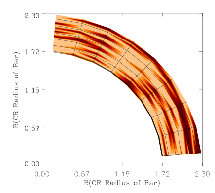
Figure 12: Similar to Figure 8 except that in this case, a spiral pattern perturbs the disk alone. The pattern speed of the perturber is 18/55 times that of the bar and the used spiral contributes a gravitational field that is at most 3.6$\%$ of that due to the background disk, at $OLR_{b}$.

From the distribution of the $p$-value in this simulation, we notice the following:

• There is a dearth of continuous bands of “good” locations; instead, the $R-\phi$ cells corresponding to the “good” models, are strewn all over the band under consideration. This is unlike the results obtained from simulations done with the bar alone and the bar and spiral simulations in which the slowest and fastest spirals have been used (Figures 9, 8 and 5). The result presented in Figure 12 bears similarity to that obtained from the simulation done with the bar and the spiral pattern of intermediate speed (Figures 11). An attempt will be made in Section 6.1, to understand the origin of this clumpy nature of the distribution.

• The spiral alone is found to cause insufficient disk heating. Using a higher perturbation strength does not improve the situation much. This will be talked about in Section 6.

• The highest $p$-value is lower in this case compared to when the bar is included.

Given the highly non-linear form of the distribution of the maximum $p$-value in this simulation, we will not resort to constraining the solar position from this simulation. (The recovery of the bar angle from this spiral-only run is of course not valid).

4.4 Dispersions

It is important to check that the velocity dispersions of the configuration at the end of a run, at a radius that can be identified with the solar position, is compatible with that estimated in the solar neighbourhood from observations. Needless to say, dispersions vary with the choice of the stellar samples. However, the sample of initial conditions that we numerically integrate is not distinguished by differences in age or metalicity. Also, the $f_{o}$ that we compare our $f_{s}$, is constructed from $all$ the single stars that obey certain cutoffs in the Hipparcos Catalogue. Thus, our recovered values of dispersions will be averages over all ages. All we hope for is that the runs result in dispersions that lie within the ranges pertinent to an average sample in the solar neighbourhood: from main sequence stars to giants. This is indeed found to be the case, as apparent from a comparison of the values of $\sigma_{U}$, $\sigma_{V}$ and $l_{v}$ shown in Figure 13 from the different models, with Table 10.2 and Table 10.3 of Binney $\&$ Merrifield (1998) (pages 632-633). It is to be noted that the presented quantities are azimuth averaged, at the medial value estimated for the radius of the Sun, from the corresponding run. When it is not possible to extract the solar position from a simulation, the radius is chosen to be equal to that obtained from the bar-only simulation.

It may be noted that while the vertex deviation at the solar radius is acceptable for all the models, for the spiral-only run, the Oort ratio ($\sigma_{V}^{2}$:$\sigma_{U}^{2}$) is almost as low as the lower limit for the old stellar disk (of about 0.42) from Hipparcos (Dehnen $\&$ Binney 1998). This is most probably an offshoot of the weakness of the spirals that we work with, as explained in Section 2.

Figure 13: Left panel shows plots of azimuth averaged radial (filled circles) and tangential velocity dispersions (open circles), as obtained at the recovered solar radius, at the end of the simulation, for each of the five different runs that were conducted. These are as follows: (1) bar-only (2) bar and fastest of the three spiral patterns (3) bar and slowest of the spirals (4) bar and spiral when the ILR of the spiral concurs with the physical location of the OLR of the bar (5) spiral-only. Models 4 and 5 do not allow a solar position to be extracted; in these cases, the dispersions were extracted at an $R$ that was identified as the solar radius in the bar-only simulation. The azimuth averaged vertex deviation at the solar radius is shown in the right panel.

Table 1: Table showing the results obtained from the five different runs that have been presented in this paper. The third, fourth and fifth columns respectively depict the value of the azimuth averaged $\sigma_{U}$ and $\sigma_{V}$ and $l_{v}$, at the end of the run, at a radial location that is identified as the median of the 1-$\sigma$ range of radii that are found compatible with the solar radius. The next two columns refer to the value of the bar pattern speed and angle, as inferred from the relevant run. Models 4 and 5 imply highly scattered distributions of the locations where the observed velocity diagram is well reproduced (see text). These models therefore fail to provide adequate constraints on the solar position and hence cannot be used to extract the bar parameters.

 

Number Model $\sigma_{u}$ (kms^-1) $\sigma_{v}$ (kms^-1) $l_{v}$ (degrees) $\Omega_{\rm bar}$ (kms^-1kpc^-1) Bar Angle (degrees) 1 bar-only 35.51 18.96 20.1 57.4${}^{+3.0}_{-2.5}$ 22${}^{+27}_{-22}$ 2 bar $\&$ spiral, $\Omega_{\rm sp}$ = 25/55$\Omega_{\rm bar}$ 35.75 19.67 20.6 57.4${}^{+4.1}_{-6.9}$ 6${}^{+37}_{-6}$ 3 bar $\&$ spiral, $\Omega_{\rm sp}$ = 18/55$\Omega_{\rm bar}$ 34.18 19.84 21.0 57.5${}^{+3.2}_{-2.9}$ 15${}^{+15}_{-15}$ 4 only spiral, $\Omega_{\rm sp}$ = 25/55$\Omega_{\rm bar}$ 33.40 19.74 22.6 $--$ $--$ 5 bar $\&$ spiral, $\Omega_{\rm sp}$ = 21/55$\Omega_{\rm bar}$ 30.37 19.45 21.2 $--$ $--$

 

5 Orbits

It is expected that just outside the $OLR_{b}$, stars are on orbits which are aligned with the major-axis of the bar while just inside, anti-aligned orbits prevail. The radial location of the Sun, it is also expected to be visited by stars which are scattered off the Outer $1:1$ Resonance, (the $-1:1$ resonance). This resonance is defined by the following rule.

$$-1=\frac{\kappa}{\Omega-\Omega_{\rm p}}$$ (4)

Here $\kappa$ and $\Omega$ are the epicyclic and azimuthal frequencies while $\Omega_{\rm p}$ is the pattern speed of the perturbation. Eqn. 4 implies that this resonance occurs at a radius of about $2.41$ in units of the corotation radius. It is possible that stars can reach the solar circle from the vicinity of this resonance. Thus, near the Sun, we can expect orbits belonging to the the x₁(1) family, (orbits aligned to the bar), the x₁(2) family at negative $U$ and $V$ velocities, (anti-aligned orbits) and the $-1:1$ type orbits. We also expect a plethora of chaotic orbits, especially around the location of the OLR. The nomenclature used here is that of Contopoulos $\&$ Grosbol (1989).

5.1 Stars on “hot” orbits

The orbit in the left panel of Figure 14 is due to a star at position coordinates $R/R_{\rm CR}=2.04$ and azimuth 35^∘), at very large negative radial and tangential velocities, ($U=-81$ km s^-1, $V=-40$ km s^-1). The velocities characterising this orbit are high enough to place this star well outside the Hercules stream, (towards more negative radial velocities), in the $U-V$ plane. This orbit can be ruled out as chaotic on the basis of the smooth surface of section (right panel in Figure 14. This orbit is noted to librate around a closed aligned orbit.

Figure 14: Figure showing orbit (left panel) and its surface of section (right panel), of a star with initial velocities $U=-81$ km s^-1, $V=-40$ km s^-1, near the solar radius. This orbit is parented by a closed aligned orbit. The circular orbit at this radial location is marked by crosses. The bar is static in this frame that rotates with it. The major axis of the bar is shown by the solid horizontal line. This orbit corresponds to an energy in the rotating frame of the bar, that just exceeds the range of energies that characterise orbits that are susceptible to cross the corotation and escape to much larger radii. We observed such orbits only at radial velocities less than -70 km s^-1  in the $U-V$ plane; such a constraint on $U$ suggests that only regions outside the Hercules stream, (as marked in Figure 2) are due to these “hot” orbits. The bar is strong enough to contribute a gravitational field at the OLR that is at most $3.6\%$ of the field due to the background potential.

The parent of this orbit could have originated just outside the OLR. It is also possible in principle, that the birthplace of the closed aligned orbit was inside corotation; at a radius just inside corotation, stars are sired primarily by closed aligned orbits. A star can foray to the solar radius from such radii, only if it is highly energetic. The orbit presented in Figure 14 is indeed characterised by a very high energy. Thus it is possible that this is one of the “hot” orbits which Raboud et. al (1998) and Fux (2000) claim to be the building blocks of the Hercules stream. To ascertain the birth place of the star which is on the orbit in Figure 14, we decided to examine its energy. In the rotating frame of the bar, the Jacobi integral ($J$) provides the value of the Hamiltonian.

$$J=\frac{U^{2}}{2}+\frac{(V+v_{0}-|{{\bf R}\times{\bf\Omega_{\rm p}}}|)^{2}}{2}+\Phi_{\rm eff}$$ (5)

Here $U$ and $V$ are velocities recorded, with respect to the Sun, $v_{0}$ is the amplitude of the uniform rotation curve and $\Phi_{\rm eff}$ is the effective potential, given by:

$$\Phi_{\rm eff}=\epsilon_{0}\frac{\cos(2\phi)}{R^{3}}+\ln{(R})-\frac{\Omega_{\rm p}^{2}}{2}R^{2}$$ (6)

where, $\epsilon_{0}$ is the maximum strength of the bar ($=0.06$) and $\phi$ is the azimuth. It may be noted that in Eqn 5, the solar peculiar velocities have been ignored. If the value of the Jacobi integral exceeds the effective potential at the unstable Lagrange points, a star inside corotation is in principle able to escape to infinity. It is the Coriolis term in the equation of motion (written in the rotating frame), that in general prevents the star from doing so. But even so, such stars can easily visit the solar neighbourhood, from a location inside corotation. Fux (2000) and Raboud et. al (1998) call such stars to be on “hot” orbits.

To check if the orbit shown in Figure 14 is “hot”, we first identified the Lagrange points for the effective potential defined in Equation 6. The value of the Hamiltonian for a star on this orbit was then calculated and compared against the value of $\Phi_{\rm eff}$ at the saddle points of this potential structure. We found that this orbit is just energetic enough to be termed “hot”; the Jacobi integral characterising this orbit exceeds the effective potential at the saddle points (which are also the unstable Lagrange points) by about $0.123\times{10^{3}}{\rm km}^{2}{\rm s}^{-2}$.

A neighbouring orbit ($U$=-81/kms and $V$=-43/kms) is definitely hot. It is shown in Figure 15. The surface of section of this orbit manifests its chaotic nature. The Jacobi integral exceeds the effective potential at the saddle points in $\Phi_{\rm eff}$ by $1.08\times{10^{3}}{\rm km}^{2}{\rm s}^{-2}$.

Figure 15: Similar to Figure 14. This is the orbit charted out by a star with velocities $U=-81$ km s^-1, $V=-43$ km s^-1, near the solar radius. The orbit is definitely irregular as implied by its surface of section; no smooth curve was found to join the occupied islands of phase space. Considerations of the Hamiltonian of this orbit suggested that this is a “hot” orbit.

Thus, our conclusion is that the progenitor of the orbit in Figures 14 and 15 lie inside corotation radius in the initial equilibrium disk and stars on these orbits are pushed to much larger radial locations, owing to their energies in the frame of the bar.

However the “hot” orbits cannot be considered responsible for the Hercules stream since they lie substantially outside the Hercules stream on the $U-V$ plane. On the other hand, such a conclusion is subject to the definition of the exact boundaries of the Hercules stream. It is rather difficult to search for exact confinement of individual moving groups in the local velocity space. According to the local velocity distribution diagram presented in Dehnen (2000), the star on this “hot” orbit would indeed lie within the region of velocity space that is dominated by late-type stars. Dehnen refers to this mode of the local velocity distribution as the “OLR” mode; his OLR mode is the analogue of Fux’s Hercules stream. Differences between the methods used by Dehnen and Fux in the construction of the velocity distribution function and the considered stellar samples, were responsible for variation in the details of the respective distribution diagrams. Thus Dehnen’s OLR mode covers greater area in the $U-V$ plane than Fux’s Hercules stream.

In light of the above discussion, it appears that the following will be safe to conclude: we spotted stars at very high radial velocities which were found to be on “hot” orbits, and did not find any stars on such orbits at $U\leq 70$ km s^-1. The moderate to highly “hot” orbits were found to be chaotic.

5.2 Hercules stream

A number of stars in the Hercules group were observed to be on quasi-periodic orbits belonging to the anti-aligned family though it appears that this stream is composed of chaotic orbits too. We found a plethora of chaotic orbits in this group - the closer the observer is to the principal resonance due to the bar, the greater is the fraction of such chaotic orbits.

5.3 Hyades-Pleiades stream

It appears that the less energetic stars in this group are due to the outer $1:1$ resonance. In addition to the $-1:1$ family, there are also orbits of the aligned family. By constructing surfaces of sections for stars in this part of the $U-V$ plane, we have realised that in addition to these orbits, there are also a number of highly irregular orbits that constitute the Hyades-Pleiades group.

Of course, once the spiral arms are introduced along with the bar, the families mentioned above interact with the orbits generic to the region around $ILR_{s}$. As is borne by the distributions presented in Section 4.2, this affects the velocity space by introducing local density enhancements and washing out prominent clumps. The structure of phase space in this case is better understood in light of a brief orbital analysis when the spiral wave is the sole perturber. This is dealt with in the following section.

6 Discussion

This section is devoted to detailed discussion of the results presented above.

6.1 Origin of the Scatter in the $p$-Value Distribution

As we have seen above, the spatial distribution of the $p$-value of S is marked by a high degree of scatter, for the spiral-only simulations and the run in which the major resonances of the two perturbers coincide. For the other simulations, the locations corresponding to the “good” models are less spread out over the quadrant of the radial band that we study. In this section, we question the origin of this behaviour.

It is envisaged that such a trend can be addressed only in terms of the orbits that characterise the model velocity distributions. We investigate the orbits in different $R-\phi$ cells, for the spiral-only simulation in details. This simulation is preferred over the special bar and spiral simulation mentioned above, since it is relatively easy to interpret the results when there is a single perturbation instead of two. Besides, given that we are dealing with a 4-armed, tightly wound spiral pattern, the effect is nearly axisymmetric; therefore, we expect the azimuthal dependence of the velocity distributions (at a given $R$), to be relatively less in the spiral-only case.

We note the following trends in our results:

• Trend 1-
  A direct anti-correlation is found to exist between $p$-value of the statistic and the evenness in the distribution of the loop orbits between the apocentric and pericentric radii. Thus, when the orbit fills out the annulus between these two radii almost uniformly (left panel in Figure 16), $p$-value is lower than when the orbits falls on itself consistently, i.e. the same path is repeated in configuration space (right panel in Figure 16).

• Trend 2-
  At any radius, the azimuth-averaged $p$-value of S is found to roughly vary periodically with $R$. This is shown in Figure 17.

• Trend 3-
  The overall distribution of the $p$-value is not affected by the pattern speed of the spiral used in the spiral-only simulation; the strength of the clumps in this distribution may vary slightly with the position of $ILR_{s}$.

• Trend 4-
  Beyond $R\approx$1.8$R_{\rm CR}$, the distribution of the “good” models in the spiral-only case look very much like that in the bar and spiral simulation, when the two resonances concur. In addition to the approximate radial periodicity in the occurrence of the “good” models, the distributions of the $p$-value are noted to be highly scattered in both Models 4 and 5.

Figure 16: Orbits in the presence of the perturbation due to the spiral alone, at an azimuth of 35$\circ$ and radii of 1.8625 (left panel) and 1.9375 (right), on a scale in which the ILR of this spiral pattern occurs at a radius of 1.42 approximately. Both are stable orbits.

Figure 17: Azimuth averaged $p$-value of S, plotted as a function of radius for the case of the spiral-only simulation (solid lines) and the resonance overlap case (broken lines). In both cases, the variation in the $p$-value is noted to be similar except that its amplitude is higher in the case when the resonances coincide.

Now we attempt to qualitatively understand the 4 trends itemised in the last paragraph.

• Understanding Trend 1-
  It is quite straightforward to realise why the even-ness of distribution of the orbit within the pericentre and apocentre should be strongly anti-correlated with the $p$-value. When the orbit is as in the left panel in Figure 16, the resultant of the velocity vectors, taken over varying phases, implies a radial velocity that is clustered strongly around zero and $V$ clumped preferentially at a high positive value, if the sense of motion along the orbit is positive, otherwise the peak of $V$ is strongly negative. In general, this picture will not correspond to the definite structures that are observed at distinct locations on the $U-V$ plane, in the solar neighbourhood.

• Understanding Trend 2-
  However, the main question is why the orbit folds upon itself at certain radii but deviates from this configuration at other radii. In fact, the variation of $p$-value with radii, in a spiral-only simulation is found to be roughly periodic, as shown in Figure 17. We need to understand the origin of this periodicity.

  Whether an orbit is going to fold upon itself or it is going to be highly excursive will be given by the initial conditions and some kind of an integral of motion, which must in turn relate to the potential. In our scale free units, the perturbing potential of the spiral is:

  $$\Psi_{sp}(R,\phi)\sim\displaystyle{\frac{\cos[4(\phi-\Omega_{\rm sp}\Delta{t})-\alpha\ln{R}]}{\sqrt{R}}}$$ (7)

  where $\Omega_{\rm sp}$ is the pattern speed of our 4-armed spiral pattern, $\Delta{t}$ is the time that has elapsed and $\alpha$ is related to the pitch angle $i$ of the spiral as $\alpha=4\>{\cot}(i)$. This implies that whatever the exact form of the relevant integral of motion is, it will be roughly periodic in $\ln{R}$.

  Thus, the volume between the pericentre and the apocentre is given by an integral of motion that is akin to the component of the angular momentum that is orthogonal to the plane of the disc ($L_{z}$). In the axisymmetric case, it is indeed given by $L_{z}$, where

  $$L_{z}^{2}=\displaystyle{\frac{1}{R^{3}}\left(\frac{\partial\Psi_{sp}}{\partial{R}}\right)}$$ (8)

  Thus, it is clear that in our spiral only simulation, the radial extent of excursion that these orbits are allowed, varies periodically with the initial radial position of the star on this orbit. This is indeed what is noted from the run. It is to be noted that the discussion above included only stable orbits.

• Understanding Trend 3-
  This explanation would hold good irrespective of $\Omega_{\rm sp}$ used.

• Understanding Trend 4-
  Regular orbits are harder to spot in the case of the spiral and bar jointly perturbing the disc, with their major resonances coinciding. In this configuration the distribution of $p$-values resembles that of the spiral-only case and it does not look like that in the other three models. The variation of the azimuth averaged $p$-value at any radius varies with radius nearly periodically, (plot in broken lines in Figure 17) while this quantity is not at all periodic with $R$ in the other cases. Why is this so?

  Qualitatively, we may try to understand this trend by querying what it is between the spiral-only and the resonance overlap cases that is common, which is but different from the other three models? Well, in these two cases, the dynamical influence of the spiral pattern is not swamped by that of the bar, unlike the other three cases. Now, the coincidence of the major resonances at $R\approx 1.7R_{\rm CR}$ is an example of resonance overlap. As Walker $\&$ Ford (1969) pointed out, when multiple resonances occur sufficiently closely, the system is not only rendered nonintegrable, but extensive chaos also sets in. This is what is predicted to happen in this case, as suggested previously by Quillen (2003). So is it possible that global chaos is triggered in the spiral-only case too but the introduction of the bar inhibits this effect? To answer this question, we need to recall what the spiral does, as distinguished from what the bar does.

  As we have mentioned before, stars are drifted outwards from $ILR_{s}$. The bar on the other hand, distorts orbital configurations with respect to its major axis. Thus, if we have an $R-\phi$ cell that is being visited by orbits of opposite orientations, then it is possible that a systematic decrement occurs in the value of one of the components of the velocity vector. In the spiral-only case though, the orbits that superpose are nearly of the same configuration; such superposition leads to an enhancement in the velocity. Thus, the kinetic energy keeps building up in the spiral only case, and in the process of this build-up, if the kinetic energy crosses a threshold, then it is possible that chaos sets in $-$ chaos that is strong enough to disrupt the orbital families that support the spiral. Once such chaos sets in, the superposition of the velocity vectors of the stars at different phases on it may coincidentally add up to produce a feature in velocity space that is akin to one of the observed streams. There is no reason to expect the “good” locations to be confined to well defined bands when this happens. This is a qualitative argument to explain the high scatter that is noted in our spiral-only runs.

6.2 Distributions

In the $U-V$ distributions that are identified as “good’, it is found that the simulations replicate the observed velocity space structures quite well. More importantly, the locations that correspond to low (lower than maximum) $p$-values for the considered statistic, bear distributions that do not visually resemble the observed local velocity distribution. This offers confidence in the usage of the $p$-value of S as an indicator of the goodness of fit.

In the “good” distributions, the bimodality is found to be clearly marked. In such $f_{s}$, as in $f_{o}$, the Hercules stream represents a smaller probability density in the velocity space than the other four streams. At lower radii, greater structure is observed than at higher radii; in particular the region of the velocity space around the moving groups, Hyades, Pleiades and Coma Berenices is heavily crowded with structure.

Other than the 5 moving groups that we focus upon in this work (namely, Hercules, Hyades, Pleiades, Coma Berenecius, Sirius), in most of the “good” distributions, we consistently notice two structures which are not currently distinguished as moving groups:

• A clump often shows up in the “good” distributions, at about $U=20$ km s^-1and $V=-20$ km s^-1.

• All the good model distributions, display a finger-like feature that extends from about $U=40$ km s^-1and $V=0$ km s^-1to about $U=50$ km s^-1and $V=-20$ km s^-1. This feature is also noted in the observed local $U-V$ diagram. Perhaps, this could be explained as a low-density moving group, such as the Hercules stream.

6.3 Relative Significance of Bar and Spiral

It is found that the bar alone can reproduce the observed velocity structures quite well, though the bar alone simulations (visually) appear to be responsible for clumps that are bolder than those spotted in the $U-V$ plane in the bar and spiral simulations, (compare Figure 3 to Figure 10). In fact, the extra wispiness which characterises the distributions from the bar+spiral simulations, seems to render the $U-V$ diagrams more close to the observed distribution. However, such a judgement is based on visual comparison and is therefore purely qualitative since our goodness of fit parameter is not able to deal with this facet of the comparison. Thus, a visual check may suggest that the bar only simulations are not sufficient to model local kinematics, but unless the goodness of fit parameter is refined to include appreciation of the sub-structure of the clumps in velocity space, it cannot confirm any such conclusion. At the moment, the comparison is made merely on the basis of the position and extent of these clumps, within error bars given by the solar peculiar velocity components.

Inclusion of the spiral arms reduces the boldness of the features that show up in $f_{s}$. We realised that the presence of the extent of fine structure in the distributions was a function of the chosen ratio of pattern speeds of the spiral wave and the bar. With the appropriate choice of $\Omega_{\rm sp}$, we can ensure that more stars enter the solar neighbourhood from lower radii when the models included the spiral pattern than when it was left out. We could use this ratio as a tool to control the prominence of the Hercules stream. Smoothening of the local phase space by even other scattering agents could further improve the overlap between the model local distributions and their observed counterpart.

Another reason why the spiral pattern is efficient in diluting the boldness of the structures is actually due to the way we choose to record the orbits. The orbits are recorded in the rotating frame of the bar, in which, the spiral pattern is obviously not static. Neither is the phase of the potential of the logarithmic spiral the same, with respect to that of the bar, at all radii; the phases of the two potentials coincide only at the corotation due to the bar. Thus, in general, within a given radial bin, superposition of orbits of slightly different phases occurs. This leads to a slight washing off of the bold features in the velocity plane, causing an increase in the wispiness of the velocity structures.

However, we can convince ourselves of the importance of including the spiral pattern in the modelling in another way. The interarm separation of the spiral pattern used in our work is about 3.4kpc, given that the pitch angle of this pattern is $15^{\circ}$, the number of arms is 4 and that the Sagittarius arm lies at about 6.5kpc (Melnik 2006; Vallee 2002). If the average epicyclic excursion of stars in the Solar neighbourhood exceeds this interarm separation, then spiral arm scattering can be ruled out as important. Now, if the epicyclic amplitude of a star with a guiding centre at $R_{\rm G}$ is $X$, then after time $t$, the star is at a radius

$$R=R_{\rm G}+X\cos{(\kappa{t})}$$ (9)

Here $\kappa$ is the epicyclic frequency which is given by $\displaystyle{\frac{\sqrt{2}}{R}}$ in the Mestel potential. We can set the average $\dot{R}$ to the radial velocity dispersion $\sigma_{\rm U}$, which is about 35 km s^-1at the solar circle, after the perturbation has steadied. Thus, taking the time derivative and then the averages of both sides of Eqn 9, we get that $X\approx\displaystyle{\frac{\sqrt{2}\sigma_{\rm U}}{\kappa}}\approx 1.25$kpc. Therefore, on the average, the total epicyclic excursion of a star in our simulations is about 2.5kpc. This is less than the inter-arm separation of the spiral pattern used in our work. Thus the scattering induced by the spiral pattern in our models cannot be ruled out. Hence any modelling that does not take such effect into account is incomplete.

6.4 Origin of the Moving Groups

The extensive set of stellar kinematical information that Hipparcos provided, has opened up the possibility of constructing velocity distribution diagrams in our neighbourhood. While workers differ in the details of this portrayal (Dehnen 1998; Fux 2000; Skuljan et. al 1999; Chereul et. al 1998), one feature that is clearly evident is a bimodality in the local velocity distribution; this can also be identified as the location of the Hercules stream in the $U-V$ plane, away from the other moving groups. As Famaey et. al (2005) indicate, there are three broad classes of mechanisms that have been invoked in this context, with the aim of describing the observed moving groups, and in particular, the emergence of this bimodality.

The most traditional of these is to correlate the moving groups with irregularities in the star formation rate. However, such a scenario fails to reconcile with the spread in age shown by stars within a moving group. Discussions about the span of ages present in any of the streams is beyond the scope of our current methodology. The inclusion of transient spirals or episodic growths in bar strength in the modelling, can help in this regard.

Another future project is envisioned in which the radial velocity and metalicity information of a very large number of nearby stars, as provided in the RAdial Velocity Experiment (RAVE) data set (Steinmetz et, al 2006), supplemented by transverse velocity data of the same stars from the Hipparcos measurements, will be implemented into an algorithm like the one we used here, in order to identify the original galactocentric locations of these stars that results in a metalicity/age distribution that is observed today. As the quality of kinematic data in the solar neighbourhood improves, we will have better constraints to check our models against.

A merger scenario, could also be invoked to explain the moving groups observed in the disk in our neighbourhood; the merger in question is between the Milky Way and a satellite galaxy. After all, this mechanism has been solicited to explain streams in the halo, near the solar position (Helmi et. al 1999) and the Arcturus group (Navarro et. al 2004). However, given that these distinct moving groups are observed in the disk, it would be (statistically speaking) improbable for them to be all merger remnants.

Alternatively, it is the dynamical influence of the bar that is sometimes called upon to explain the moving groups. As explained above, Kalnajs attributes the bimodality in the local $U-V$ diagram to orbits that have been scattered off the OLR of the bar, as recorded by an observer at the Sun, sitting near or just outside this OLR. Dehnen (2000) agrees with this while Fux (2000) suggests that the Hercules stream is made up of “hot” orbits that have been discussed in Section 5. Fux (2001) proposes that the Hercules stream is due to an overdensity of chaotic orbits; the chaos resulting from the bar achieving a major resonance in the vicinity of the solar radius. A plethora of chaotic orbits have been spotted in our bar-only simulations too.

6.4.1 Why the Hercules stream?

In the light of our results, it appears that though the Kalnajs mechanism can adequately explain the very visible bimodality in the local velocity space, it is not relevant to the splitting of the structure at the less negative tangential velocities (i.e. the velocity mode other than the Hercules stream) into the four (or more) individual moving groups. Strictly speaking, even the origin of the Hercules stream is not as clean as the Kalnajs mechanism suggests since in our bar-only simulations, we find that there is greater variety besides the anti-aligned orbits. At the same time we cannot agree that there are only “hot” orbits in the Hercules stream; in fact, the “hot” orbits manifest themselves only at $U\leq-70$ km s^-1. Thus, the hypothesis proposed by Raboud et. al (1998), Fux (2000) and Fux (2001) is not satisfactory either.

The bar used in our simulations was imposed on a warm quasi-exponential disk. An important observation that can help us to resolve the puzzle of the origin of the streams is that our simulations done with a much weaker bar on a cold Mestel disk produced a very clean and well-defined bimodality in the velocity space around the location of the OLR of the bar; one part of the $U-V$ plane is occupied by aligned orbits while the other part is due to anti-aligned orbits. For this setup, it was noted that there are very few stars that were not members of these groups of aligned and anti-aligned orbits. Also, these two groups in the velocity plane appeared coherent and not split into further sub-clumps. All this is clear from the distributions presented in Paper I.

These findings lead us to the following conclusions:

• The presence of the aligned and anti-aligned modes in the distributions obtained from the cold background model suggests that the Kalnajs mechanism is certainly effective in the formation of the Hercules stream.

• In contrast to the observed velocity distribution, the lack of splitting of either of the aligned or anti-aligned groups in the cold disk scenario suggests that as the underlying distribution of stars in the disk becomes hotter and the bar develops to higher strengths, stars will tend to get more energetic and will be less likely to be trapped in a family of a certain orbital configuration. Instead, stars in the radial regions close to the Sun will then be more susceptible to the more minor resonances, such as the -1:1 resonance that occurs outside the solar radius. This will be manifest in the high degree of structure noticeable in the $U-V$ plane.

Thus, we propose that a good way to view the situation in the solar neighbourhood is to consider it as a progression from the case of the cold disk being perturbed by a weak bar towards a configuration marked by higher perturbation strengths and increased background stellar velocity dispersions.

We should stress the fact that the cold disk simulations in question had a $1/R$ surface density profile. As the observer moved away from the OLR to higher radii, the prominence of the anti-aligned family decreased in the velocity plane. However, such an observer location will continue to be visited by stars from the inner disk, more so if the surface density profile is changed so that it is approximately exponential. Then, even at the solar circle, (which is outside the OLR of the bar) there will be more stars coming from lower radii than in a disk with a $1/R$ profile; these will contribute strongly to the Hercules stream. Thus the Kalnajs mechanism is the basis of the bimodality of the velocity distributions around a principal resonance of an $m=2$ perturbation. In the presence of parameters realistic to the solar neighbourhood, other effects show up.

6.4.2 What of Model 1?

From the distributions that we recover from our bar-only simulations, it seems that the bar alone is sufficient to explain the moving groups. However, as we have seen above (Section 6.3), the average epicyclic excursion of a star (locally) is less than the inter-arm separation of the four-armed spiral pattern typical of our Galaxy. This implies that the modelling of local kinematics is incomplete without the effects of the outer spiral pattern being taken into account. In other words, even though our goodness of fit parameter indicates otherwise, dynamical reasoning suggests that Model 1 is not satisfactory.

6.4.3 What of Model 5?

The spiral only runs lead to a value of $\sigma_{U}\approx 30$ km s^-1, $\sigma_{V}/\sigma_{U}\approx 0.66$ and $l_{v}\approx 21^{\circ}$ in the disc, at the solar radius. This combination of values is neither compatible with the counterparts of these quantities for any of the $B-V$ colour bins into which (Dehnen $\&$ Binney 1998) divide the Hipparcos sample of main sequence stars nor with the same for the non-main sequence stars the kinematic information of which is given in Table 10.3 in Binney $\&$ Merrifield (1998). However, it is always possible that these quantities that we recover at the solar radius are a result of averaging over certain ages or colour bins; that such an averaging over age results in higher $\sigma_{U}$ from all the other 4 models, compared to Model 5, indicates that Model 5 fails to produce enough disc heating. Thus, the dynamical viability of this model is questionable. Even if the dispersions from the spiral only models compared favourably with the observations, these models would still be inapplicable in any attempt to constrain the solar position, owing to the scattered nature of the “good” locations.

While this may be considered to be a direct result of the weakness of the spiral pattern that defines this model, it also needs to be stressed that Paper I indicates that spiral strength has to be much higher, (more than double of the currently used strength) to achieve an acceptably large $\sigma_{U}$.

Moreover, the $p$-value distribution for Model 5 and 4 are very similar; when we compare the amplitude of these distributions, we find that the maximal $p$-value attained in the spiral only simulations, falls short of 100$\%$ in most of the $R-\phi$ bins. Hence we can expect that the spiral only simulations do not reproduce the observed phase space structure, at least as efficiently as Model 4.

6.4.4 What of Models 2, 3 and 4?

Other than this paper and Paper I, it is the work of Quillen (2003) that reports the results of simulations that account for both the bar and a spiral wave. Quillen (2003) identifies the inclusion of the spiral pattern with a large fraction of chaotic orbits, when the solar radius corresponds to a location near or just outside $ILR_{s}$. She suggests that this scenario corresponds to a spiral pattern speed of 0.75 times the angular rotation rate at the Sun, i.e. $\Omega_{\rm sp}\approx 0.75v_{0}/R_{0}\approx 21$kms^-1kpc^-1. This value matches the pattern speed, used in our work, that places $OLR_{b}$ at the physical location of $ILR_{s}$. But in contrary to the suggestion that resonance overlap causes the Hercules stream, we notice “good” $U-V$ distributions even for slower as well as faster spirals (Figures 8 and 9. In other words, Models 2 and 3 are indeed successful in producing all the 5 stellar streams that are observed in the Milky Way disc, in the solar neighbourhood.

However, when the resonances of the two perturbations coincide, the locations where the modelled $U-V$ diagram matches the observed one, are found to be scattered all over the disk, rather than being confined to a well-behaved band, (Figure 11) unlike in the runs done with the other $\Omega_{\rm sp}$. This invalidates the usage of this technique of extracting values of bar characteristics from such a model. Thus, even though Model 4 is found to reproduce the observed structures in velocity space, it cannot be used to constrain the solar position.

6.4.5 Which $\Omega_{\rm sp}$ should we expect?

An important question that emanates from this conclusion is the possibility of the coincidence of the locations of the major resonances of the bar and spiral pattern in the disk of our Galaxy. Is there a relevant dynamical mechanism that would motivate such a scenario, i.e. couple the bar and the outer spiral pattern in this way? Thus, for example, a spiral pattern that is joined to the ends of the bar (the inner spiral pattern, which we do not deal with here), is expected to share the pattern speed of the bar. We do not know of any dynamical phenomenon that would lock the bar and the outer spiral in such a configuration, but would advance investigation into this area as potentially interesting. The point is, that if the pattern speeds of the two structures do indeed relate in this way, then we would not in principle be allowed to extract solar position from comparing velocity distributions at different $R-\phi$ addresses.

6.5 Transient Spirals

The spiral pattern in our work was grown adiabatically to its maximum strength over a time that matched the growth time of the bar. This is most probably not correct and a transient spiral pattern would have been more realistic. Since our perturbations were grown adiabatically to their maximum strengths, the resulting velocity distributions are not time dependent. The effects of a transient spiral arm was reported by Fux (2001), Quillen (2003) and de Simone et. al (2004); it is not surprising that in the presence of such a feature, the $U-V$ distributions vary with time.

In fact, de Simone et. al (2004) carry out their direct integration of test particles in a sheared sheet, as perturbed by stochastic spiral waves alone. They suggest this non-axisymmetric perturbation to be the source of the moving groups and more importantly, the ability of the spiral pattern to aid in the radial migration of stars (see Paper 1, discussion above, (Sellwood $\&$ Binney 2002) is invoked to explain the range of ages noticed within a moving group. A crucial advantage of including a spiral wave in the modelling is that the ability of the spiral pattern to push stars across radii implies that the presence of a wide range of ages within the same moving group can be explained. Of course, such modelling is incomplete without the bar simply because the central bar in our Galaxy exists, and its effects will be felt strongly around its OLR.

Thus, it appears that a satisfactory dynamical explanation for the origin of the 5 stellar streams in the solar neighbourhood is definitely available as due to the joint handiwork of both the bar and the spiral pattern.

6.6 Criticism of Backward Integration

As an aside, it merits mention that the simulations carried on in this paper were direct in time, as distinguished from the formalism advanced by Dehnen (2000) - this is an integration scheme that is conducted backwards in time, starting from the current scenario in the solar neighbourhood. Inspite of its obvious benefits, we do not advocate this procedure, based on the results of experiments in which the perturbation was grown in a disk, maintained at the saturation strength for some time and subsequently dissolved (see Paper I for greater details). It was found that no matter how slowly the growth and dissolution were carried out, the resulting velocity distributions were consistently marked with “holes” in them. This observation has been discussed in Paper I and stems from the loss of those orbits that come too close to the resonance, (becoming chaotic thereby). This effect was first noted by Binney $\&$ Spergel (1984). Given the prominence of dynamical resonances in our simulations, it is expected that backward integration will lead to a spurious velocity distribution. Hence we adopt direct integration instead. Fux (2001) suggests that the backward integration technique picks out fine-grained distribution function when it is really the coarse-grained one that should be compared to distributions. Additionally, Famaey et. al (2005) mention that since the streams observed among the $K$ and $M$-giants are young kinematic features, backward integration is an invalid mode of treatment.

7 Conclusions

We have presented results of simulations in which a warm quasi-exponential disk has been perturbed by a bar or an outer spiral pattern or by both these structures acting simultaneously. The aim of these simulations is to model local kinematics; in particular, we aim to reproduce the five moving groups - Hercules, Hyades, Pleiades, Coma Berenecius and Sirius. Additionally, we aim to verify the validity of the very attempt to constrain the solar position from a comparison of the simulated and observed velocity distributions.

For a given model, this comparison is quantified in terms of a goodness of fit measure: $p$-value of the statistic S, which is the reciprocal of the likelihood that the observed data was drawn from the simulated distribution at hand. The arrangement of the $p$-values on the $R-\phi$ plane is monitored to extract the distribution of the $R-\phi$ addresses with the highest value of $p$. Wherever $p$-value is maximum, $f_{s}$ is closest to $f_{o}$. We calculate the median of this bivariate distribution, as well as the $\pm$1-$\sigma$ boundaries, first at a given radius and then at a given azimuth. This enables us to place constraints on where the observer at the Sun is, with respect to the major axis of the bar, in order for the observed local kinematics to be reproduced best. We can then translate these constraints to bar parameters, namely, the bar angle and the bar pattern speed.

The main results of this paper are enumerated as follows.

1. The spiral only model failed to produce good enough fits and enough disc heating, prompting us to reject Model 5; the dynamical influence of the central bar is important even at the solar radius and cannot be ignored in kinematic modelling of the solar neighbourhood. It may be argued that the dearth of disc heating that we find is a result of our choice of weak spirals; experience from Paper I suggests that even doubling the spiral strength would not have helped, though even stronger, transient spirals have been found to work (de Simone et. al 2004).

2. The bar only model corresponds to multiple “good” velocity distributions that is reflected well in the $p$-value distribution, but considerations of the interarm separation of the 4-armed Milky Way spiral indicates that this exceeds the average radial excursion of a star in the bar only simulations. In other words, proper kinematic modelling requires the inclusion of the spiral - so we reject Model 1.

3. For the first time, local kinemtical modelling has been undertaken while scanning through a range of this ratio; the observed moving groups were reproduced even when $ILR_{s}$ is well separted from $OLR_{b}$, as well as for resonance overlap. In other words, all models that include the spiral pattern along with the bar, work.

4. In Table 1, the results of the simulations are enumerated, along with the azimuth averaged dispersions and vertex deviations in the disk, at the solar radius, at end of the run. Within the $1-\sigma$ errors, the overlap of the ranges indicated by the different, usable runs, suggest a bar pattern speed of 57.4${}^{+3.0}_{-2.5}$ km s^-1 kpc^-1and a bar angle that lies in the range [0^∘, 30^∘]. These values sit comfortably with what is suggested by Debattista et al. (2002) and Englmaier & Gerhard (1999), though (as with the $\Omega_{\rm bar}$ from these works) our recovered pattern speed is in excess of what is suggested by Dehnen (2000).

5. This work indicates that even though the endeavour of identifying the solar position from kinematical modelling has been reported before in the bar only case (Dehnen 2000), blind implementation of such exercise is found to be no longer viable. We find that this exercise to be viable only in the cases when the dynamical influence of the spiral is outweighed by that of the bar, i.e. in the bar only case or the case of bar+spiral simulations, in which resonance overlap does not occur, i.e. as long as $\Omega_{\rm sp}$ does not lie in the immediate vicinity (inside $\pm 2.5\%$) of 21/55 times $\Omega_{\rm bar}$. Thus, as long as $\Omega_{\rm sp}$ is not about 22 km s^-1 kpc^-1, all bar+spiral simulations can be used to constrain the solar position.

6. Although attempts have been made to constrain the solar position (and thereby the bar parameters) from kinematical modelling with the bar alone, (Dehnen 2000; Fux 2000), the comparison of the simulated and observed velocity distribution has not been hitherto quantified. This renders the investigation of multiple models hugely laborious and such comparison essentially subjective. The statistical means of identifying the “good” models, as advanced in this paper, is an objective alternative.

7. A high degree of scatter is noticed in the distribution of the “good” locations on the $R-\phi$ plane, for the spiral only and resonance overlap cases. It is predicted that the same will happen with strong spirals, in the bar and spiral case, even when the resonances of the bar and spiral are seperated. This behaviour is conjectured to be due to the tendency of the spiral to push stars away from its ILR, as compared to a bar, which distorts orbital orientations leading to a reduction in the net kinetic energy of an ensemble of test particles (i.e stars). Such examination of the effects of the spiral, as distinguished from that of the bar, is presented here for the first time.

8. We realise that bimodality in the local $U-V$ plane can be induced even in models in which a weak bar perturbs an initially cold disk. In this case, the bimodality is caused by the Kalnajs mechanism, as is evident from the presence of only anti-aligned orbits in the family at more negative transverse velocities and only aligned orbits in the other, at a radial location very close to $OLR_{b}$. The further the observer moves from $OLR_{b}$, the weaker the anti-aligned group becomes.

9. As the perturbation strength and the warmth of the background disk increases, we would expect the fraction of chaotic orbits to increase; the two main groups are then noted to split into smaller sub-clumps. Thus, the splitting of the group at the less negative $V$ values can be understood to happen due to this enhancement in the chaotic orbits.

10. With an increase in dispersion, as the stars get more energetic, they become more susceptible to other minor resonances such as the outer -1:1 resonance (Equation refeqn:-1:1). Interaction of orbits from such varying resonant families also encourage the splitting.

11. Analysis of orbits from the bar only simulations show that stars at $|U|\leq$70 km s^-1  in the Hercules stream are found to be not “hot”.