Impact of astrophysical processes on the gamma-ray background from dark matter annihilations

Abstract

We study the impact of astrophysical processes on the gamma-ray background produced by the annihilation of dark matter particles in cosmological halos, with particular attention to the consequences of the formation of supermassive black holes. In scenarios where these objects form adiabatically from the accretion of matter on small seeds, dark matter is first compressed into very dense “spikes”, then its density progressively decreases due to annihilations and scattering off of stellar cusps. With respect to previous analyses, based on non-evolving halos, the predicted annihilation signal is higher and significantly distorted at low energies, reflecting the large contribution to the total flux from unevolved spikes at high redshifts. The peculiar spectral feature arising from the specific redshift distribution of the signal, would discriminate the proposed scenario from more conventional astrophysical explanations. We discuss how this affects the prospects for detection and demonstrate that the gamma-ray background from DM annihilations might be detectable even in absence of a signal from the Galactic center.

I Introduction

Indirect dark matter (DM) searches are based on the detection of secondary particles such as gamma-rays, neutrinos and anti-matter, produced by the annihilation of DM particles either directly, or through the fragmentation and/or decay of intermediate particles (for recent reviews see Refs. Bergstrom:2000pn ; Munoz:2003gx ; Bertone:2004pz ).

Among the proposed strategies of indirect detection, searching for a diffuse gamma-ray background produced by the annihilation of DM in all halos at all redshifts appears particularly interesting, because of the useful information that such a signal would provide on the distribution and evolution of dark matter halos Bergstrom:2001jj ; Taylor:2002zd ; Ullio:2002pj . Previous calculations have been performed under the hypothesis that the shape of DM profiles doesn’t change with time, a circumstance that led to the conclusion that the prospects of detecting gamma-rays from the Galactic center (GC) are more promising than the gamma-ray background Ando:2005hr . However, the annihilation signal mainly comes from the innermost regions of the DM halos, i.e. regions where the gravitational potential is dominated by baryons, and where the extrapolation of numerical simulations is most uncertain.

In particular, the strong evidence for supermassive black holes (SMBHs) at the centers of galaxies suggests that the DM profile is inevitably affected by astrophysical processes on scales that cannot be resolved by numerical simulations Merritt:2006cr . The formation of massive black holes (BHs) at the centers of DM halos can significantly modify the DM profile, especially if the process of BH formation happens “adiabatically”, i.e. the formation timescale is much longer than the dynamical timescale of DM particles around it peebles:1972 ; young:1980 ; Ipser:1987ru ; Quinlan:1995 ; Gondolo:1999ef . These so-called spikes of DM inevitably interact with stars and other structures in the Universe (e.g. binary black holes), a circumstance that typically leads to a decrease of the DM density, and thus of the annihilation signal Ullio:2001fb ; Merritt:2003qk ; Bertone:2005hw ; Bertone:2005xv .

In order to detect the enhancement of annihilation radiation from these dense structures, one thus has to look either for spikes where astrophysical processes are less effective, that evolve in regions with low baryonic densities, as in the case of intermediate-mass black holes Bertone:2005xz , or for the contribution to the gamma-ray background from spikes at high redshift, when the DM enhancements had not yet been depleted by astrophysical processes.

It is therefore important to re-analyze the prospects for detecting the gamma-ray background produced by cosmological DM annihilations, in a self-consistent scenario that takes into account the time-dependent effect of astrophysical processes on the distribution of DM. Here, we first provide a prescription to assign BH masses and stellar cusps to generic halos of any mass and at any redshift. We then follow the formation of spikes around SMBHs at high redshift, and their subsequent disruption due to the interaction with the stellar cusp and to DM annhilations. Finally, we integrate the annihilation signal over all redshifts and all structures and discuss the prospects for detecting the induced gamma-ray background.

The paper is organized as follows: In Sec. II we specify how to assign spikes to cosmological halos of given mass and a given redshift, and how spikes evolve. In Sec. III we calculate the gamma-ray background produced by DM annihilations in halos of all masses and at all redshifts. Finally in Sec. IV we present our conclusions. We include the description of the halo density profile, its mass distribution, and evolution for the sake of completeness and to allow comparison with existing literature in Sec. A. Throughout this paper, we assume a flat $\Lambda$CDM cosmology with $\Omega_{m}=0.3$, $h=0.65$, spectral index $n=1$, and $\sigma_{8}=0.9$.

II Assigning Spikes to halos

To estimate the effect of BHs on the gamma-ray background produced by DM annihilations, we first need to model the formation and evolution of BHs in halos of given mass and at a given redshift, and to follow the formation of DM spikes, and their subsequent destruction due to scattering off stars and to DM annihilations. Strong constraints on the BH population at all redshifts come from the relationships between DM halo properties and BH masses observed in the local universe, and from the quasar luminosity function. In this section we devise a strategy to assign BH masses to host halos at any redshift, and to calculate the DM distribution in the resulting spikes. Further details on the normalization of DM halos, and on the their cosmological evolution, can be found in the Appendix.

II.1 SMBH formation

In $\Lambda$CDM cosmologies, DM halos ($\sim 10^{8}\,M_{\odot}$) begin to form at large redshifts ($z\sim 20$) and subsequently grow through mergers, while stars form from gas that falls into the halo potential wells. At some point, SMBHs form from the stars and gas at the centers of the halos. Exactly how this occurs is not clear. However, the luminosity function of quasars as a function of redshift traces the accretion history of these BHs Soltan:1982vf , suggesting that BHs grew significantly, by accretion, from their initial seeds, with large mass-to-energy conversion efficiency Yu:2002sq ; Elvis:2001bn ; Marconi:2003tg . An estimate of the average growth history of BHs presented in Ref. Marconi:2003tg , suggests that the redshift by which BHs have reached 50% of their current mass, varies with the BH mass, ranging from $z>2$, for BHs more massive than $10^{10}\,M_{\odot}$, to $z<1$ for BH masses below $10^{6}\,M_{\odot}$. We adopt here a simplified approach, where all BHs were already in place at a characteristic redshift of formation $z=z_{BH}$, and will discuss the dependence of our results on $z_{BH}$.

In the local universe, tight empirical relations are observed between SMBH mass and the mass of the DM halo Ferrarese:2002ct and the luminosity Marconi:2003hj and velocity dispersion ff05 of the stellar component. Based on these results, we adopted the following prescription for assigning SMBHs to halos:

1. The local correlation between SMBH and halo mass Ferrarese:2002ct is used to calculate the mass of the SMBH ($M_{SMBH}$) lying in a halo of mass $M$ at $z=0$.

2. A SMBH with this mass is placed in the progenitor of this halo at $z=z_{BH}$.

3. The halo is evolved from redshift $z_{BH}$ to 0 Wechsler:2001cs , while leaving $M_{SMBH}$ fixed.

Based on Ref. Ferrarese:2002ct , we considered the following relations between $M_{SMBH}$ and $M$ at $z=0$:

$${M_{SMBH}\over 10^{8}M_{\odot}}\,=\,\begin{cases}~{}0.027\,(M_{12,0})^{1.82}&~{}~{}~{}~{}~{}(a)\\ ~{}~{}0.10\;(M_{12,0})^{1.65}&~{}~{}~{}~{}~{}(b)\\ ~{}~{}0.67\;(M_{12,0})^{1.82}&~{}~{}~{}~{}~{}(c)\end{cases}\,,$$ (1)

where $M_{12,0}\equiv M(z=0)/10^{12}\,M_{\odot}$. The differences reflect different assumptions between the virial radius $r_{v}$ and the circular velocity. Figure 1 shows the above three relations between $M_{SMBH}$ and $M$.

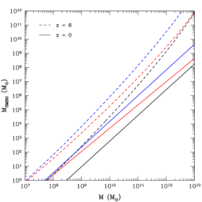
Figure 1: $M_{SMBH}$ as a function of the host halo mass $M$ at $z=6$ (dashed lines) and $z=0$ (solid lines). The three relations in Eq. (1) $(a)$-$(c)$ are shown from bottom to top for both redshifts.

The $M_{SMBH}$ obtained at $z=0$ is subsequently placed in halos at $z=z_{BH}$. For a fixed halo mass, SMBH at $z=0$ is less massive than SMBH at $z=6$. This is because the halos at $z=6$ would have evolved to a more massive halo by $z=0$, where the $M_{SMBH}$ is determined.

II.2 Formation and evolution of DM Spikes

The growth of SMBHs inevitably affects the surrounding distribution of DM. In fact, it can be shown that the adiabatic growth of a massive object at the center of a power-law distribution of matter with index $\gamma_{c}$, induces a redistribution of matter into a new, steeper, power-law with index $\gamma_{sp}=2+1/(4-\gamma_{c})$ peebles:1972 ; young:1980 ; Ipser:1987ru ; Quinlan:1995 ; Gondolo:1999ef . Such a DM enhancement is usually referred to as a “spike”. For the widely adopted Navarro, Frenk and White (NFW) profile (see Appendix for further comments and references), $\gamma_{c}=1$, and the spike profile, immediately after its formation (i.e. at $t=t_{f}$, the time when the spike is formed), can be expressed as

$$\rho_{sp}(r,0)=\rho(r_{b,0})\left(\frac{r}{r_{b,0}}\right)^{-7/3}$$ (2)

inside a region of size $r_{b,0}\approx 0.2\,r_{h}$ Merritt:2005yt , where $r_{h}$ is the radius of gravitational influence of the SMBH that is defined as

$$r_{h}\,\equiv\,{GM_{SMBH}\over\sigma^{2}}\,,$$ (3)

where $G$ is Newton’s constant and $\sigma$ the one-dimensional velocity dispersion. $M_{SMBH}$ can be related to $\sigma$ through the empirical relation ff05

$${M_{SMBH}\over 10^{8}\,M_{\odot}}\,=\,(1.66\pm 0.24)\,\left({\sigma\over 200\,\textrm{km s}^{-1}}\right)^{4.86\pm 0.43}\,.$$ (4)

Eq. (4) is known to be valid for SMBHs in the mass range $10^{6.5}M_{\odot}\lesssim M_{SMBH}\lesssim 10^{9.5}M_{\odot}$ and may extend to higher and lower masses ff05 .

Once the spike is formed, several particle physics and astrophysical effects tend to destroy it (e.g. Ullio:2001fb ; Merritt:2003qk ; Bertone:2005hw ; Bertone:2005xv ). Here we focus on the gravitational interaction between DM and stars near the SMBH, which causes a damping of the spike, and on self-annihilation of DM near the SMBH, which decreases the maximum density of the spike.

The DM and baryons gravitationally interact with each other. Stars in galactic nuclei have much larger kinetic energies than DM particles, and gravitational encounters between the two populations tend to drive them toward mutual equipartition. DM is thus heated up, dampening the spike while maintaing roughly the same shape of the density profile. Based on the results in Refs. Merritt:2003qk ; Bertone:2005hw , we adopted the following approximate expression for the decay of the spike intensity with time:

$$\rho(r,t)\,\approx\,\rho(r,0)\,\kappa\,;~{}~{}~{}~{}\kappa\equiv e^{-\tau/2}\,,$$ (5)

where $\tau$ is the time since spike formation in units of the heating time $T_{heat}$ Merritt:2003qk

$$T_{heat}\,=\,1.25{\rm Gyr}\,\times\\ \left({M_{SMBH}\over 3\times 10^{6}M_{\odot}}\right)^{\frac{1}{2}}\left({r_{h}\over 2{\rm pc}}\right)^{\frac{3}{2}}\left({M_{\odot}\over\tilde{m}_{\star}}\right)\left({15\over\ln\Lambda}\right).$$ (6)

$\tilde{m}_{\star}$ is the effective stellar mass, and is equal to $\sim 1.8M_{\odot}$ assuming a Salpeter mass function and $0.08M_{\odot}\leq m_{\star}\leq 20M_{\odot}$. $\ln\Lambda=\ln(0.4N)$, with $N\approx 6\times 10^{6}$ the number of stars within $r_{h}$ for our Milky Way Galaxy. Although $r_{h}$ is a function of $M_{SMBH}$, we approximate $\ln\Lambda$ to be constant as $T_{heat}$ dependence on $N$ is logarithmic.

The size of the spike decreases, with respect to the initial value $r_{b,0}$, with time

$$r_{b}(t)\,=\,\kappa^{\delta}\,r_{b,0}\,,~{}~{}~{}\delta\,\equiv\,(\gamma_{sp}-\gamma_{c})^{-1}\,.$$ (7)

The spike density profile is thus given as

$$\rho_{sp}(r,t)\,=\,\rho_{sp,0}\,\kappa^{\epsilon}\,\left({r\over r_{b}}\right)^{-\gamma_{sp}}~{},~{}~{}~{}\epsilon\equiv\gamma_{c}/(\gamma_{c}-\gamma_{sp})\,.$$ (8)

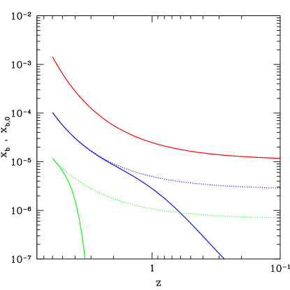
Figure 2: Redshift evolution of the spike parameters $x_{b}$ (solid lines) and $x_{b,0}$ (dotted lines), for various halo masses: $M_{h}(z_{BH})=10^{13},~{}10^{12},~{}10^{11}~{}M_{\odot}$ from top to bottom (red, blue, green), and assuming $z_{BH}=6$.

Figure 2 shows the spike evolution under the effect of DM interaction with baryons, assuming $z_{BH}=6$ for different halo masses. The spike parameters are shown in units of the halo reference radius $r_{0}$ (defined in Sec. A), so that $x_{b}\equiv r_{b}/r_{0}$ and $x_{b,0}\equiv r_{b,0}/r_{0}$. It can be seen that spikes formed in very massive halos are not affected by heating from the baryons, whereas those in less massive halos quickly dissipate. Hence low mass halos give negligible contribution to the gamma-ray signal.

A robust lower limit on the size of the spike is provided by the last stable orbit ($r_{lso}$) of a test particle around the SMBH. However, annihilation itself sets an upper limit on the DM density. The evolution equation of DM particles at radius $r$ and time $t$ is

$$\dot{n}_{sp}(r,t)\,=\,-\langle\sigma v\rangle\,n_{sp}(r,t)^{2}\,,$$ (9)

where the dot denotes a time derivative. Although this expression is correct for circular orbits, a more sophisticated approach would take into account the eccentricities of orbits, and would start from the single-particle distribution function $f(E,L)$ describing the DM particles, where $E$ and $L$ are the energy and angular momentum per unit mass respectively, and compute orbit-averaged annihilation rates. Such a calculation has apparently never been carried out and is beyond the scope of this paper. Under the assumption of circular orbits, one finds that the maximum number density at a given time $t$ can be expressed as

$$n_{sp}(r,t)\,=\,{n_{sp}(r,t_{f})\over 1\,+\,n_{sp}(r,t_{f})\,(t-t_{f})\,\langle\sigma v\rangle}\,.$$ (10)

This is usually simplified to obtain a maximum density

$$\rho_{pl}(t)\,\approx\,{m_{\chi}\over\langle\sigma v\rangle}{1\over(t-t_{f})}$$ (11)

The radius where $\rho_{sp}$ reaches this value, denoted as $r_{p}$, can be calculated by inserting Eq. (8) into the above equation. The maximum allowed density decreases with time due to self-annihilation and a plateau of constant density forms from $r_{p}$ down to $r_{lso}$. As $r_{min}$ is larger than $r_{lso}$, except for very massive halos, the fully evolving spike density profile is given as

$$\displaystyle\rho_{sp}(r,t)\,=\,\begin{cases}\rho_{pl}(t)&\,(r_{lso}\,<\,r\,\leq\,r_{p})\\ \rho_{sp,0}\,\kappa^{\epsilon}\,\left({r\over r_{b}}\right)^{-\gamma_{sp}}&\,(r_{p}\,<\,r)\end{cases}.$$ (12)

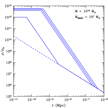
Figure 3: Density profile of an evolving spike. Halo and SMBH mass are fixed at $10^{12}\,M_{\odot}$ and $10^{7}\,M_{\odot}$, respectively, at all redshifts, and $z_{BH}=6$. The dashed line is the halo profile, and solid lines are the spike profile in various stages of evolution. Spikes are plotted at $\tau=\,1,~{}2,~{}3,$ and $\approx 14\,(z=0)$, from right to left (in order of decreasing size). The spike becomes prominent at $r_{b}(t)$, which decreases with time due to DM-baryon scattering. Self-annihilation of DM causes the maximum spike density value of $\rho_{pl}$ to decrease with time. A constant density of DM with value $\rho_{pl}$ is maintained from $r_{p}$ to the last stable orbit ($\sim 10^{-12}$ Mpc).

Figure 3 shows the density profile of an evolving spike which has formed at $z_{BH}=6$. Note that the evolution of the halo itself has not been taken into account and the halo and SMBH mass are fixed to $10^{12}\,M_{\odot}$ and $10^{7}\,M_{\odot}$, respectively, at all redshifts in order to show only the changes due to the evolving spike. The halo profile is plotted in dashed line and the spike profiles at various $\tau$s are plotted in solid lines. The DM profile is divided into three regions; a plateau with magnitude $\rho_{pl}$ from $r_{lso}$ to $r_{p}$, the prominent spike that scales as $r\sim r^{-\gamma_{sp}}$ from $r_{p}$ to $r_{b}$, and the prominent halo with $r\sim r^{-\gamma_{c}}$ from $r_{b}$ to $r_{v}$. Numerical computations, such as Ref. Bertone:2005hw which has been calculated for our Galaxy, show the same features but with a smoother transition at $r_{b}$.

It is convenient to express $\rho_{sp,0}$ in terms of $r_{0}$ and $\rho_{0}$, thus of halo mass. Given the halo mass $M$, one can obtain $r_{v}$ from Eq. (22) and $r_{0}$ from the definition of $c$ of Eq. (27). It should be noted that $r_{0}$ is not a constant but varies with $z$ and $M$. Similarly, $\rho_{0}$, which is also dependent on $z$ and $M$, is obtained by solving

$$M\,=\,4\,\pi\int^{r_{v}}_{0}dr\,r^{2}\rho_{h}(r)\,.$$ (13)

The reference spike density $\rho_{sp,0}$ is normalized by the halo density at $r=r_{b,0}$ and $\tau=0$. For a NFW halo this gives

$$\rho_{sp,0}\,=\,{\rho_{0}\over x_{b,0}\,(1\,+\,x_{b,0})^{2}}\,,$$ (14)

where $x_{b,0}\equiv r_{b,0}/r_{0}$, thus

$$\rho_{sp}(x)\,=\,\rho_{0}\,{x_{b,0}^{\gamma_{sp}-1}\over(1+x_{b,0})^{2}}\,\kappa\,x^{-\gamma_{sp}}\,.$$ (15)

The expression of the total density profile depends on the redshift and radius. The total density profile is given as follows:

$$\rho_{tot}\,=\,\begin{cases}\rho_{h}(r)&(z>z_{BH})\\ \rho_{h}(r)&(z\leq z_{BH},~{}r>r_{b})\\ \rho_{h}(r)\,+\,\rho_{sp}(r,t)&\\ ~{}~{}~{}~{}\approx\rho_{sp}(r,t)&(z\leq z_{BH},~{}r\leq r_{b})\end{cases}\,.$$ (16)

III Gamma-Ray background from DM annihilations

The contribution of DM annihilations to the gamma-ray background flux $\Phi$ can be expressed as  Bergstrom:2001jj

$$\Phi(E)\,=\,{c\over 4\,\pi}{1\over H_{0}}{\langle\sigma v\rangle\over 2}\left({\Omega_{m}\,\rho_{c}\over m_{\chi}}\right)^{2}\,\times\\ \int dz\,{(1+z)^{3}\over h(z)}{dN(E_{s})\over dE_{s}}e^{-\tau(z,E)}\zeta(z)\,,$$ (17)

where $c$ here is the speed of light, $H_{0}$ is the present value of the Hubble parameter, $E_{s}=E(1+z)$ is the energy emitted at the source, and $h(z)=\sqrt{(1+z)^{3}\Omega_{m}\,+\,\Omega_{\Lambda}}$. To allow an easy comparison with existing literature, we adopt a simple analytic fit to the continuum gamma-ray flux emitted per annihilation coming from hadronization and $\pi^{0}$ decay Bergstrom:2001jj

$${dN(E)\over dE}\,\approx\,{0.42\over m_{\chi}}\,{e^{-8{E/m_{\chi}}}\over(E/m_{\chi})^{1.5}\,+\,0.00014}\,,$$ (18)

which is valid for $E\leq m_{\chi}$. The exponential in the integrand takes into account the effect of gamma-ray absorption due to pair production on background photons. Following Bergstrom:2001jj , we write it as

$$e^{-\tau(z,E)}\,\approx\,\exp\left[\frac{-z}{3.3\,(E/10\,{\textrm{GeV}})^{-0.8}}\right]\,.$$ (19)

The dimensionless flux multiplier $\zeta(z)$ can be written as the integral over all masses of an auxiliary function $g(M,z)$, weighted by the halo mass function $dn/dM$, which is typically calculated in the framework of the Press-Schechter or Sheth-Tormen formalisms described in Sec. A.2,

$$\zeta(z)\,=\,\int dM\,{dn\over dM}\,g(M,z)\,.$$ (20)

The auxiliary function $g(M,z)$ is simply the flux multiplier relative to a halo of mass $M$ at redshift $z$,

$$g(M,z)\,=\,{1\over(\rho_{c}\Omega_{m})^{2}}\int_{V}dV\,\rho^{2}(r)\,,$$ (21)

normalized to the comoving background density squared. $V$ is the halo virial volume, which is a function of redshift, and of the halo mass and concentration (see Eq. (22)).

The integration over DM spikes requires particular care. Since we are assuming that SMBHs do not evolve after their formation redshift $z_{BH}$, the halo parameters in the $\zeta(z)$ calculation have to be evaluated at $z_{BH}$, while the spike evolves with redshift as discussed above. Furthemore, the $M-M_{SMBH}$ relationship must evidently break down at small masses. Here we have restricted the anlysis to spikes produced by BHs with mass $M_{SMBH}\geq 100\,M_{\odot}$, and have verified that the result is insensitive to this lower mass cutoff.

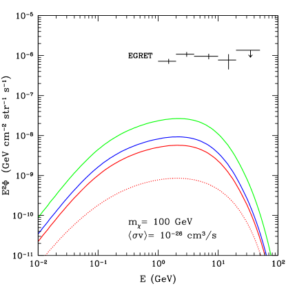
Figure 4: Gamma-ray background produced by DM annihilations in DM halos with spikes (solid lines), compared to the halo-only contribution (dotted). The EGRET diffuse flux limits Strong:2004ry are shown for comparison. Halos have mass between $10^{5}-10^{14}\,M_{\odot}$ and are distributed according to the Press-Schechter formalism. The three expressions in Eq. (1) are used for the $M_{SMBH}$-$M$ relation: $(a)$ (red) $(b)$ (blue) $(c)$ (green) from the bottom to top. The DM parameters adopted are $m_{\chi}=100$ GeV, $\langle\sigma v\rangle=10^{-26}\textrm{cm}^{3}\textrm{s}^{-1}$.

Figure 4 shows the enhancement of the gamma-ray background due to the presence of spikes, compared with the standard calculation (halo only). For the figure, we have focused on the Press-Schechter formalism, but we find similar results for the case of ellipsoidal collapse à la Sheth & Tormen. We given an upper limit of $z=18$ to Eq. (17) and assume that spikes form at $z_{BH}=2$. DM parameters $m_{\chi}=100$ GeV, $\langle\sigma v\rangle=10^{-26}~{}\textrm{cm}^{3}\textrm{s}^{-1}$ are used in the calculation. All three mass relations between the SMBH and halo of Eq. (1) are shown in the figure, $(a)$ to $(c)$ from bottom to top in solid lines. The diffuse EGRET flux Strong:2004ry is plotted as a comparison. Enhancement due to the presence of evolving spikes is about $\gtrsim$ order of magnitude. The evolving spike gives the largest enhancement to the overall flux at the lower energy region, while there is little enhancement at high energies close to $m_{\chi}$. This is expected, as the spikes are most prominent just after formation at $z_{BH}$, and gamma-rays emitted then have been redshifted to lower energies. Except for massive halos, most spikes today have died away and contribute very little to the gamma-ray flux. This also implies that the annihilation signal from the GC is not expected to vary significantly from the case of profiles without spikes.

We also consider a case where gamma-rays are emitted from annihilation of neutralinos into two photons. The photon flux is described as a delta function where $dN(E)/dE=b_{\gamma\gamma}\delta(E-m_{\chi})$, with $b_{\gamma\gamma}=0.003$ Bergstrom:2001jj . Considering only a delta function as the flux source is helpful to understand the enhancement due to the presence of spikes.

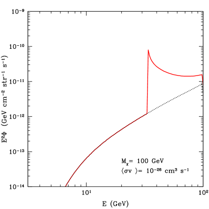
Figure 5: Gamma-ray flux due to annihilation of neutralinos into two photons. Halos have mass between $10^{5}-10^{14}\,M_{\odot}$ and are distributed according to the Press-Schechter formalism. Flux from halo only are shown in black dotted line, and flux from halo and evolving spike are shown in red solid line. Spikes give the greatest contribution at low energies, i.e. at high redshifts.

The spike is expected to give the largest contribution around $z_{BH}$, which today will be observed as gamma-rays with energy lower than $m_{\chi}$. Figure 5 shows the flux from annihilation into two photons for halo only and halo and spike contributions, and indeed, the largest enhancement comes at low energies. We have again assumed that halos form at $z=18$ and spikes form at $z_{BH}=2$ and used the $M-M_{SMBH}$ relation Eq. (1)-(a). The steep enhancement for the spike’s flux at $E\approx 30$ GeV is due to our assumption of having a fixed SMBH formation epoch ($z_{BH})$ and only using the delta function for the gamma ray flux.

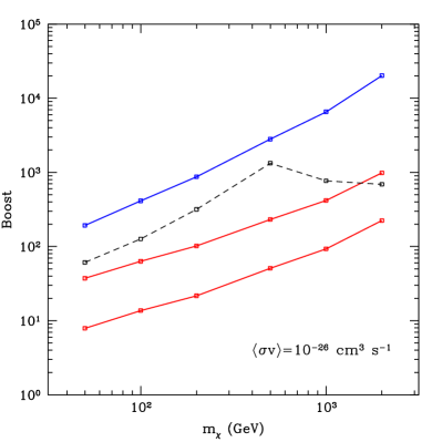
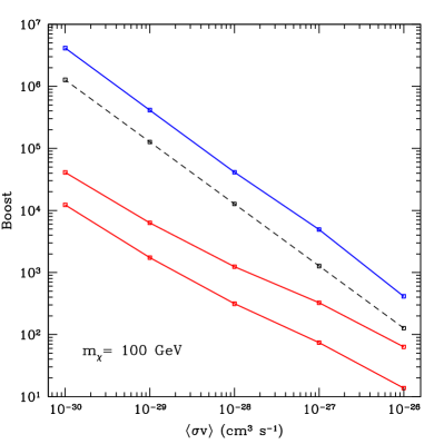
Figure 6: Required boost factor to match the EGRET background measurements with DM annihilations, for the halo only case (top blue solid line); halo+spike with $M_{SMBH}-M$ relation (a) (middle red solid line); and halo+spike with $M_{SMBH}-M$ relation (c) (lower red solid line). Halos have mass between $10^{5}-10^{14}\,M_{\odot}$ and are distributed according to the Press-Schechter formalism. Left panel: $m_{\chi}$ varies while the cross section is fixed at $\langle\sigma v\rangle=10^{-26}\textrm{cm}^{3}\textrm{s}^{-1}$. Right panel: $\langle\sigma v\rangle$ varies with a constant $m_{\chi}=100$ GeV. For comparison, we show the boost factor relative to the gamma-ray source at the GC (dashed line), using a NFW profile. Both EGRET and HESS observations are used.

To compare with existing literature, we introduce here a “boost factor” $b_{max}$ defined as in Ref. Ando:2005hr , i.e. $b_{\rm max}\equiv\min_{i}[\Phi_{\rm EGRET}(E_{i})/\Phi(E_{i})]$, where $\Phi_{\rm EGRET}$ is the EGRET flux measurement (Ref. Strong:2004ry for the diffuse background, and Refs. Mayer-Hasselwander98 ; Hartman:1999fc for the GC) relative to the energy bin $E_{i}$. We show in Fig. 6 the required boost factor for 3 different cases: halo only (top solid line), and halo+spike with 2 different assumptions for the $M_{SMBH}$-$M$ relation (lower solid lines). The left panel shows a constant $\langle\sigma v\rangle=10^{-26}\textrm{cm}^{3}\textrm{s}^{-1}$ with varying $m_{\chi}$ and the right panel shows a constant $m_{\chi}$ with varying $\langle\sigma v\rangle$. The boost factor for the GC is also shown as a comparision in dashed lines, where the HESS GC observation Aharonian:2004wa has also been considered. As one can see, for the $M_{SMBH}$-$M$ relation of Eq. (1)-(c), the required boost factor for the gamma-ray background is smaller than for the GC for most cases. We recall here that the spike contribution scales differently with the particle physics parameters $m_{\chi}$ and $\langle\sigma v\rangle$ with respect to the halo only case, due to the saturation effects produced by annihilation itself. In order for annihilations to contribute significantly to the observed gamma-ray background, a boost factor of at least 2 orders of magnitude is thus required. This could in principle be achieved by steepening the halo slope in the innermost regions, for e.g. due to adiabatic compression of baryons (see e.g. Ref. Bertone:2005xv and references therein), or to the presence of mini-spikes around intermediate mass black holes Bertone:2006nq ; Bertone:2005xz . One should however bear in mind that astrophysical sources are expected to provide a significant, possibly dominant, contribution to the background. Furthermore, the estimate of the background measured by EGRET has actually been recently questioned by several authors. We discuss in the next section the uncertainties on the EGRET measurements and on the possible astrophysical intepretation, and in light of these uncertainties, we do not attempt to fit the background with a combination of particle physics and halo models, and limit ourselves to point out the importance of the role played by spikes in the estimates of the DM annihilation contribution to the extra-galactic flux.

In Figs. 4-6 we have assumed a common redshift of formation for all SMBHs. We show in Fig. 7 the dependence of the gamma-ray background on the parameter $z_{BH}$: the left panel shows the evolution of $\zeta(z)$ (Eqn. (20)) for different values of $z_{BH}$, and the right panel shows the gamma-ray background. Younger spikes give a greater contribution to the gamma-ray background because of a larger $\zeta(z)$. The normalization of the annihilation signal has a slight dependence on $z_{BH}$, where small $z_{BH}$ values give larger contribution to the gamma-ray flux. This is expected as spikes that formed in earlier epochs evolve away with time.

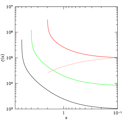
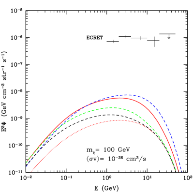
Figure 7: Left panel: $\zeta(z)$ for spikes (solid lines), assuming from bottom to top, $z_{BH}=$ 6 (black), 4 (green), 2 (red). The halo $\zeta_{z}$ corresponding to the halo-only contribution is shown for comparion (dotted line). Right panel: Sensitivity of the predicted gamma-ray background to the formation redshift of SMBHs, $z_{BH}$, compared with $z_{BH}=2$ case used in previous figures. The lower dotted line represents the contribution of the halo only, the four upper curves dashed and solid lines indicate the halo+spike contribution for the $M_{SMBH}$-$M$ relation $(a)$ with, $z_{BH}=$ 6 (black), 4 (green), 2 (red solid), 1 (blue) from bottom to top. Halos have mass between $10^{5}-10^{14}\,M_{\odot}$ and are distributed according to the Press-Schechter formalism.

On the other hand, dependence on halo formation redshift is negligible; changing the upper limit on redshift fro Eq. (17) from 18 to 12 brings negligible change for both halo and halo+spike gamma-ray flux. The flux has a small dependence on the maximum halo mass: a $10^{13}\ M_{\odot}$ limit lower the flux by $<$ 20 %. Varying the minimum halo mass brings negligible change.

All calculations so far assumed that spikes never experienced a major merger, which could in principle significantly lower the DM density due to the souring effect of binary BHs Merritt:2002vj . To model the effect of galaxy mergers on the annihilation signal, we used the merger tree model of Ref. Wechsler:2001cs (Eq. (39)), and assume that a galaxy merger occured and its spike destroyed at $z_{m}$ when its halo mass at $z_{BH}$ doubles, i.e., $M(z_{m})=2M(z_{BH})$. Figure 8 shows the effect merger has on the gamma-ray signals produced by spikes. The solid lines are the spike+halo contribution without mergers, and the dashed lines are the spike+halo contribution with merger taken into account. The dotted line is the halo contribution only, shown for comparison. Three redshifts are considered, $z_{BH}=$ 2, 4, 6, which gives a $z_{m}=$ 0.88, 2.12, 3.37, respectively.

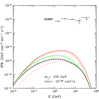
Figure 8: Gamma-ray background produced by DM annihilations in spikes including (dashed lines) and neglecting (solid lines) the effect of mergers. Three redshifts of formation have been considered for SMBHs; $z_{BH}=$ 2 (red, top lines), 4 (green, middle lines), 6 (black, lower lines). The dotted line represents the halo contribution. Halos have mass between $10^{5}-10^{14}\,M_{\odot}$ and are distributed according to the Press-Schechter formalism.

The reason for such small effect of mergers can be seen from the left panel of Fig 7; most of the contribution from the spikes come right after its formation. By the time of the merger, most spikes would be already quite small and not give significant contribution to the gamma-ray background.

IV Discussion and conclusions

Different strategies have been proposed in the literature to search for DM annihilation radiation. One of the most popular targets of indirect DM searches is the GC. The prospects for detecting gamma-rays from DM annihilations at the GC have been discussed extensively in Refs. Bouquet:1989sr ; Stecker:1987dz ; Berezinsky:1994wv ; Bergstrom:1997fj ; Cesarini:2003nr ; Bertone:2002ms ; Cheng:2002ej for DM cusps in the framework of different DM candidates, and in Refs. Bertone:2002je ; Bertone:2005hw ; Bertone:2005xv for the case of a DM spike at the GC. An updated discussion in light of the recent discovery of a point source coincident with the GC, extending to very high energies can be found in Refs. Hooper:2004vp ; Profumo:2005xd ; Mambrini:2005vk ; Zaharijas:2006qb . Current data do not allow a convincing interpretation of the gamma-ray emission as due to DM annihilation, while the properties of the gamma-ray emission appear consistent with those expected for an ordinary astrophysical source. However, although the DM intepretation of the gamma-ray source at the GC appears problematic, it can certainly be used in a conservative way to set upper limits on the annihilation signal. Alternatively, one could search for the contribution of DM annihilations to the cosmological gamma-ray background, as discussed in Refs. Bergstrom:2001jj ; Taylor:2002zd ; Ullio:2002pj ; Elsaesser:2004ck ; Elsaesser:2004ap ; Ando:2005hr ; Oda:2005nv . The “smoking-gun” in this case may come from the peculiar angular power spectrum predicted for this signal Ando:2005xg .

The predicted gamma-ray background is usually compared with the extra-galactic emission measured by EGRET Sreekumar:1997un . The most convincing interpretation in terms of conventional astrophysical sources invokes a large contribution from unresolved blazars (e.g. Ref. Stecker:1996ma ), although this conclusion has been challenged by other authors (e.g. Refs. Mukherjee:1999it ; mucke ). An additional contribution may arise from Inverse Compton scattering of electrons accelerated at shocks during structure formation Colafrancesco:1998us ; Totani:2000rg ; Loeb:2000na , but this process can hardly account for the bulk of the background Gabici:2002fg . The EGRET extra-galactic background should however be treated with caution, since it has been inferred (not measured) by substracting the estimated Galactic foreground from the high latitude EGRET measurements. In a recent re-analysis of the EGRET data, Kehet et al. Keshet:2003xc , noticed that the high latitude profile of the gamma-ray data exhibits strong Galactic features and claimed that it is well fit by a simple Galactic model, obtaining an upper limit on the extra-galactic background 3 times stronger than previously assumed, and evidence for a much lower flux. In light of the large uncertainties associated with the data and with the contribution of conventional astrophysical sources, we conservatively consider the EGRET estimate as an upper limit to the actual gamma-ray background, and do not attempt to fit the data with an ad hoc combination of particle physics and halo properties.

A comparison of the two strategies (GC vs. extra-galactic background) has been performed in Ref. Ando:2005hr , where it was shown that for ordinary cusps, and in particular for an NFW profile, the prospects for detecting gamma-rays from the GC are always more promising than for the gamma-ray background. Here we have shown that the situation changes, if we take into account the formation and evolution of DM spikes, which form due to adiabatic growth of SMBHs at the centers of DM halos. In fact, in this picture a spike inevitably develops also at the center of the Galaxy, but it is rapidly destroyed by the combined effect of DM scattering off stars, and DM annihilations themselves. The enhancement of the annihilation signal is thus negligible Bertone:2005hw ; Bertone:2005xv .

We have shown here that the opposite is true for the gamma-ray background. In fact, although all spikes are affected by the very same processes, the signal in this case receives contributions also from halos at high redshift, at a time when astrophysical and particle physics processes did not yet have the time to affect the DM density. As a consequence, the gamma-ray background from DM annihilations receives a substantial boost, so that its detectability is in some scenarios more promising than the case of a gamma-ray source at the GC. An additional reason to consider the gamma-ray background as a valid alternative to GC searches, is that it is sensitive to the average properties of halos, whereas in the GC case one has to deal with a single realization that, as far as we know, may differ significantly from the average, given the significant scatter in the properties of halos observed in numerical simulations, and given the unknown history of the baryons.

Several effects could further boost the annihilation background. One possibility is that DM halos undergo “adiabatic contraction” under the influence of baryons, thus steepening the original DM profile (see e.g. Bertone:2005xv and references therein), a circumstance that would lead to a similar boost of both the background and GC fluxes. Conversely, if mini-spikes of DM around intermediate mass black holes exist Bertone:2006nq ; Bertone:2005xz , this would have dramatic implications for the predicted annihilation background, while leaving practically unchanged the predictions for the GC Horiuchi:2006de .

V Acknowledgements

We thank S. Ando, P. Natarajan, L. Pieri, G. Sigl, R. Somerville, M. Volonteri, and the anonymous referee for useful comments. The work of EJA was supported in part by NSF PHY-0114422. KICP is a NSF Physics Frontier Center. The work of EJA is now supported by the U.S. Department of Energy under Contract No. DE-FG02 91ER 40626. The work of GB and PJZ was supported at an earlier stage of the collaboration by the DOE and NASA grant NAG 5-10842 at Fermilab. GB is now supported by the Helmholtz Association of National Research Centres. This research was supported in part by the National Science Foundation under grants no. PHY99-07949, AST-0206031, AST-0420920 and AST-0437519, by the National Aeronautics and Space Administration under grant no. NNG04GJ48G, and by the Space Telescope Science Institute under grant no. HST-AR-09519.01-A to DM.

Appendix A Properties of DM Halos

We present here our prescription to calculate DM density profiles $\rho_{h}(r)$, for halos of mass $M$ and redshift $z$, and the dimensionless flux multiplier $\zeta(z)$, that we used for the calculation of the gamma-ray background. For the sake of completeness, we explicitly write all the ingredients of the calculation, with relevant references, also to allow the comparison with exisiting literature.

A.1 Halo density profile

The virial mass $M$ of a DM halo can be expressed in terms of the virial radius $r_{v}$ as

$$M\,=\,{4\pi\over 3}\,r_{v}^{3}\,\Delta_{c}\,\rho_{c}\,,$$ (22)

where $\rho_{c}$ is the critical density and $\Delta_{c}$ is the virial overdensity, that for a flat $\Lambda$CDM cosmology can be approximated by Bryan:1997dn

$$\Delta_{c}\,=\,18\pi^{2}\,+\,82(\Omega_{m}(z)-1)\,-\,39(\Omega_{m}(z)-1)^{2}\,.$$ (23)

Here, $\Omega_{m}(z)$ is the matter density in units of $\rho_{c}$.

N-body simulations suggest that the density of DM follows a universal profile, usually parametrized as Bergstrom:2000pn ; Bertone:2004pz

$$\rho_{h}(r)\,=\,\rho_{0}\,{r_{0}^{\alpha\,+\,\beta\gamma}\over r^{\alpha}\,(r^{\beta}\,+\,r_{0}^{\beta})^{\gamma}}\,.$$ (24)

where $\rho_{0}$ and $r_{0}$ set the normalization of the density and radius, respectively. We adopt here the so-called Navarro, Frenk and White (NFW) profile Navarro:1996gj , which can be obtained from the above parametrization with the following choice of parameters $\alpha=\beta=1,~{}\gamma=2$. In this case, the profile reduces to

$$\rho_{NFW}(x)\,=\,{\rho_{0}\over x\,(1\,+\,x)^{2}}\,,$$ (25)

where $x\equiv r/r_{0}$. The reference density $\rho_{0}$ can be expressed in this case as

$$\rho_{0}\,=\,{1\over 4\pi}\,{M\over r_{0}^{3}}\,{1\over\ln(1+c)-c/(1+c)}\,,$$ (26)

where $c$ is an adimensional concentration parameter

$$c\,\equiv\,{r_{v}\over r_{0}}\,.$$ (27)

Although subsequent studies have refined the description of DM halos with respect to the NFW profile, and more recent parametrizations of the innermost regions of galactic halos appear better suited to capture the behavior in the small-radii limit (see e.g. Navarro:2003ew ; Reed:2003hp ), we present our results for the NFW profile, which has emerged over the years as a benchmark model for DM annihilation studies. The scenario and prescriptions described here, however, can easily be extended to any DM profile.

A convenient expression for $c$ at redshift $z$ for halo mass $M(z)$ was derived in Ref. Bullock:1999he from a statistical sample of high-resolution N-body simulations, containing $\approx 5000$ halos in the range $10^{11}-10^{14}\,M_{\odot}$:

$$c\,=\,{9\over 1+z}\,\left({M(z)\over M_{\star}(z=0)}\right)^{-0.13}\,.$$ (28)

The collapse mass $M_{\star}(z)$ defines the mass that collapses to form at halo at redshift $z$. For $\Lambda$CDM cosmology, $M_{\star}(z=0)\simeq 1.5\times 10^{13}\,h^{-1}\,M_{\odot}$. A detailed way of obtaining $M_{\star}$ is described in Sec. A.3. Concentration parameters of halos less massive than $\sim 10^{10}M_{sun}$ have not been robustly measured in N-body simulations, due to the required mass and force resolution. For concreteness, we assume Eq. (28) to apply for any halos. The validity of extrapolating Eq. (28) to small halos should be tested against future simulations.

A.2 Halo mass distribution

In this subsection, we discuss another key ingredient for the calculation of the cosmological annihilation flux. We need now to specify the mass function of DM halos, i.e. the number of objects of given mass M. The mass function of halos are expressed in a universal form Press:1973iz

$${dn\over dM}\,=\,{\rho_{M}\over M}\,{d\nu\over dM}\,f(\nu)\,,$$ (29)

where $\rho_{M}=\rho_{c}\Omega_{M}$ is the comoving matter (background) density and a new variable $\nu$ is defined

$$\nu\,\equiv\,{1.686\over D(z)\,\sigma(M)}\,.$$ (30)

The linear equivalent of the over density at collapse for spherical collapse model is 1.686, $\sigma(M)$ is the rms density fluctuation in a sphere with mass $M$, and $D(z)$ is the linear density growth rate.

In this way, $f(\nu)$ for spherical collapse is expressed as

$$f(\nu)\,=\,\sqrt{{2\over\pi}}\,e^{-\nu^{2}/2}\,.$$ (31)

A better fit to number density of halos can be obtained with the ellipsoidal collapse model derived by Sheth and Tormen Sheth:1999su ;

$$f(\nu)\,=\,A\sqrt{a}\,\left(1\,+\,{1\over{\nu^{\prime}}^{2q}}\right)\,\sqrt{{2\over\pi}}\,e^{{-\nu^{\prime}}^{2}/2}\,,$$ (32)

where $\nu^{\prime}=\sqrt{a}\nu$. Numerical fits to simulations give $a=0.707,~{}p=0.3$ Jenkins:1997en , and $A$ is obtained by normalising $f(\nu)$.

$\sigma(M)$ is related to the power spectrum $P(k)$ by

$$\sigma(M)^{2}\,\propto\,\int d^{3}k\,\tilde{W}(kR)^{2}\,P(k)\,,$$ (33)

where $k$ is the wave number and $\tilde{W}(kR)$ is the filter function with $R$ being the radius enclosing mass $M$. We choose a top-hat function for $\tilde{W}(kR)$;

$$\tilde{W}(y)\,=\,{3\over y^{3}}\,(\sin\,y\,-\,y\,\cos\,y)\,.$$ (34)

We adopt here a power spectrum

$$P(k)\,\propto\,k^{n}\,T(k)^{2}\,,$$ (35)

where the Bardeen-Bond-Kaiser-Szalay (BBKS) transfer function Bardeen:1985tr is used for $T(k)$:

$$T(k)\,=\,{\ln(1+2.34q)\over 2.34q}\,[1\,+\,3.89q\,+\,\\ (16.1q)^{2}+\,(5.46q)^{3}\,+\,(6.71q)^{4}]^{-1/4}\,,$$ (36)

with $q\equiv k/(\Omega_{m}h^{2})$ (Mpc). $P(k)$ and $\sigma(M)$ are normalized by simulating $\sigma(M)$ in spheres of $R=8/h$ Mpc, commonly known as $\sigma_{8}$. We use $\sigma_{8}=0.9$ from the concordance model.

Finally, we provide an expression for the linear growth rate $D(z)$ Carroll:1991mt , which can be expressed as

$$D(z)\,=\,{1\over 1+z}\,{g(z)\over g(0)}\,,$$ (37)

where

$$g(z)\,=\,{5\over 2}\,\Omega_{m}(z)\,\times\left[\Omega_{m}(z)^{4/7}\,-\,\right.\\ \left.\Omega_{\Lambda}\,+\left(1+{\Omega_{m}(z)\over 2}\right)\,\left(1+{\Omega_{\Lambda}\over 70}\right)\right]^{-1}\,.$$ (38)

A.3 Evolution of halos

In order to assign the appropriate BH mass to a host halo, we need to evolve back in time the halo mass, and calculate its mass at the redshift of formation of the SMBH. We follow the semi-analytic study of halo evolution with merger trees, carried out in Ref. Wechsler:2001cs , and express the halo mass at $z_{0}$ as a function of an earlier redshift $z_{1}$

$$M(z_{0})\,=\,M(z_{1})\,\exp\left[{S\over 1+z_{c}}\,\left({1+z_{1}\over 1+z_{0}}-1\right)\right]\,.$$ (39)

The free paramter $S$ is proportional to the logarithmic slope of accretion rate, $dlogM/da$ where $a=1/(1+z)$, and is usually set to 2. The collapse redshift $z_{c}$ is defined according to Ref. Bullock:1999he , where the collapse mass $M_{\star}$ is a fixed fraction of the halo mass $M$

$$M_{\star}(z_{c})\,=\,f\,M.$$ (40)

In $\Lambda$CDM cosmology, $f$ is typically 0.01. $M_{\star}(z)$ is defined such that $\sigma(M_{\star}(z),z)=1.686$, or equivalently, $\nu=1$. We solve the above equation to find $z_{c}$ for each M.

By setting $\nu=1$, we have

$$D(z_{c})\,=\,{1.686\over\sigma(M_{\star}(z_{c}))}\,=\,{1.686\over\sigma(0.01M)}\,.$$ (41)

Hence $z_{c}$ is obtained by interpolating the expression $D(z_{c})$ of Eq. (37).

References

- (1) L. Bergstrom, Rept. Prog. Phys. 63, 793 (2000), hep-ph/0002126.
- (2) C. Munoz, Int. J. Mod. Phys. A19, 3093 (2004), hep-ph/0309346.
- (3) G. Bertone, D. Hooper, and J. Silk, Phys. Rept. 405, 279 (2005), hep-ph/0404175.
- (4) L. Bergstrom, J. Edsjo, and P. Ullio, Phys. Rev. Lett. 87, 251301 (2001), astro-ph/0105048.
- (5) J. E. Taylor and J. Silk, Mon. Not. Roy. Astron. Soc. 339, 505 (2003), astro-ph/0207299.
- (6) P. Ullio, L. Bergstrom, J. Edsjo, and C. G. Lacey, Phys. Rev. D66, 123502 (2002), astro-ph/0207125.
- (7) S. Ando, Phys. Rev. Lett. 94, 171303 (2005), astro-ph/0503006.
- (8) D. Merritt, Memorie della Societa Astronomica Italiana. 77, 750 (2006), astro-ph/0602353.
- (9) P. J. E. Peebles, Astrophys. J. 178, 371 (1972).
- (10) P. Young, Astrophys. J. 242, 1232 (1980).
- (11) J. R. Ipser and P. Sikivie, Phys. Rev. D35, 3695 (1987).
- (12) G. D. Quinlan, L. Hernquist, and S. Sigurdsson, Astrophys. J. 440, 554 (1995), astro-ph/9407005.
- (13) P. Gondolo and J. Silk, Phys. Rev. Lett. 83, 1719 (1999), astro-ph/9906391.
- (14) P. Ullio, H. Zhao, and M. Kamionkowski, Phys. Rev. D64, 043504 (2001), astro-ph/0101481.
- (15) D. Merritt, Phys. Rev. Lett. 92, 201304 (2004), astro-ph/0311594.
- (16) G. Bertone and D. Merritt, Phys. Rev. D72, 103502 (2005), astro-ph/0501555.
- (17) G. Bertone and D. Merritt, Mod. Phys. Lett. A20, 1021 (2005), astro-ph/0504422.
- (18) G. Bertone, A. R. Zentner, and J. Silk, Phys. Rev. D72, 103517 (2005), astro-ph/0509565.
- (19) A. Soltan, Mon. Not. Roy. Astron. Soc. 200, 115 (1982).
- (20) Q.-j. Yu and S. Tremaine, Mon. Not. Roy. Astron. Soc. 335, 965 (2002), astro-ph/0203082.
- (21) M. Elvis, G. Risaliti, and G. Zamorani, (2001), astro-ph/0112413.
- (22) A. Marconi et al., Mon. Not. Roy. Astron. Soc. 351, 169 (2004), astro-ph/0311619.
- (23) L. Ferrarese, Astrophys. J. 578, 90 (2002), astro-ph/0203469.
- (24) A. Marconi and L. K. Hunt, Astrophys. J. 589, L21 (2003), astro-ph/0304274.
- (25) L. Ferrarese and H. Ford, Space Science Reviews 116, 523 (2005), astro-ph/0411247.
- (26) R. H. Wechsler, J. S. Bullock, J. R. Primack, A. V. Kravtsov, and A. Dekel, Astrophys. J. 568, 52 (2002), astro-ph/0108151.
- (27) D. Merritt and A. Szell, Astrophys. J. 648, 890 (2006), astro-ph/0510498.
- (28) A. W. Strong, I. V. Moskalenko, and O. Reimer, Astrophys. J. 613, 956 (2004), astro-ph/0405441.
- (29) H. A. Mayer-Hasselwander et al., Astron. Astrophys. 335, 161 (1998).
- (30) EGRET, R. C. Hartman et al., Astrophys. J. Suppl. 123, 79 (1999).
- (31) The HESS, F. Aharonian et al., Astron. Astrophys. 425, L13 (2004), astro-ph/0408145.
- (32) G. Bertone, Phys. Rev. D73, 103519 (2006), astro-ph/0603148.
- (33) D. Merritt, M. Milosavljević, L. Verde, and R. Jimenez, Phys. Rev. Lett. 88, 191301 (2002).
- (34) A. Bouquet, P. Salati, and J. Silk, Phys. Rev. D40, 3168 (1989).
- (35) F. W. Stecker, Phys. Lett. B201, 529 (1988).
- (36) V. Berezinsky, A. Bottino, and G. Mignola, Phys. Lett. B325, 136 (1994), hep-ph/9402215.
- (37) L. Bergstrom, P. Ullio, and J. H. Buckley, Astropart. Phys. 9, 137 (1998), astro-ph/9712318.
- (38) A. Cesarini, F. Fucito, A. Lionetto, A. Morselli, and P. Ullio, Astropart. Phys. 21, 267 (2004), astro-ph/0305075.
- (39) G. Bertone, G. Servant, and G. Sigl, Phys. Rev. D68, 044008 (2003), hep-ph/0211342.
- (40) H.-C. Cheng, J. L. Feng, and K. T. Matchev, Phys. Rev. Lett. 89, 211301 (2002), hep-ph/0207125.
- (41) G. Bertone, G. Sigl, and J. Silk, Mon. Not. Roy. Astron. Soc. 337, 98 (2002), astro-ph/0203488.
- (42) D. Hooper, I. de la Calle Perez, J. Silk, F. Ferrer, and S. Sarkar, JCAP 0409, 002 (2004), astro-ph/0404205.
- (43) S. Profumo, Phys. Rev. D72, 103521 (2005), astro-ph/0508628.
- (44) Y. Mambrini, C. Munoz, E. Nezri, and F. Prada, JCAP 0601, 010 (2006), hep-ph/0506204.
- (45) G. Zaharijas and D. Hooper, Phys. Rev. D73, 103501 (2006), astro-ph/0603540.
- (46) D. Elsaesser and K. Mannheim, Astropart. Phys. 22, 65 (2004), astro-ph/0405347.
- (47) D. Elsaesser and K. Mannheim, Phys. Rev. Lett. 94, 171302 (2005), astro-ph/0405235.
- (48) T. Oda, T. Totani, and M. Nagashima, Astrophys. J. 633, L65 (2005), astro-ph/0504096.
- (49) S. Ando and E. Komatsu, Phys. Rev. D73, 023521 (2006), astro-ph/0512217.
- (50) EGRET, P. Sreekumar et al., Astrophys. J. 494, 523 (1998), astro-ph/9709257.
- (51) F. W. Stecker and M. H. Salamon, Astrophys. J. 464, 600 (1996), astro-ph/9601120.
- (52) R. Mukherjee and J. Chiang, Astropart. Phys. 11, 213 (1999), astro-ph/9902003.
- (53) A. Mücke and M. Pohl, Mon. Not. Roy. Astron. Soc. 312, 177 (2000).
- (54) S. Colafrancesco and P. Blasi, Astropart. Phys. 9, 227 (1998), astro-ph/9804262.
- (55) T. Totani and T. Kitayama, Astrophys. J. 545, 572 (2000), astro-ph/0006176.
- (56) A. Loeb and E. Waxman, Nature 405, 156 (2000), astro-ph/0003447.
- (57) S. Gabici and P. Blasi, Astropart. Phys. 19, 679 (2003), astro-ph/0211573.
- (58) U. Keshet, E. Waxman, and A. Loeb, JCAP 0404, 006 (2004), astro-ph/0306442.
- (59) S. Horiuchi and S. Ando, Phys. Rev. D74, 103504 (2006), astro-ph/0607042.
- (60) G. L. Bryan and M. L. Norman, Astrophys. J. 495, 80 (1998), astro-ph/9710107.
- (61) J. F. Navarro, C. S. Frenk, and S. D. M. White, Astrophys. J. 490, 493 (1997), astro-ph/9611107.
- (62) J. F. Navarro et al., Mon. Not. Roy. Astron. Soc. 349, 1039 (2004), astro-ph/0311231.
- (63) D. Reed et al., Mon. Not. Roy. Astron. Soc. 357, 82 (2005), astro-ph/0312544.
- (64) J. S. Bullock et al., Mon. Not. Roy. Astron. Soc. 321, 559 (2001), astro-ph/9908159.
- (65) W. H. Press and P. Schechter, Astrophys. J. 187, 425 (1974).
- (66) R. K. Sheth, H. J. Mo, and G. Tormen, Mon. Not. Roy. Astron. Soc. 323, 1 (2001), astro-ph/9907024.
- (67) Virgo Consortium, A. Jenkins et al., Astrophys. J. 499, 20 (1998), astro-ph/9709010.
- (68) J. M. Bardeen, J. R. Bond, N. Kaiser, and A. S. Szalay, Astrophys. J. 304, 15 (1986).
- (69) S. M. Carroll, W. H. Press, and E. L. Turner, Ann. Rev. Astron. Astrophys. 30, 499 (1992).