Kinematic modelling of disk galaxies

This is the first of a series of papers in which the kinematics of disk galaxies over a range of scales is scrutinised employing spectroscopy.

A fundamental aspect of these studies is presented here: the new publicly available software tool TiRiFiC (http://www.astro.uni-bonn.de/~gjozsa/tirific.html) enables a direct fit of a “tilted-ring model” to spectroscopic data cubes. The algorithm generates model data cubes from the tilted-ring parametrisation of a rotating disk, which are automatically adjusted to reach an optimum fit via a chi-squared minimisation method to an observed data cube. The structure of the new software, the shortcomings of the previously available programs to produce a tilted-ring model, and the performance of TiRiFiC are discussed.

Our method is less affected by the well-known problem of beam smearing that occurs when fitting to the velocity field. Since with our method we fit many data points in a data cube simultaneously, TiRiFiC is sensitive to very faint structures and can hence be used to derive tilted-ring models significantly extending in radius beyond those derived from a velocity field. The software is able to parametrise H I disks of galaxies that are intersected by the line-of-sight twice or more, i.e. if the disks are heavily warped, and/or with a significant shift of the projected centre of rotation, and/or if seen edge-on. Furthermore, our method delivers the surface-brightness profile of the examined galaxy in addition to the orientational parameters and the rotation curve.

In order to derive kinematic and morphological models of disk galaxies, especially reliable rotation curves, a direct-fit method as implemented in our code should be the tool of choice.

1 Introduction

Kinematic analyses based on spectroscopy are an important tool to constrain the dynamical structure and hence the distribution of matter in galaxies. The discovery and description of global features in the kinematics of galaxies, such as the flatness of rotation curves (Rubin & Ford 1970; Bosma 1978), directly influenced cosmology. Since then, the increase of computational power enabled theorists to provide testable predictions on the mass distribution on sub-galaxy scales for given cosmological models (e.g. Navarro et al. 1997; Moore et al. 1999; Reed et al. 2005), such that kinematical studies can be utilised as immediate tests for cosmology. While in recent years the debate concentrated mainly on the spherical distribution of Dark Matter in relaxed systems (e.g. Swaters et al. 2003; de Blok et al. 2003; Gentile et al. 2004; Navarro et al. 2004), deviations from this, which are evident from lopsidedness (e.g. Schoenmakers et al. 1997) or warping (e.g. Bosma 1978), now come into the focus of theoretical research in the cosmological context (Sharma & Steinmetz 2005; Gao & White 2006). The aim to constrain the structure of anisotropies in the DM distribution imposes an observational challenge, requiring both observations with high sensitivity as well as appropriate analysis tools.

This is the first paper in a series with the aim to push forward the observational limits in order to put further constraints on theory, to gain insight in the large-scale structure of the disk-halo system in disk galaxies, and to further test proposed mass-density profiles. One of the major ingredients is the necessary development of improved analysis methods. A new software tool to analyse the kinematics of disk galaxies is presented in this paper.

It is known from observations that the orbits of the disk material in spiral galaxies without large bars have a comparably low ellipticity (e.g. Bosma 1981; Schoenmakers et al. 1997), such that it is a good approximation to treat them as being circular. This means that to first order the kinematics of a galactic disk at a certain galactocentric radius can be described by a set of three parameters, viz. the rotation velocity, and two parameters that describe the local disk orientation with respect to some reference system. Such a “tilted-ring model” was first constructed for M83 by Rogstad et al. (1974).

In some cases the tilted-ring model is an oversimplification, for example when the orbits are significantly non-circular due to the presence of a bar (e.g. Bosma 1978; Simon et al. 2003). Nevertheless, in many cases it serves as a good approximation and hence is the standard kinematic model for galaxies. Several algorithms exist to fit such a model to spectroscopic data. The most extensively used is the ROTCUR routine (van Albada et al. 1985; Begemann 1987), which is a generalisation of the original method of Warner et al. (1973). It is implemented in several data analysis packages, e.g. GIPSY (van der Hulst et al. 1992), NEMO (Teuben 1995) and AIPS (Fomalont 1981). ROTCUR fits a set of inclined rings to a velocity field. ROTCUR derivatives and extensions exist. The GIPSY routine RESWRI takes into account that non-axisymmetric potentials have a characteristic imprint on the velocity field (Binney 1978; Teuben 1991) and allows for any azimuthal variations of the rotation velocity (see also Franx et al. 1994; Schoenmakers et al. 1997). Similarly, RINGFIT (Simon et al. 2003) allows for the same variation, while at the same time only treating a flat disk. Simon et al. (2005) used this routine to test the reliability of their rotation curves. ROTCURSHAPE (implemented in NEMO, Teuben 1995) performs a global fit of the velocity field, in which the ring parameters are not fitted independently, but “in one go”. A reduction of the higher order terms in a harmonic expansion is used by KINEMETRY (Krajnović et al. 2006) in order to find the best fitting solution of a tilted-ring model.

All these routines have in common that they are based on an analysis of the velocity field, which itself is derived from a data cube, so it is an intermediate step when going from the observed data cube to a tilted ring model. Various methods exist to extract a velocity field by analysing the spectra in a data cube. All of these methods have their shortcomings. First, for galaxies with large warps or galaxies seen close to edge-on, the derivation of a single representative velocity field is impossible, because even if the disk geometry is known, the line-of-sight intersects the disk twice or more. This means that for some positions on the sky more than one velocity has to be inferred. Second, a velocity field is contaminated by beam smearing effects (see below, also Teuben 2002). The integration of emission along the line-of-sight in a thickened galaxy causes a similar effect. This leads to a situation where, in principle, a tilted-ring model resulting from a fit to a velocity field has to be cross-checked with a model data cube as can be produced by the GIPSY routine GALMOD (van der Hulst et al. 1992, originally designed by T.S. van Albada). Some authors have fitted such model data cubes by adjusting the model parameters and successively improving the model data cube by comparing it with the original data cube “by eye” (Arnaboldi & Galletta 1993; Swaters 1999; Gentile et al. 2004).

The drawbacks of just using the velocity field fits led to the development of a number of software tools that perform direct fits to the data cube (Irwin & Seaquist 1991) or to a position-velocity diagram (Simard & Pritchet 1999; Takamiya & Sofue 2002; Böhm et al. 2004), thus circumventing the beam-smearing or smoothing problem. These fit routines, which simulate an observation from a model parametrisation, do not allow, however, for an intrinsic change of the orientational parameters and hence are only limited implementations of the tilted-ring model. Especially for the analysis of H I kinematics, full 3D fitting is most suitable, and has first been implemented by Corbelli & Schneider (1997) and applied to the spiral galaxy M33. In this case, however, the fit was performed on single spectra resulting from a single-dish observation. Thus, besides not being available publicly, this algorithm would not suit to perform a fit to a data cube produced by synthesis or integral-field spectroscopic observations.

In this paper, the new, publicly available software called TiRiFiC (“Tilted-Ring-Fitting-Code”) is presented, which performs an automated fit of a tilted-ring model to a data cube. This software was originally developed to construct tilted-ring models of heavily warped galaxies observed in the H I emission line. It can, however, be used for all kinds of spectroscopic data cubes of translucent objects that can be approximated by the tilted-ring model. While the software will be under development for quite some time in order to improve the performance and to extend functionality beyond the classic tilted-ring model, TiRiFiC is well usable in its current form.

In this paper, we try to answer two basic issues: does a method to fit a tilted-ring model directly to the data cube lead to more reliable results than a fit to the velocity field and is it thus possible to reach a reasonable fit within a reasonable computational time? The paper is laid out as follows: in Sect. 2 the model layout and the fitting procedure are introduced, in Sect. 3 the smoothing effect of velocity field-based fitting algorithms is discussed, in Sect. 4 the results of a few tests of TiRiFiC are presented. In Sect. 5 the results are summarised. First applications of TiRiFiC to purposely selected (warped) galaxies will be published in forthcoming papers.

2 TiRiFiC layout

2.1 Tilted-ring model

A TiRiFiC tilted-ring model is specified by a set of parameters that vary with radius, plus a set of global parameters. We refer to the set of parameters belonging to a given radius as a ”ring” in order to stick to the traditional terminology. A model is calculated in a very similar, but not identical, way as in the GIPSY routine GALMOD. To calculate a model, a number of “sub-rings” with a user-specified width is created by linear interpolation of the ring-specific parameters. These sub-rings are then modelled by a Monte-Carlo integration to rotate with the same tangential velocity with a certain orientation w.r.t. the observer, determined by the position angle and inclination. The resulting velocities are then projected onto a cube with dimensions set by the input data cube. The orientational parametrisation used by TiRiFiC is shown in Fig. 1. The final step to obtain a model representing an observation consists of a convolution with a 3D-Gaussian, representing the instrumental effects of a finite observing beam and the finite resolution in the frequency domain, as well as the internal dispersion within the tracer material of a galaxy.

Figure 1: Definition of the orientational parameters of TiRiFiC, viz. inclination $i$ and position angle $pa$. Left: view of a circular orbit of the tracer material at an arbitrary position. A circular orbit appears to the observer as an ellipse as shown in the right graph. The three-dimensional orientation of the orbit circle is parametrised by the position angle enclosed by the north axis and the “descending” line-of-nodes (LON,desc), and the inclination. The descending line-of-nodes is the half-minor axis of the projected ellipse defined by the centre of the ellipse and the point where the galaxy material switches from having a higher recession velocity (than systemic) to a lower one, moving anti-clockwise along the ellipse. With the inclination being the angle between the celestial plane and the orbital plane, the orientation of the orbit is fixed. LOS is the line-of-sight, MA,app is the approaching half-major axis, MA,rec is the receding half-major axis, and LON,asc is the ascending line-of-nodes.

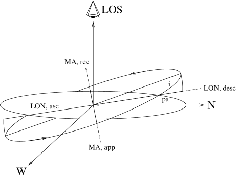
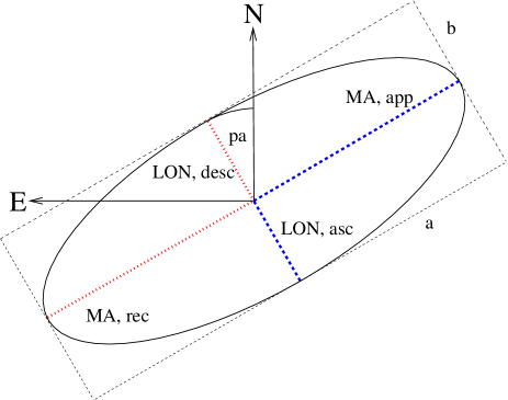
The user specifies the number of rings and for each ring (see also Fig. 1):

• the radius.

• the circular velocity.

• the scale height (for the specification of the vertical density distribution see below).

• the surface brightness.

• the inclination.

• the position angle. Contrary to the usual convention (e.g. GALMOD, ROTCUR), the position angle is defined as the angle between the meridian and the minor axis of each ring from north through east (see Fig. 1). In comparison to GALMOD the TiRiFiC position angle is $90\hbox{${}^{\circ}$}$ larger. TiRiFiC uses the same definition as used by Briggs (1990).

• the right ascension of the central positions of the rings, which is allowed to vary from ring to ring.

• the declination of the central positions of the rings, which is allowed to vary from ring to ring.

• the systemic velocity, which is also allowed to vary from ring to ring.

The user specifies the following global parameters:

• a global isotropic velocity dispersion, which includes the instrumental dispersion. It is clear that such a treatment is not entirely physical, as it is known that the dispersion changes with radius in spiral galaxies and is also not the same in the vertical and horizontal direction of the disk. On the other hand, one has to keep in mind that the tilted-ring model itself is in fact a geometric parametrisation of the galaxy kinematics, which still needs to be interpreted, even if it resembles the true kinematics quite well. The reason to keep a velocity dispersion as a global parameter is to improve the computational speed. It provides the possibility to shift the modelling of the dispersion to a convolution instead of a (time-expensive) Monte-Carlo integration.

• the second global parameter accounts for the vertical distribution of the gas density. The user can chose between a Gaussian, $sech^{2}$, exponential, Lorentzian and a box layer.

• the constant total flux of a single point source (a “cloud”). The number of Monte-Carlo point sources is approximately the total flux of the model divided by this number. When calculating the point sources for a subring, however, the cloud flux is changed by a tiny fraction in order to keep the flux of the subring accurate.

After calculation of a point source model and gridding of the Monte-Carlo point sources onto a model cube, the cube is convolved with a 3D-Gaussian, a product of a 2D (anisotropic) Gaussian in the $x$-$y$-plane, and a 1D Gaussian determined by the global velocity dispersion. The form of the Gaussian in the $x$-$y$-plane is determined by the observing beam of the input cube (the CLEAN beam), which can be redefined by the user.

2.2 $\chi^{2}$ evaluation

The convolution routine implemented in TiRiFiC aims at computational speed. The only possibility to reach the required speed is by an FFT-convolution, for which the FFTW (Frigo & Johnson 2005) library is used. It seems to possess the highest flexibility and quality (in terms of computational speed) of all freely available FFT libraries.

TiRiFiC calculates the $\chi^{2}$ and, along with this, the relative probability of two models. Usually, $\chi^{2}$ is calculated via

$$\begin{aligned} \chi^{2}&=\sum_{k}\frac{(M_{k}-O_{k})^{2}}{\sigma_{k}^{2}}&=\sum_{k}\frac{(M_{k}-O_{k})^{2}}{w_{k}}\end{aligned}\qquad,$$ (1)

where $k$ is an index running over all pixels in the cube, $M$ is the model data cube, $O$ the original, and $\sigma_{k}$ the noise of the original data cube in the $k$th pixel. If the quantisation noise is treated correctly, the weight $w_{k}$ of a pixel should be

$$w(k)=\sigma_{\mathrm{rms}}^{2}+(\sigma^{\mathrm{q}}_{k})^{2}\rm,$$ (2)

where $\sigma_{\mathrm{rms}}$ is the rms noise of the original data cube and $\sigma^{\mathrm{q}}_{k}$ the quantisation noise of the convolved artificial data cube. TiRiFiC is able to calculate $\sigma^{\mathrm{q}}_{k}$ (for a mathematical treatment see Józsa 2006). It is, however, a larger computational effort to do so, and the user might be inclined to modify the goodness-of-fit evaluation. With a “weight parameter” $W$ a weight map is calculated via

$$w_{k}=\frac{\sigma_{\mathrm{rms}}^{2}\cdot W^{2}+(\sigma^{\mathrm{q}}_{k})^{2}}{W^{2}}\qquad.$$ (3)

If $W\rightarrow\infty$, the weight map becomes a constant, $\sigma_{\mathrm{rms}}^{2}$, giving TiRiFiC the possibility to save one convolution. If $W=1$, the noise will be estimated correctly, including the quantisation noise (which can in principle exceed the rms noise of the data cube). The parameter is kept continuous to give the user kind of a weighting scheme at hand. With an increasing weight parameter, the emphasis will be more and more taken away from regions with high quantisation noise (and thus high surface density), towards regions of low surface density.

2.3 $\chi^{2}$ minimisation

With the type of model generation in TiRiFiC, the usual $\chi^{2}$ minimisation algorithms employing partial derivatives of the model function with respect to the fitting parameters like the Levenberg-Marquardt algorithm (Levenberg 1944; Marquardt 1963; Press et al. 1986) are not easily realised, since the analytic form of the fitting function is unknown. The Monte-Carlo method was chosen as a way to produce a model cube because an analytic form of the tilted-ring model does not exist. Furthermore, the model itself, for which a Jacobian would have to be supplied, is the convolved tilted-ring model in three dimensions.

For TiRiFiC the simplest solution without the need for derivatives was implemented first hand. The golden-section search algorithm (Press et al. 1986, Chap. 10.1) is an uneconomic but simple method (see below) to find local $\chi^{2}-$minima in parameter space without the necessity to normalise the $\chi^{2}$ evaluated with TiRiFiC, i.e. for this algorithm the knowledge of the rms noise in the analysed data cube does not play a major role.

A tentatively implemented Metropolis Monte-Carlo-Markov-chain algorithm (Metropolis et al. 1953) proved not to be applicable in tests using real H I data cubes, mainly because a smooth disk as fitted to the data cubes is not close enough to a realistic, clumpy galaxy disk. The Metropolis algorithm requires an ideal parameter-set to be able to reproduce the data perfectly. For more details on the fitting procedure see Józsa (2006, Chap. 2).

Parameter fitting in TiRiFiC is rather flexible. The user can specify single parameters to be fitted, or groups of parameters, which will be fitted at once as one parameter. As an example, the user has the possibility to fit a changing projected centre from ring to ring as is, e.g., expected for a galaxy disk with a bowl-shaped warp. Such bowl-shaped warps result in an asymmetric projected appearance. For rather symmetric galaxies this might not be desirable, because in this case one would desire to keep the number of free parameters low. With TiRiFiC the user has the possibility to fit a single centre for all rings, defining their centres as a group and fitting the value of this group as a whole.

3 Beam smearing and smoothing inherent to velocity fields

The success of a tilted-ring fit to a velocity field depends on how well the velocity field is able to represent the mid-plane recession velocity of the rotating disk. In practice, to derive a velocity field from a data cube one usually tries to determine the peak positions of the velocity profiles (e.g. Swaters 1999, Chap. 3). The simplest way to extract this peak velocity from a noisy velocity profile is to compute the intensity-weighted mean (the first moment, e.g. Rogstad & Shostak 1971; Simon et al. 2003, 2005), while a fit of full Gaussians (e.g. Begemann 1987; Swaters 1999) or half-Gaussians (e.g. García-Ruiz et al. 2002) is considered a better approach. Even more sophisticated methods exist to reliably derive the peak velocities from the line profiles (Gentile et al. 2004). With artificial data cubes, however, one is neither restricted by noise nor by the velocity resolution. Therefore, by producing a noiseless artificial observation with a very high spectral resolution and reading out the peak velocities from the profiles, one gets a velocity field which would ideally be derived from a measured data cube.

It can be shown in a simple experiment that biases will occur in a velocity field-based tilted-ring analysis even when using such an idealised case of a velocity field.

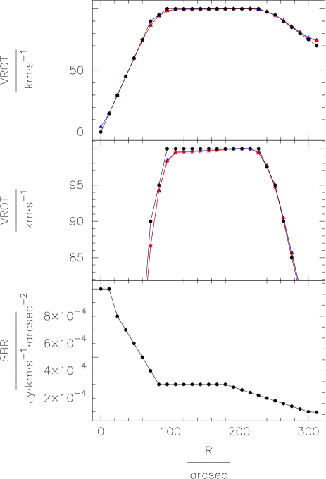
A Gaussian beam with a HPBW of $12\,\arcsec$ and a (total) velocity dispersion of $10\,{\mathrm{km}}\,{\mathrm{s}}^{-1}$ was used to produce with TiRiFiC two low-noise artificial observations of a galaxy with $17.6\cdot 10^{6}$ point sources in a data cube with a spatial pixel separation of $4\arcsec$ (for the parametrisation see Fig. 2, a detailed description can be found in Józsa 2006). The parameters were sampled with a separation of $12\arcsec$. Inclinations of $60\hbox{${}^{\circ}$}$ and $75\hbox{${}^{\circ}$}$ were chosen, and the position angle was kept fixed at all radii.

a)

Figure 2: Testing the extraction of rotation curves from velocity fields. Filled circles and connecting lines (black) show the parametrisation with which two artificial observations have been generated, a velocity field and a data cube (see text). Top panel: rotation curve. Centre panel: blow-up of the rotation curve (same lay-out as above). Bottom panel: H I surface brightness. The inclinations are $60\hbox{${}^{\circ}$}$ (left) and $75\hbox{${}^{\circ}$}$ (right) respectively. Velocity fields were generated as described in the text. Triangles and connecting lines (blue in online version): results from a ROTCUR fit with a free-angle of $0\hbox{${}^{\circ}$}$ and a uniform weighting. Stars and connecting lines (red in online version): results from a ROTCUR fit with a free angle of $30\hbox{${}^{\circ}$}$ and a cosine weighting. Diamonds and connecting lines in the right panel (green in online-version): results from a cut along the galaxy major axis, corrected for inclination. Filled circles and connecting lines (black) also denote the results of a TiRiFiC fit; they are identical to the parametrisations of the artificial observation.

In order to produce a “perfect” velocity field, the cubes were generated with an unrealistic channel separation of $0.26\,{\mathrm{km\,s}}^{-1}$. With these data cubes peak-velocity maps were created. Using these velocity fields, rotation curves were produced using the GIPSY routine ROTCUR, employing two slightly different approaches with an input guess identical to the model parameters, using a sampling of the rings identical to the input model. The results of both fits can be seen in Fig. 2 (see also Teuben 2002).

The fitted rotation velocities are biased following a certain pattern that depends on the shape of the surface brightness profile, which in this test case is falling monotonically. In those regions where the rotation curve is rising, the rotation velocities are underestimated, while in regions where the rotation curve is falling the rotation velocities are overestimated. Hence, the fitted rotation velocity tends to be biased towards regions of higher surface brightness. The reason for this lies in the fact that the measured velocity profile at a certain position of the galaxy is a convolution of the beam with the true intensity distribution. Thus, if the intensity is not constant over the beam area, the resulting “smeared” profile receives more contribution from areas with higher intensity and hence becomes asymmetric, even if it would be symmetric when observed with a pencil-beam. The position of its maximum is dragged towards velocities with a higher associated surface brightness. This effect is cannot be treated in a straightforward manner because it also depends on how velocities change within a beam. It is also visible at radii where both the rotation curve and surface brightness are flat over a large range. This means that “smoothing” affects the rotation curve at all radii. The reason for this lies in the fact that in projection the galaxy becomes fore shortened along the kinematical minor axis. Here, the gradient of the velocity field becomes largest and the observing beam covers the largest range of velocities along the kinematical minor axis. Points in the vicinity of the kinematical minor axis are thus more strongly affected by beam smearing. This is why usually a section of the velocity field is thus not regarded (by specifying a “free-angle”) in a rotation curve analysis and a weighting of data points is applied, while our experiment shows that this treatment does not help much for the analysis of the inner regions, but improves matters in the outer ones. An extreme choice for a free angle would be to only read out the velocities along the major axis of the galaxy and to correct the velocities for the inclination. This is equivalent to an extraction of a rotation curve from a long-slit observation. The results from such a “fit” are shown in the right hand panel of Fig. 2. It can be seen that with such a choice the results get slightly better in the outskirts of the galaxy at the expense of far worse results in its inner parts.

In order to demonstrate how a velocity field analysis is influenced by the a-priori unknown distribution of the H i, we chose a rather high inclination of at least $i=60\hbox{${}^{\circ}$}$ for our artificial observations. Since this covers only one third of all observable galaxies, we emphasise that not necessarily all velocity field analyses are affected by beam smearing. Furthermore, the clumpiness of the distribution of the interstellar medium (ISM) introduces further errors in a tilted-ring analysis, which might well exceed the ones arising from the shown variant of beam smearing.

However, using a velocity field as would be ideally derived in a noiseless observation, we demonstrated how in analysing velocity fields of galaxies with an inclination higher than $i=60\hbox{${}^{\circ}$}$ systematic errors might be introduced by beam smearing. Even if the maximum deviation from the true rotation curve is not very large (about $3.3\,{\mathrm{km\,s}}^{-1}$ for $i=60\hbox{${}^{\circ}$}$ and about $3.9\,{\mathrm{km\,s}}^{-1}$ for $i=75\hbox{${}^{\circ}$}$ in this experiment), this variant of beam smearing can introduce a significant misinterpretation of the measurement, as the resulting rotation curve is systematically biased. Moreover, second order treatments of the kinematics of gaseous disks, like a harmonic analysis, require a precision in that range. An assignment of a (large) statistical error to compensate for beam smearing is thus not a solution. Results from mass decompositions in which (unknown) density profiles are fitted to rotation curves derived from velocity fields are very vulnerable in that respect. The smoothing effect can lead to a preference of rotation curves with a smaller curvature ${\partial^{2}v}/{\partial r^{2}}$.

4 Testing TiRiFiC

4.1 The trivial test

Figure 2 also shows the results of a fit with TiRiFiC to artificial data cubes that are identical to the data cubes used to produce the velocity fields, except for a larger channel width of $2.06\,{\rm km\,s}^{-1}$. As for ROTCUR, the first-guess-parameters were identical to the model parameters and sampled at identical radii. Naturally, TiRiFiC makes a perfect fit and the resulting model is identical to the input model. It is however noticeable that, in principle, with TiRiFiC it is thus possible to produce an artificial observation that can be reproduced by a fitting process over and over. For routines working on the velocity field this is not the case. First, the surface brightness distribution, which is a free extra output of TiRiFiC, has to be inferred using other information (e.g. by fitting a tilted-ring model to the total intensity map). Second, an artificial data cube will always have to be subject to a convolution with an artificial beam, hence introducing beam smearing; therefore, the artificial cube never reproduces a velocity field that fits to the tilted-ring model found by the fitting routine.

4.2 Rotation curve of an edge-on disk

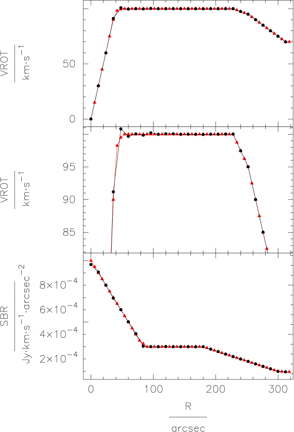
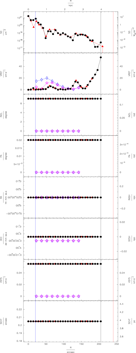
One of the strengths of TiRiFiC is supposed to lie in the ability to perform reliable fits where velocity field methods are bound to fail by definition. This is in particular the case when the line-of-sight crosses the galaxy disk twice or more often. An extreme case of such a situation is encountered when a galaxy is observed (nearly) edge-on, because then the galaxy disk is crossed not only twice but an infinite number of times. We simulated a galaxy observation using the rotation curve and the surface brightness profile shown in Fig. 3, a template cube and an artificial beam as in Sect. 4.1, putting it in an edge-on orientation. The parameters for the artificial observation were sampled in steps of $6\arcsec$. Then, the artificial observation was fitted with TiRiFiC, taking the input model parameters as a first guess, but leaving the rotation velocity, the surface density profile, and the orientational parameters, inclination and position angle as free parameters. In order to prevent a trivial solution, the fitting was performed with a parameter sampling in steps of $12\arcsec$. TiRiFiC reaches a nearly perfect fit, interpolating in the regions where the fit results cannot reproduce the artificial observation by construction (see Fig. 3). Hence, TiRiFiC is in principle able to figure out reliable rotation curves from observations of edge-on galaxies. A slight “beam-smearing” effect takes place at radii where it is not possible to follow the high curvature of the parametrisation of the artificial observation, owing to the fact that in the fitting process the parameters are sampled with half the rate as for the artificial observation.

A caveat is that TiRiFiC assumes a galaxy to be translucent. Observations of edge-on galaxies may suffer significantly from self-absorption and scattering processes at certain wavelengths (e.g. Baes et al. 2003). This has to be taken into account when interpreting TiRiFiC results, especially when fitting to optical spectroscopic data.

Figure 3: Testing rotation curve extraction with TiRiFiC. Triangles and connecting lines (red in online version) show the parametrisation with which a artificial observation of a flat galaxy with $90\hbox{${}^{\circ}$}$ inclination has been generated (edge-on case). Top panel: rotation velocity. Middle panel: rotation velocity, blow-up. Bottom panel: surface brightness. The parametrisation for the artificial observation is twice as dense as for the fit of the artificial observation performed with TiRiFiC. The fitted parameters are represented by dots (black in online version) and connecting lines.

4.3 An edge-on warp

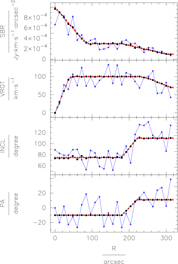
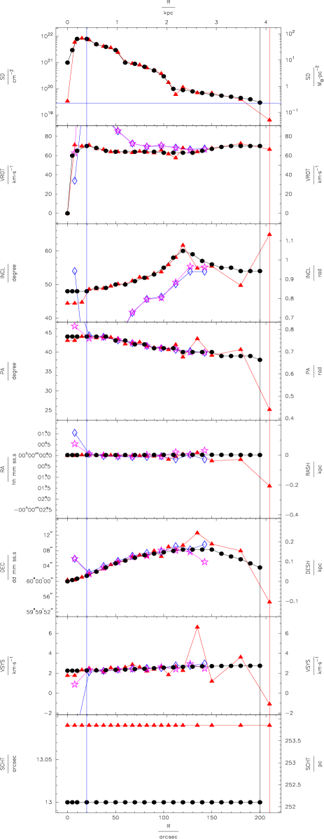
TiRiFiC has been constructed to be able to fit data cubes of observations of warped galaxies, which is one of the main applications of the tilted-ring model. In order to construct a case tailored to put TiRiFiC to the test and for which no appropriate automated software exists yet, a warp in an edge-on galaxy was constructed. This is a situation where it is impossible to construct an unambiguous velocity field, as the line-of-sight crosses the disk several times. Again, the model observation was generated using a template data cube and an artificial beam as described in the previous subsections, sampling the model parameters in steps of $6\arcsec$.

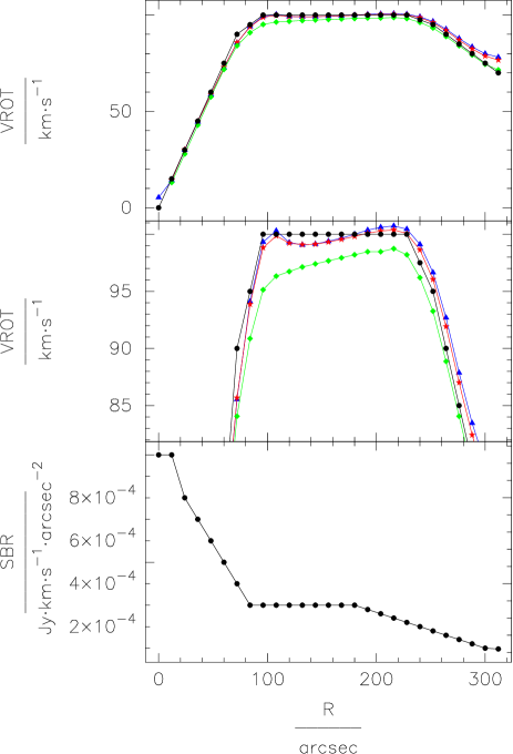
The input parameters to TiRiFiC were chosen to randomly deviate from the input model parameters (see Fig. 4). Again, in fitting the data the model parameters were sampled in steps of $12\arcsec$ in order to prevent the possibility of a trivial solution.

In fitting the data cube, the rotation velocity, surface brightness, inclination and position angle were fitted independently for every single ring; the other parameters were fitted by letting them vary together. An exception was made for the innermost four rings where the orientation parameters were fitted with the constraint to be the same for each ring. A number of $3.5\cdot 10^{6}$ point-sources was chosen for the fitting process, while the artificial observation was created with $17.6\cdot 10^{6}$ point sources.

The result of the fit process (Fig. 4) shows that with TiRiFiC, it is possible to fit to a data cube of an edge-on galaxy with a large warp with a very high accuracy.

Figure 4: Testing tilted-ring fitting with TiRiFiC. Triangles and connecting lines (red in online version) show the parametrisation with which a artificial observation of a heavily warped galaxy has been generated. stars and connecting lines (blue in online version) show the first-guess input to TiRiFiC. The fitted parameters are represented by black filled circles and connecting lines.

4.4 Sensitivity

Since a galactic disk (or any gaseous astronomical object with disk symmetry) becomes fainter with increasing radius, the extent of a tilted-ring analysis is either limited by the observational noise or by the fact that the ring symmetry breaks down. For a conventional velocity field analysis the radial velocities have to be derived from the spectra in the single pixels in a data cube. Hence, the extent of the velocity field and, with this, the maximal radius that can be addressed in a tilted-ring analysis is determined by the pixels where the signal-to-noise ratio significantly exceeds unity. Since with the TiRiFiC approach one fits a global model to the data cube, the number of pixels that determine the parametrisation of a ring is large. Therefore, even if the emission from an object is well below the nominal noise per pixel, one should still be able to derive a reliable parametrisation with TiRiFiC . Provided the object follows a tilted-ring symmetry the detection limit should in theory scale with ${1}/{\sqrt{(}N)}$, where $N$ is the number of pixels with emission in a rotating ring projected onto the 3D data cube.

In order to get an impression of the realistic performance of TiRiFiC when fitting faint structures, we generated a large number of artificial observations of gaseous rings with varying uniform surface brightness and varying surface solid angle. The rings were projected onto a data cube with a size of $512\arcsec\times 512\arcsec$ and a pixel size of $4\arcsec$, 64 channels with a separation of $4.12\,{\rm km}\,{\rm s}^{-1}$ using an observational beam of $12\arcsec\times 14\arcsec$ (Half Power Beam Width), and a global velocity dispersion of $7\,{\rm km}\,{\rm s}^{-1}$. With these specifications, an H i observation with the Westerbork Radio Synthesis Telescope (WSRT) is simulated. In order to add realistic noise to the model, we utilised line-free channels from a $2\times 12\,\rm hrs$ observation with the WSRT having an rms noise level of $3.6\,{\rm mJy}/{\rm beam}$. The rings were chosen to have an inclination of $60\hbox{${}^{\circ}$}$, a rotation velocity of $75\,{\rm km}\,{\rm s}^{-1}$, and a scale height of $2\arcsec$ using a $sech^{2}$-law for the vertical distribution. While the maximal extent of each ring was fixed at $200\arcsec$, the inner radius was varied between $45\arcsec$ and $195\arcsec$, varying linearly the face-on solid angle occupied by the ring, which is roughly proportional to the number of pixels containing emission in the projection of the ring onto the cube.

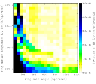
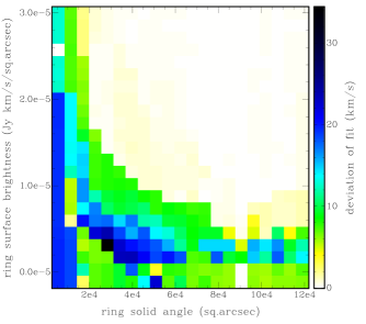
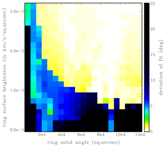
We fitted the artificial observations with rings of the same extent, with an initial guess deviating significantly from the artificial parametrisation (surface brightness $1\cdot 10^{-5}\,{\rm Jy}\,{\rm km}\,{\rm s}^{-1}\,{\rm arcsec}^{-}2$, rotation velocity $65\,{\rm km}\,{\rm s}^{-1}$, inclination and position angle deviating by $10\hbox{${}^{\circ}$}$, all other input parameters identical to the parametrisation of the artificial observation) in a two step process, first fitting all parameters except the surface brightness, then fitting all parameters. In order to distinguish a detection of such a ring from a non-detection we also fitted a data cube containing only noise and no emission. Calculating the differences of the fitted parameters and the parameters used for the artificial observation, one can clearly distinguish between cases where the fit was successful and where it failed (Fig. 5 and Figs. 8 in the online version of this paper).

Figure 5: Testing the sensitivity of TiRiFiC, example. Each pixel represents a fit to a artificial observation (including realistic noise) of an inclined rotating ring with a given solid angle and surface brightness, the lowest row representing a fit to a data cube containing noise only. The pixel values represent the deviation of the fitted position angle from the true position angle of the ring. Clearly distinguishable are regions where the fit succeeded (bright regions) and where it failed (dark regions). Similar plots can be generated for other fitting parameters (see Fig. 8 in the online version of the paper).

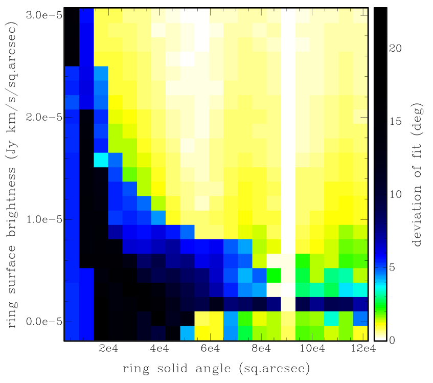
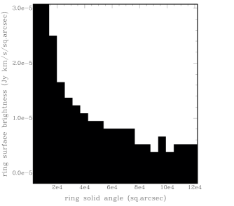
By setting a threshold for the deviations of the parameters, viz. rotation velocity ($4\,{\rm km}\,{\rm s}^{-1}$), surface brightness ($7\cdot 10^{-7}\,{\rm Jy}\,{\rm km}\,{\rm s}^{-1}\,{\rm arcsec}^{-}2$), position angle ($2\hbox{${}^{\circ}$}$), and inclination ($2\hbox{${}^{\circ}$}$), a binary diagram could be constructed in which a detection for combinations of ring surface brightness and ring solid angle was marked (see lower right panel in Fig. 8). Finally, the detection limits as a function of the ring solid angle could be extracted (Fig. 6).

Figure 6: Testing the sensitivity of TiRiFiC. Detection limits as a function of ring-surface solid angle in units of the main beam solid angle ($\Omega_{\rm mb}=202\,{\rm arcsec}^{2}$, see text). The dependence is fairly well fitted by a power law (curved line). The vertical line marks the surface brightness where all pixels in the noiseless data cube lie below the 1-$\sigma_{\rm rms}$ level of the noisy data cube. The right hand axis is scaled such that the surface brightness of a ring is converted to surface column density of an H i observation.

It turned out that while the detection limit determined that way shows a monotonic decrease with increasing ring solid angle, the expected proportionality did not show up. Also when trying to estimate the number of independent data points which the projected ring occupies in the artificial observation we could not establish a simple law that connects the ring solid angle to the detection limits.

However, Fig. 6 clearly shows how the sensitivity in detecting faint symmetric structures in gaseous disks is enhanced using the TiRiFiC approach. With a power law

$$\frac{\sigma_{\rm tir}}{{\rm Jy}\,{\rm km}\,{\rm s}^{-1}\,{\rm arcsec}^{-2}}=9.0\cdot 10^{-4}\cdot\frac{\Omega_{\rm ring}^{-0.82}}{\Omega_{\rm mb}}\qquad,$$ (4)

where $\sigma_{\rm tir}$ is the detection limit and $\Omega_{\rm ring}$ is the ring surface solid angle, and $\Omega_{\rm mb}=202\,{\rm arcsec}^{2}$ the beam solid angle, we achieve a reasonable fit. With this we can estimate the ring solid angle of $141\,\Omega_{\rm mb}$ that is needed to detect a ring that in projection onto the cube has an intensity just below the noise $\sigma_{\rm rms}$ in the data cube ($1.6\cdot 10^{-5}\,{\rm Jy}\,{\rm km}\,{\rm s}^{-1}$ ($\,\hat{\approx}2\cdot 10^{19}\,{\rm atoms}\,{\rm cm}^{-2}$ in an H i observation, horizontal line in Fig. 6). At a radius of $200\arcsec$, this corresponds to a ring width of $24\arcsec$.

A caveat arises from the fact that even when no real emission is present, a fit with TiRiFiC will result in a detection a faint structures in the presence of noise: in a noisy data set a residual offset in surface brightness can be surely found for a specific optimal ring parametrisation even if averaging over many pixels. This can be tested when fitting to a data cube that contains only noise, like it has been done in the experiment discussed here. Figure 7 shows the detected surface brightnesses as a function of ring width when fitting a data cube that contains only noise. The erroneously detected surface brightnesses lie well below the detection limit as quoted in Eq. 4, the detection limit exceedig the erraneously detected surface brightnesses by a factor of a few. However in analysing observations with TiRiFiC, one has to be cautious when accepting a faint structure detected by TiRiFiC as real, since then residual calibration and CLEANing errors become more and more important; in particular cases one should possibly apply additional tests such as the analysis of independent observations.

Figure 7: Resulting surface brightness from a fit of a ring to a cube that contains only noise as a function of ring surface solid angle in units of the beam solid angle ($\Omega_{\rm mb}=202\,{\rm arcsec}^{2}$, see text). Over-plotted is the detection limit determined from fits to faint rings (curved line, see text). The erroneously detected surface brightness lies well below that line.

Compared to e.g. H i observations of nearby spiral galaxies, the size of the test data cube is rather small. Since the surface solid angle of a ring with constant width scales with radius, the detection limits will scale with radius for larger objects. We thus conclude that with TiRiFiC, one is able to detect faint structures well below the noise – provided the observed object shows the symmetry inherent to the tilted-ring model. The detection limits can be estimated as shown above.

4.5 Realistic tests

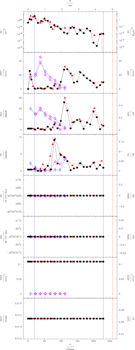
In order to test how TiRiFiC works in practice, we constructed a number of artificial H i observations of galaxies that had to be analysed with TiRiFiC by a (variable) author of this paper, the “observer”. The template cube and the observing beam had the same specifications as given in Sect. 4.4. We performed fits to artificial observations with and without realistic noise added to the data cube as described above, and with varying degrees of symmetry. The observer was informed about the symmetry of the object (like “flat disk” or “constant centre and systemic velocity”), but strictly not about the specific parametrisation of the artificial galaxy disk. We also included cases where all parameters were kept variable and hence a lopsided or a U-shaped galaxy with a possible flare was analysed. Finally, we constructed a case where the cloud flux was drastically enhanced in order to simulate the clumpiness of the gas in the observed object.

All fits were performed following the same pattern. First, the observer estimated the rough geometry of the object from the data cube, in order to then run a first iteration process with TiRiFiC using only a few parameters (fitting a common centre and systemic velocity, a common scale height, a common orientation, and a surface brightness distribution and a rotation curve parametrised by a few data points). After that, the sampling of the parameters was refined and, if necessary, the parameters were fitted independently. It turns out that a fitting process with TiRiFiC needs the personal attention of an observer. In order to achieve a good fit, it is necessary to inspect the results and to correct single data points that are obviously “outliers” in order to restart the fitting process. After a few such iterations (in the range of 2-10) no improvement is achieved and the last fit is the final result.

In order to compare TiRiFiC to methods, where a velocity field is derived and fitted, i.e. a ROTCUR application together with an idealised realistic construction of a velocity field, we additionally generated data cubes with a ten times higher velocity resolution (a channel width of $0.41\,{\rm km}\,{\rm s}^{-1}$) and (if the cube given to the observer contained noise) a ten times lower noise level. The data cubes were flagged where the intensity in the noiseless data cube was below $0.5\sigma_{\rm rms}$. Both a peak intensity and a first moment velocity field was generated from the flagged data cube using the GIPSY routine MOMENTS. This way we simulated the construction of a velocity field as would ideally be derived by an observer (see Sect. 3) using common methods for an extraction of a velocity field. The velocity fields were analysed with ROTCUR, the input guesses either deviating slightly from the optimal guess or being optimal.

A full documentation of all specific fitting results is given in the online version of the paper. Here, we provide a summary.

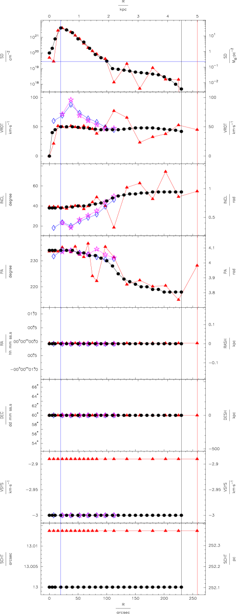
Independent of the specific iteration method preferred by a single observer, TiRiFiC bears reliable results at galactocentric radii greater than 1-1.5 HPBWs (in our example greater than $20\arcsec$). Below that radius, the number of independent data points is too low to allow a fit of the full parameter set. In a statistical sense, TiRiFiC is thus not free from beam smearing but by far less affected than the traditional method: for the bulk of the data points, the ROTCUR results are worse than those of TiRiFiC, and the minimal radius where ROTCUR produces reliable results (under idealised circumstances) lies beyond 4-5 HPBWs of the observing beam.

From Eq. 4 we estimate the detection limit for a ring width of $15\arcsec$ at a radius of $200\arcsec$ to be $2.3\cdot 10^{-5}\,{\rm Jy}\,{\rm km}\,{\rm s}^{-1}$ ($\,\hat{\approx}\,2.9\cdot 10^{19}\,{\rm atoms}\,{\rm cm}^{-2}$ for an H i observation). This value is a conservative upper limit. In most cases the detection limits are significantly lower, especially when the observer could make use of a certain symmetry, e.g. a common centre of all rings.

TiRiFiC fits reliably disks that possess shifting centres and systemic velocities. Hence, with TiRiFiC one is able to fit asymmetric galaxies that maintain the tilted-ring symmetry.

A clumpy H i distribution simulated as described above does not hamper the performance of TiRiFiC. TiRiFiC averages over azimuth, hence a random distribution of a still sizeable number of clouds results in a larger $\chi^{2}$, but not in a different result. We did not simulate the case where the H i distribution is distinctly asymmetric. It is to be suspected that in some cases an m=2 harmonic in the distribution of the tracer material can have an effect on the results.

Above a limit of $25\hbox{${}^{\circ}$}$ in inclination (which is close to (face-on) TiRiFiC disentangles reliably rotation velocity and inclination. In this respect, ROTCUR made a better performance , due to to the fact that our derived velocity fields become very accurate at low inclination. It was shown by Begemann (1987), that for an inclination lower than $60\hbox{${}^{\circ}$}$, inclination and rotation velocity become significantly degenerate in a tilted-ring analysis of the velocity field. For a velocity field analysis with ROTCUR, to derive reliable rotation curves (and with that, a reliable estimate for the inclination) of galaxies with an inclination of less than $40\hbox{${}^{\circ}$}$ it is necessary to apply the method on a velocity field with a statistical error of less than $1\,{rmkm}\,{s}^{-1}$. Such an accuracy is hard to reach using real observational material. In cases with low inclination, the surface density profile determined with TiRiFiC had the smallest errors.

For most parameters a stable solution is found in the first iteration process. The fact that nevertheless a few iterations are needed to reach a final model shows that for some singular parameters the algorithm used for the $\chi^{2}$ minimisation does not perform an effective scann of the parameter space. Then, the user takes the role of stirring up the parameters in order to enable the localisation of the better minimum (for a few data points). The success and the quality of the fits in our tests performed was independent of identity of the observers, who used slightly differing approaches with regards to the fitting parameters and the choice how to approach the best-fit parametrisation from start on. Thus, it seems that the actual way the user shifts singular data points in order to start a next iteration process has no big influence on the quality of results.

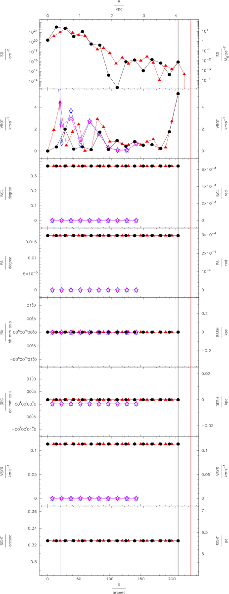
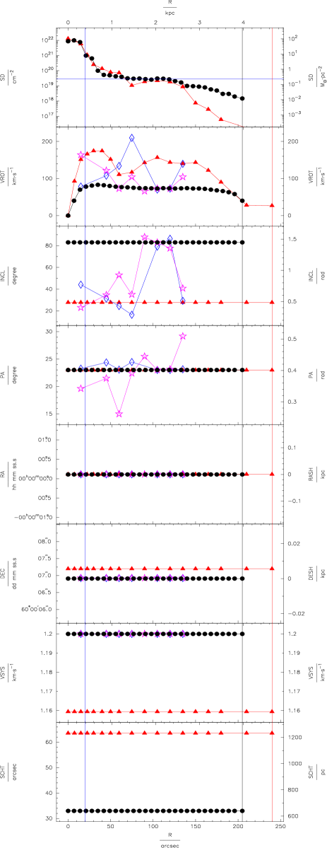
We fail to achieve good results in one particular case with both, TiRiFiC and ROTCUR. In the case of a galaxy with a thick disk (a vertical scale height of $33\arcsec$ in a disk with an H i radius of about $200\arcsec$, see Fig. 10 and Fig. 11 in the online version of the paper), a TiRiFiC fit will converge extremely slowly, since in this case the degeneracy of inclination and rotation velocity is enhanced. This slow convergence then leads to a misinterpretation of the results as being already the final solution. Also ROTCUR fails with extremely large errors, since the kinematical information is smeared out along the kinematical minor axis, making the $\chi^{2}$ minimum in parameter space shallower. In other words, the iso-velocity contours get stretched artificially along the minor axis. In case of TiRiFiC we have the hope to overcome this problem by implementing a more effective minimisation method. The user will in any case be able to detect a thickened disk, and be aware of the problem. We expressively caution, however, against the over-interpretation of rotation curves regardless of the analysis method in the case of galaxies likely to have a thickened disk like it is the case for dIrr galaxies (see e.g. Staveley-Smith et al. 1992; Bottema et al. 1986; Walter & Brinks 1999). Without showing a galactic disk to be thin enough, these rotation curves are extremely unreliable.

4.6 Solid-body rotation

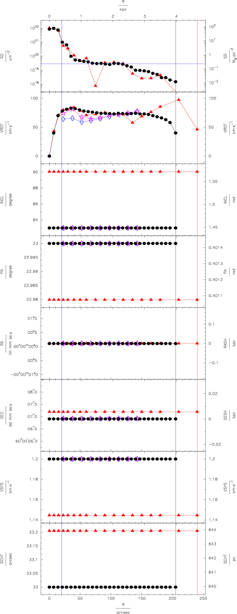
Another problem occurring when extracting rotation curves using velocity fields occurs in the case of a solid-body rotation, as can be found again in dIrr galaxies (e.g. Walter & Brinks 1999). In that case, rotation velocity and inclination are completely degenerate. Since with TiRiFiC one fits not only the kinematics but also the radial surface brightness profile, this degeneracy is broken, provided the gas distribution is symmetric enough and shows a radial gradient, as we can show in a further experiment (last viewgraph in the online version of the paper) that we performed with the same specifications for the artificial observation as given in Sect. 4.5 using a noiseless data cube. TiRiFiC fits very reliably a flat disk with solid-body rotation.

4.7 TiRiFiC performance

TiRiFiC is slow. Nearly 160 hours computation time needed to perform the fit described in Sect. 4.3, working with an AMD Athlon XP 2400+ CPU, can serve as an orientation. In practice, however, the user has the possibility to reduce the computing time considerably. In a first iteration process, the size of the data cube can be reduced by binning data points. The model can be ported easily from a low-resolution data cube to a high-resolution data cube, since the model parameters are independent of the specifications of the data cube, unless the reference coordinate system (the epoch and the velocity definition) changes. Assumptions about symmetries can be made in order to reduce the number of parameters. E.g., if a disk is not warped, all position angles and inclinations can be fitted as one single parameter. A-priori known parameters like a surface brightness profile can be excluded from the fitting process.

Up to now, we concentrated on an implementation of a working version of the software in order to demonstrate its applicability. Future development, however, will include a parallelisation of the code in order to make the use of computer clusters possible. Furthermore, the possibilities to use more sensible fitting procedures will be explored. With this we certainly expect a jump in the computing performance of TiRiFiC.

5 Results and discussion

We introduce TiRiFiC as a program that fits a tilted-ring model directly to spectroscopic data cubes and we provide a number of tests of the program. We show that the TiRiFiC tilted-ring model has a high flexibility and even allows modelling of galaxy disks that are asymmetric in projection. We are able to show that TiRiFiC is not affected by the drawbacks of methods that work on velocity fields. For galaxies with an inclination above $60\hbox{${}^{\circ}$}$, we show that velocity fields are affected by systematics that depend on a-priori unknown factors, such as the surface density distribution. While the deviations of a rotation curve from the true one derived with fits to the velocity field are small, they occur in a systematic manner, possibly biasing the results of a rotation curve analysis. Using a direct fit to the data cube, TiRiFiC reduces these systematics significantly, delivering the unknown surface density profile as an extra. A finite observing beam affects the reliability of the TiRiFiC results at the smallest radii in a statistical sense, since the number of fit parameters becomes too large in comparison to the number of independent data points. In general, TiRiFiC delivers more reliable results than a fit to the velocity field.

The biggest advantage of TiRiFiC lies in its applicability to edge-on and warped galaxies. Several tests show that TiRiFiC is able to reach a best-fit model that comes very close to artificial input models having a large edge-on warp.

Since the approach of TiRiFiC is to fit a global model to the data cube, a detection and quantification of a faint outer disk is possible, even if the bulk of the emission of that disk is fainter than the rms noise of the data cube, provided the outer disk follows the tilted-ring symmetry.

TiRiFiC fails to disentangle inclination and rotation velocity below a disk inclination of $25\hbox{${}^{\circ}$}$ (i.e. close to face-on). In that case, to estimate a more reliable rotation curve, a velocity field approach is to be preferred.

The determination of rotation curves for galaxies with very thick disks like dIrr galaxies is unreliable, regardless of the fitting method, since the degeneracy of inclination and rotation velocity is significantly enhanced. Since the surface-brightness distribution is also fitted by TiRiFiC, it is nevertheless possible with this approach to derive reliable rotation curves in the case of solid-body rotation that occurs predominantly in dIrr galaxies.

The major current drawback of TiRiFiC is its slowness. Performing a single fit when using a conventional PC takes a long time. Hence, TiRiFiC is not (yet) usable to perform many fits in a short time unless a certain amount of computational power can be employed.

We present a series of practical tests in the course of which an “observer” had to parametrise an unknown galactic disk with TiRiFiC, and we are able to show that such a parametrisation is reliable even when analysing data cubes with realistic noise. The success in the limits stated above is independent of the specific approach of the observer. It is of course the application to real observational data as will be presented in subsequent papers of this series that will show how useful TiRiFiC is in gaining new insights in the kinematic structure of rotating disks, especially galaxy disks. TiRiFiC can be considered as the most straightforward realisation of a tilted-ring fitting method, since with its approach one does not require any careful analysis of the single spectra in a data cube in order to extract a velocity field. Hence, if TiRiFiC fails to produce a model data cube that fits to an observation of a galactic disk, the implication is that its kinematics cannot be represented by a tilted-ring model. The development of fitting routines similar to TiRiFiC is a good step towards improving analysis methods of observational data containing kinematical information, as will be demonstrated in the consecutive papers of this series. As secondary kinematical features (and their influence on the analysis) not compliant with the tilted-ring model have received more and more attention in the recent literature, e.g. by applying harmonical analyses, the aim must be to extend the analysis tools in order to put theory of galactic structure formation that includes non-circular motions to the test. This work is already in progress.

6 TiRiFiC sensitivity: additional plots

Figure 8: Testing the sensitivity of TiRiFiC. Each pixel represents a fit to a artificial observation (including realistic noise) of an inclined rotating ring with a given solid angle and surface brightness, the lowest row representing a fit to a data cube containing noise only. The pixel values represent the deviation of the fitted surface brightness (upper left panel), the rotation velocity (upper right panel), and the inclination (lower left panel) from the known true values. Clearly distinguishable are the regions where the fit succeeded (bright regions) and where the fit failed (dark regions). By setting a threshold a binary diagram can be generated (lower right panel), from which the detection limits in dependence of the ring surface solid angle can be estimated (Fig. 6).

7 Testing TiRiFiC: individual tests

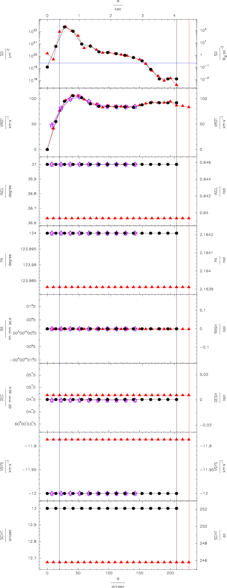
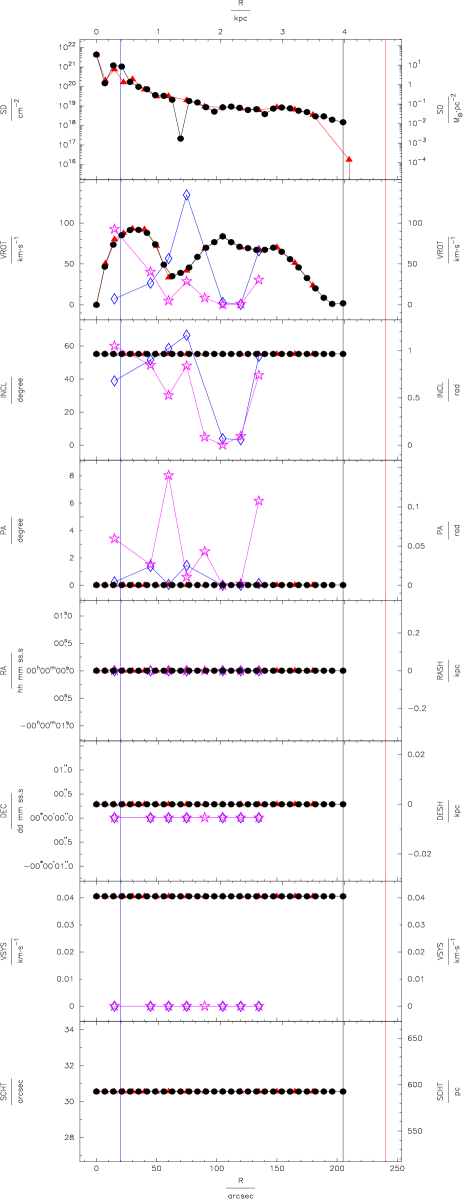
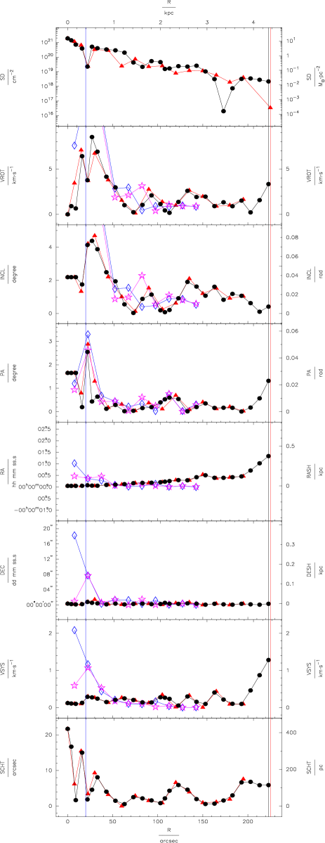
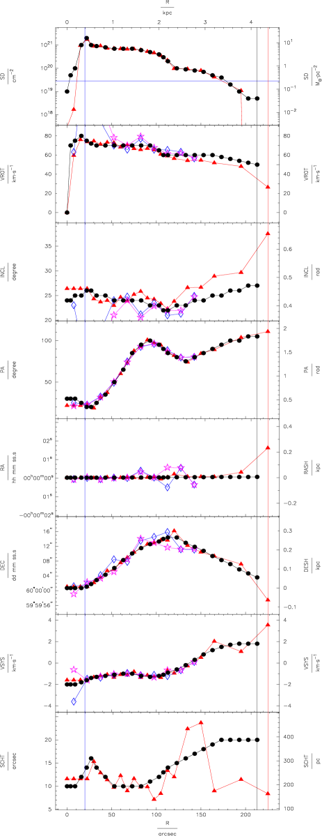
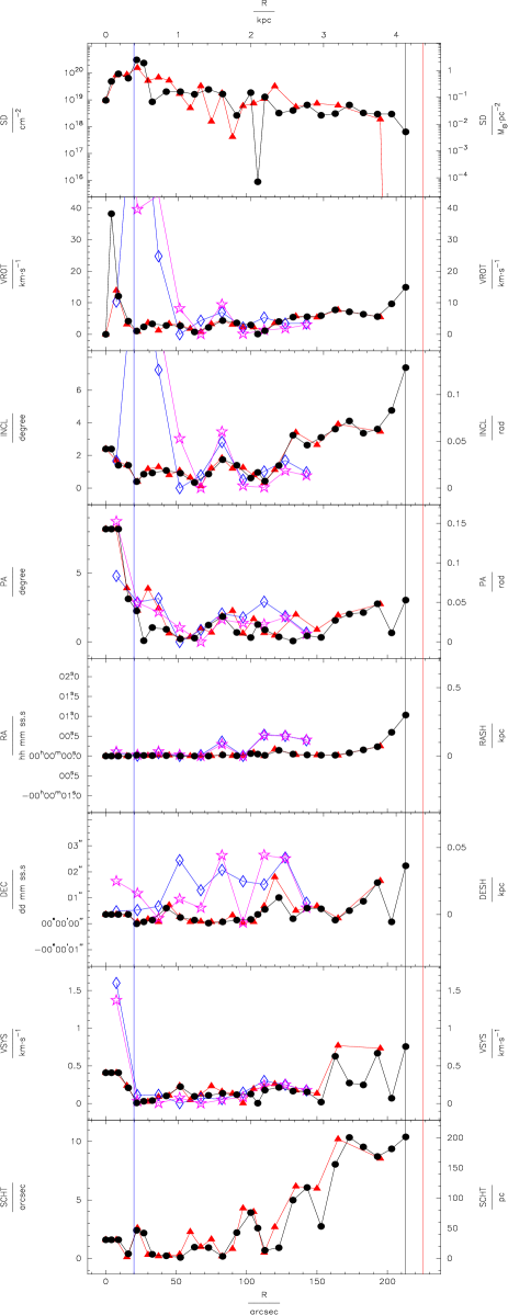
TiRiFiC was tested by constructing a number of artificial observations of a number of H i disks of a galaxy at a distance of $4\,\rm Mpc$. Here we show the results of the fits, which were performed by an “observer” using TiRiFiC. In addition, we present the results derived with ROTCUR on idealised velocity fields, which were extracted from a artificial observation of the same disk with ten times lower noise and ten times higher velocity resolution. ROTCUR was run on a peak-velocity field and a first-moment velocity field, the input guesses reported in the captions. The fit was performed using a free angle of $45\hbox{${}^{\circ}$}$, fixing the expansion velocity of the rings to $0\,{\rm km}\,{\rm s}^{-1}$. For each test we provide a plot (left) containing the parametrisation of the artificial disk (black dots and connecting black lines), the results of the TiRiFiC fit (red triangles and connecting lines), and the results of both ROTCUR fits (blue diamonds and connecting lines: fit to first-moment velocity field, stars in magenta and connecting lines: fit to the peak velocity field). From top to bottom the panels contain: SD: H i face-on column density and surface density in ${\rm atoms}\,{\rm cm}^{-2}$ and ${\rm M}_{\odot}\,{\rm pc}^{-2}$, respectively. VROT: rotation velocity in ${\rm km}\,{\rm s}^{-1}$. INCL: inclination in degrees and radians, respectively. PA: position angle in degrees and radians. RA: the right ascension of the central position in hh:mm:ss. RASH: the projected shift in right ascension in $\rm kpc$ with respect to the centre of ring 1. DEC: the declination of the central position in dd:mm:ss. DESH: the projected shift in declination in $\rm kpc$ with respect to the centre of ring 1. VSYS: the systemic velocity in ${\rm km}\,{\rm s}^{-1}$. SCHT: the scale height in arcseconds and $\rm pc$, respectively. The black vertical line marks the end of the artificial disk, while the red vertical line marks the end of the disk modelled by the observer. The blue vertical line marks a radius of 1.5 HPBWs, beyond which TiRiFiC produces reliable results in nearly all cases. The blue horizontal line marks the detection limit for a ring of $15\arcsec$ width at a radius of $200\arcsec$ as derived in Sect. 4.4. The right-hand graph shows the deviations of the TiRiFiC fits from the model parametrisations. Black dots and lines represent the deviation of the black dots (the true parametrisation of the artificial galaxy) in the left viewgraph from the red lines (the parametrisation fitted with TiRiFiC) in the left panel, in red the deviation of the red triangles (the parametrisation fitted with TiRiFiC) in the left panel from the black lines (the true parametrisation of the artificial galaxy) in the left panel. Blue diamonds show the deviation of the ROTCUR fit to the first-moment velocity field from the parametrisation of the artificial galaxy, stars in magenta show the deviation of the ROTCUR fit to the peak-velocity field from the parametrisation of the artificial galaxy. The vertical lines in the right-hand plot have the same meaning as in the left-hand plot.

We analysed the quality of the TiRiFiC fits by means of statistics. To this end, we extracted the deviations of the fits from the parametrisation of the artificial galaxy and built the mean and rms, and calculated the maximal error. The tables contain:
(1) The quantity listed. $\overline{\Delta}$: mean of deviations. $\sqrt{\overline{\Delta^{2}}}$: rms of deviations. $\Delta_{\rm max}$: Maximum deviation in the range described by (2).
(2) The range in which the deviations were determined. all: taking all data points into account. 70%: taking the 70% lowest deviations into account. $n-\sigma$: taking those data points into account where the expected surface brightness is below the $n-\sigma$- level of the artificial observation. The $1-\sigma$ level is determined by the face-on column density of a ring constructed as described in Sect. 4.4, which in projection onto a data cube contains no emission above the $1-\sigma_{\rm rms}$ level in the noisy data cube ($\sigma=2\cdot 10^{19}\,{\rm atoms}\,{\rm cm}^{-2}$). excs: only for the surface column density: deviations where the expected surface column density is 0, i.e. where the artificial disk has already ended.
(3) Method to determine the quantities. tir: use of TiRiFiC. m1: use of ROTCUR, fitting to the first-moment velocity field. pk: use of ROTCUR, fitting to the peak-velocity field.
(4) Error in face-on H i column density ($10^{18}\,{\rm atoms}\,{\rm cm}^{-2}$).
(5) Ratio of error in face-on H i column density and expected face-on H i column density.
(6) Error in rotation velocity (${\rm km}\,{\rm s}^{-1}$).
(7) Error in inclination ( ^∘).
(8) Error in position angle ( ^∘).
(9) Error in right ascension of ring centre ($\,\arcsec$).
(10) Error in declination of ring centre ($\,\arcsec$).
(11) Error in systemic velocity (${\rm km}\,{\rm s}^{-1}$).
(12) Error in scale height ($\,\arcsec$).

Figure 9: Test 1: Flat disk with constant scale height without noise. The orientation parameters, centre, systemic velocity and scale height were fitted ”as one” with TiRiFiC. ROTCUR: input model with optimal guesses. Only the rotation velocity was fitted. For symbol- and colour coding see the introduction to this section.

Table 1: Test 1: Flat disk with constant scale height without noise. The orientation parameters, centre, systemic velocity and scale height were fitted ”as one” with TiRiFiC. Deviation in global dispersion: 0.01 ${\rm km}\,{\rm s}^{-1}$. ROTCUR: input model with optimal guesses. Only the rotation velocity was fitted.

Quantity	Range	method	$N_{{H\textsc{i}}}$	$\frac{N_{{H\textsc{i}}}}{N_{{H\textsc{i}}},exp}$	$v_{\rm rot}$	$i$	$pa$	${\rm RA}$	${\rm DEC}$	$v_{\rm sys}$	$z_{0}$
(1)	(2)	(3)	(4)	(5)	(6)	(7)	(8)	(9)	(10)	(11)	(12)
$\overline{\Delta}$	all	tir	257.32	0.710	1.4	0.4	0.0	0.2	0.2	0.1	0.3
$\sqrt{\overline{\Delta^{2}}}$	all	tir	625.61	2.610	2.0	0.4	0.0	0.2	0.2	0.1	0.3
$\Delta_{\rm max}$	all	tir	2629.47	12.176	5.3	0.4	0.0	0.2	0.2	0.1	0.3
$\overline{\Delta}$	70%	tir	4.00	0.058	0.6	0.4	0.0	0.2	0.2	0.1	0.3
$\sqrt{\overline{\Delta^{2}}}$	70%	tir	8.17	0.071	0.8	0.4	0.0	0.2	0.2	0.1	0.3
$\Delta_{\rm max}$	70%	tir	25.31	0.117	1.8	0.4	0.0	0.2	0.2	0.1	0.3
$\overline{\Delta}$	hi	tir	353.39	0.088	1.1	0.4	0.0	0.2	0.2	0.1	0.3
$\sqrt{\overline{\Delta^{2}}}$	hi	tir	793.24	0.149	1.4	0.4	0.0	0.2	0.2	0.1	0.3
$\Delta_{\rm max}$	hi	tir	2629.47	0.481	2.9	0.4	0.0	0.2	0.2	0.1	0.3
$\overline{\Delta}$	$8-\sigma$	tir	0.99	0.140	1.3	0.4	0.0	0.2	0.2	0.1	0.3
$\sqrt{\overline{\Delta^{2}}}$	$8-\sigma$	tir	1.43	0.242	2.0	0.4	0.0	0.2	0.2	0.1	0.3
$\Delta_{\rm max}$	$8-\sigma$	tir	3.35	0.678	5.3	0.4	0.0	0.2	0.2	0.1	0.3
$\overline{\Delta}$	$2-\sigma$	tir	0.72	0.221	1.7	0.4	0.0	0.2	0.2	0.1	0.3
$\sqrt{\overline{\Delta^{2}}}$	$2-\sigma$	tir	1.27	0.312	2.5	0.4	0.0	0.2	0.2	0.1	0.3
$\Delta_{\rm max}$	$2-\sigma$	tir	3.35	0.678	5.3	0.4	0.0	0.2	0.2	0.1	0.3
$\overline{\Delta}$	$0.5-\sigma$	tir	0.34	0.241	1.9	0.4	0.0	0.2	0.2	0.1	0.3
$\sqrt{\overline{\Delta^{2}}}$	$0.5-\sigma$	tir	0.50	0.337	2.7	0.4	0.0	0.2	0.2	0.1	0.3
$\Delta_{\rm max}$	$0.5-\sigma$	tir	0.95	0.678	5.3	0.4	0.0	0.2	0.2	0.1	0.3
$\overline{\Delta}$	excs	tir	0.03
$\sqrt{\overline{\Delta^{2}}}$	excs	tir	0.04
$\Delta_{\rm max}$	excs	tir	0.05
$\overline{\Delta}$	all	pk			3.1	0.0	0.0	0.0	0.0	0.0
$\sqrt{\overline{\Delta^{2}}}$	all	pk			6.2	0.0	0.0	0.0	0.0	0.0
$\Delta_{\rm max}$	all	pk			0.0	0.0	0.0	0.0	0.0	0.0
$\overline{\Delta}$	70%	pk			0.9	0.0	0.0	0.0	0.0	0.0
$\sqrt{\overline{\Delta^{2}}}$	70%	pk			1.2	0.0	0.0	0.0	0.0	0.0
$\Delta_{\rm max}$	70%	pk			2.4	0.0	0.0	0.0	0.0	0.0
$\overline{\Delta}$	hi	pk			1.3	0.0	0.0	0.0	0.0	0.0
$\sqrt{\overline{\Delta^{2}}}$	hi	pk			1.7	0.0	0.0	0.0	0.0	0.0
$\Delta_{\rm max}$	hi	pk			3.0	0.0	0.0	0.0	0.0	0.0
$\overline{\Delta}$	all	m1			2.7	0.0	0.0	0.0	0.0	0.0
$\sqrt{\overline{\Delta^{2}}}$	all	m1			5.5	0.0	0.0	0.0	0.0	0.0
$\Delta_{\rm max}$	all	m1			0.0	0.0	0.0	0.0	0.0	0.0
$\overline{\Delta}$	70%	m1			0.6	0.0	0.0	0.0	0.0	0.0
$\sqrt{\overline{\Delta^{2}}}$	70%	m1			0.8	0.0	0.0	0.0	0.0	0.0
$\Delta_{\rm max}$	70%	m1			1.6	0.0	0.0	0.0	0.0	0.0
$\overline{\Delta}$	hi	m1			1.2	0.0	0.0	0.0	0.0	0.0
$\sqrt{\overline{\Delta^{2}}}$	hi	m1			1.7	0.0	0.0	0.0	0.0	0.0
$\Delta_{\rm max}$	hi	m1			3.7	0.0	0.0	0.0	0.0	0.0

Figure 10: Test 2: Flat disk with constant large scale height; noise added to the cube. Orientation parameters, centre, systemic velocity and scale height fitted ”as one” with TiRiFiC. In a first attempt the observer failed to achieve a good fit. The large scale height enhances drastically the ambiguity of inclination and rotation velocity. ROTCUR: input model with optimal guesses. Only the rotation velocity and the orientation parameters were fitted. For symbol- and colour coding see the introduction to this section.

Table 2: Test 2: Flat disk with constant large scale height; noise added to the cube. Orientation parameters, centre, systemic velocity and scale height fitted ”as one” with TiRiFiC. In a first attempt the observer failed to achieve a good fit. The large scale height enhances drastically the ambiguity of inclination and rotation velocity. Deviation in global dispersion: 0.57 ${\rm km}\,{\rm s}^{-1}$. ROTCUR: input model with optimal guesses. Only the rotation velocity and the orientation parameters were fitted.

Quantity	Range	method	$N_{{H\textsc{i}}}$	$\frac{N_{{H\textsc{i}}}}{N_{{H\textsc{i}}},exp}$	$v_{\rm rot}$	$i$	$pa$	${\rm RA}$	${\rm DEC}$	$v_{\rm sys}$	$z_{0}$
(1)	(2)	(3)	(4)	(5)	(6)	(7)	(8)	(9)	(10)	(11)	(12)
$\overline{\Delta}$	all	tir	327.61	0.536	61.6	55.2	0.0	0.1	0.3	0.0	30.6
$\sqrt{\overline{\Delta^{2}}}$	all	tir	1038.29	0.624	66.7	55.2	0.0	0.1	0.3	0.0	30.6
$\Delta_{\rm max}$	all	tir	4323.01	1.052	93.2	55.2	0.0	0.1	0.3	0.0	30.6
$\overline{\Delta}$	70%	tir	11.14	0.353	49.9	55.2	0.0	0.1	0.3	0.0	30.6
$\sqrt{\overline{\Delta^{2}}}$	70%	tir	15.28	0.403	54.7	55.2	0.0	0.1	0.3	0.0	30.6
$\Delta_{\rm max}$	70%	tir	32.42	0.646	72.0	55.2	0.0	0.1	0.3	0.0	30.6
$\overline{\Delta}$	hi	tir	80.80	0.579	72.0	55.2	0.0	0.1	0.3	0.0	30.6
$\sqrt{\overline{\Delta^{2}}}$	hi	tir	114.15	0.642	75.6	55.2	0.0	0.1	0.3	0.0	30.6
$\Delta_{\rm max}$	hi	tir	237.01	1.052	93.2	55.2	0.0	0.1	0.3	0.0	30.6
$\overline{\Delta}$	$8-\sigma$	tir	15.72	0.662	61.3	55.2	0.0	0.1	0.3	0.0	30.6
$\sqrt{\overline{\Delta^{2}}}$	$8-\sigma$	tir	24.48	0.721	64.6	55.2	0.0	0.1	0.3	0.0	30.6
$\Delta_{\rm max}$	$8-\sigma$	tir	70.63	1.052	92.4	55.2	0.0	0.1	0.3	0.0	30.6
$\overline{\Delta}$	$2-\sigma$	tir	7.01	0.601	59.6	55.2	0.0	0.1	0.3	0.0	30.6
$\sqrt{\overline{\Delta^{2}}}$	$2-\sigma$	tir	8.80	0.669	62.3	55.2	0.0	0.1	0.3	0.0	30.6
$\Delta_{\rm max}$	$2-\sigma$	tir	19.74	0.983	83.7	55.2	0.0	0.1	0.3	0.0	30.6
$\overline{\Delta}$	$0.5-\sigma$	tir	3.75	0.953	48.5	55.2	0.0	0.1	0.3	0.0	30.6
$\sqrt{\overline{\Delta^{2}}}$	$0.5-\sigma$	tir	5.10	0.954	52.2	55.2	0.0	0.1	0.3	0.0	30.6
$\Delta_{\rm max}$	$0.5-\sigma$	tir	8.64	0.983	70.6	55.2	0.0	0.1	0.3	0.0	30.6
$\overline{\Delta}$	excs	tir	0.01
$\sqrt{\overline{\Delta^{2}}}$	excs	tir	0.01
$\Delta_{\rm max}$	excs	tir	0.02
$\overline{\Delta}$	all	pk			25.7	29.9	2.8	0.0	0.0	0.0
$\sqrt{\overline{\Delta^{2}}}$	all	pk			38.8	37.1	3.9	0.0	0.0	0.0
$\Delta_{\rm max}$	all	pk			92.6	60.0	8.0	0.0	0.0	0.0
$\overline{\Delta}$	70%	pk			8.5	16.6	0.9	0.0	0.0	0.0
$\sqrt{\overline{\Delta^{2}}}$	70%	pk			13.5	23.5	1.3	0.0	0.0	0.0
$\Delta_{\rm max}$	70%	pk			28.6	42.3	2.5	0.0	0.0	0.0
$\overline{\Delta}$	hi	pk			18.4	31.7	2.5	0.0	0.0	0.0
$\sqrt{\overline{\Delta^{2}}}$	hi	pk			24.8	37.3	4.1	0.0	0.0	0.0
$\Delta_{\rm max}$	hi	pk			40.2	48.4	8.0	0.0	0.0	0.0
$\overline{\Delta}$	all	m1			42.0	39.5	0.5	0.0	0.0	0.0
$\sqrt{\overline{\Delta^{2}}}$	all	m1			61.5	46.2	0.8	0.0	0.0	0.0
$\Delta_{\rm max}$	all	m1			134.5	66.6	1.4	0.0	0.0	0.0
$\overline{\Delta}$	70%	m1			9.3	24.5	0.1	0.0	0.0	0.0
$\sqrt{\overline{\Delta^{2}}}$	70%	m1			13.8	32.4	0.1	0.0	0.0	0.0
$\Delta_{\rm max}$	70%	m1			26.5	51.6	0.1	0.0	0.0	0.0
$\overline{\Delta}$	hi	m1			55.1	45.2	0.7	0.0	0.0	0.0
$\sqrt{\overline{\Delta^{2}}}$	hi	m1			74.2	51.3	1.0	0.0	0.0	0.0
$\Delta_{\rm max}$	hi	m1			134.5	66.6	1.4	0.0	0.0	0.0

Figure 11: Test 2, after revision: same as 2, but this time started near to the correct result. The observer achieved a reasonable result, while TiRiFiC approached the $\chi^{2}$ minimum in parameter space very slowly. It is to be hoped that this problem will vanish after the implementation of a more effective $\chi^{2}$ minimiser. ROTCUR: input model with optimal guesses. Only the rotation velocity was fitted. For symbol- and colour coding see the introduction to this section.

Table 3: Test 2, revised: same as 2, but this time started tear to the correct result. The observer achieved a reasonable result, while TiRiFiC approached the $\chi^{2}$ minimum in parameter space very slowly. It is to be hoped that this problem will vanish after the implementation of a more effective $\chi^{2}$ minimiser. Deviation in global dispersion: 0.39 ${\rm km}\,{\rm s}^{-1}$. ROTCUR: input model with optimal guesses. Only the rotation velocity was fitted.

Quantity	Range	method	$N_{{H\textsc{i}}}$	$\frac{N_{{H\textsc{i}}}}{N_{{H\textsc{i}}},exp}$	$v_{\rm rot}$	$i$	$pa$	${\rm RA}$	${\rm DEC}$	$v_{\rm sys}$	$z_{0}$
(1)	(2)	(3)	(4)	(5)	(6)	(7)	(8)	(9)	(10)	(11)	(12)
$\overline{\Delta}$	all	tir	160.22	0.386	4.0	7.1	0.0	0.1	0.3	0.1	0.2
$\sqrt{\overline{\Delta^{2}}}$	all	tir	435.21	0.483	6.7	7.1	0.0	0.1	0.3	0.1	0.2
$\Delta_{\rm max}$	all	tir	1752.18	0.975	18.8	7.1	0.0	0.1	0.3	0.1	0.2
$\overline{\Delta}$	70%	tir	8.43	0.217	1.1	7.1	0.0	0.1	0.3	0.1	0.2
$\sqrt{\overline{\Delta^{2}}}$	70%	tir	13.12	0.271	1.4	7.1	0.0	0.1	0.3	0.1	0.2
$\Delta_{\rm max}$	70%	tir	30.33	0.608	2.9	7.1	0.0	0.1	0.3	0.1	0.2
$\overline{\Delta}$	hi	tir	87.62	0.485	2.2	7.1	0.0	0.1	0.3	0.1	0.2
$\sqrt{\overline{\Delta^{2}}}$	hi	tir	147.64	0.573	2.9	7.1	0.0	0.1	0.3	0.1	0.2
$\Delta_{\rm max}$	hi	tir	361.90	0.975	6.6	7.1	0.0	0.1	0.3	0.1	0.2
$\overline{\Delta}$	$8-\sigma$	tir	11.54	0.478	5.5	7.1	0.0	0.1	0.3	0.1	0.2
$\sqrt{\overline{\Delta^{2}}}$	$8-\sigma$	tir	18.51	0.561	8.1	7.1	0.0	0.1	0.3	0.1	0.2
$\Delta_{\rm max}$	$8-\sigma$	tir	48.88	0.975	18.8	7.1	0.0	0.1	0.3	0.1	0.2
$\overline{\Delta}$	$2-\sigma$	tir	6.70	0.464	6.3	7.1	0.0	0.1	0.3	0.1	0.2
$\sqrt{\overline{\Delta^{2}}}$	$2-\sigma$	tir	10.64	0.546	9.1	7.1	0.0	0.1	0.3	0.1	0.2
$\Delta_{\rm max}$	$2-\sigma$	tir	29.82	0.975	18.8	7.1	0.0	0.1	0.3	0.1	0.2
$\overline{\Delta}$	$0.5-\sigma$	tir	2.40	0.523	9.5	7.1	0.0	0.1	0.3	0.1	0.2
$\sqrt{\overline{\Delta^{2}}}$	$0.5-\sigma$	tir	3.58	0.562	11.6	7.1	0.0	0.1	0.3	0.1	0.2
$\Delta_{\rm max}$	$0.5-\sigma$	tir	6.77	0.720	18.8	7.1	0.0	0.1	0.3	0.1	0.2
$\overline{\Delta}$	excs	tir	0.09
$\sqrt{\overline{\Delta^{2}}}$	excs	tir	0.13
$\Delta_{\rm max}$	excs	tir	0.18
$\overline{\Delta}$	all	pk			5.2	0.0	0.0	0.0	0.0	0.0
$\sqrt{\overline{\Delta^{2}}}$	all	pk			6.6	0.0	0.0	0.0	0.0	0.0
$\Delta_{\rm max}$	all	pk			0.0	0.0	0.0	0.0	0.0	0.0
$\overline{\Delta}$	70%	pk			2.6	0.0	0.0	0.0	0.0	0.0
$\sqrt{\overline{\Delta^{2}}}$	70%	pk			2.9	0.0	0.0	0.0	0.0	0.0
$\Delta_{\rm max}$	70%	pk			4.7	0.0	0.0	0.0	0.0	0.0
$\overline{\Delta}$	hi	pk			6.6	0.0	0.0	0.0	0.0	0.0
$\sqrt{\overline{\Delta^{2}}}$	hi	pk			7.8	0.0	0.0	0.0	0.0	0.0
$\Delta_{\rm max}$	hi	pk			12.0	0.0	0.0	0.0	0.0	0.0
$\overline{\Delta}$	all	m1			9.7	0.0	0.0	0.0	0.0	0.0
$\sqrt{\overline{\Delta^{2}}}$	all	m1			11.9	0.0	0.0	0.0	0.0	0.0
$\Delta_{\rm max}$	all	m1			0.0	0.0	0.0	0.0	0.0	0.0
$\overline{\Delta}$	70%	m1			5.9	0.0	0.0	0.0	0.0	0.0
$\sqrt{\overline{\Delta^{2}}}$	70%	m1			7.6	0.0	0.0	0.0	0.0	0.0
$\Delta_{\rm max}$	70%	m1			14.7	0.0	0.0	0.0	0.0	0.0
$\overline{\Delta}$	hi	m1			13.0	0.0	0.0	0.0	0.0	0.0
$\sqrt{\overline{\Delta^{2}}}$	hi	m1			14.3	0.0	0.0	0.0	0.0	0.0
$\Delta_{\rm max}$	hi	m1			20.1	0.0	0.0	0.0	0.0	0.0

Figure 12: Test 3: symmetric warp without central shift and without shift in systemic velocity. Noise was added to the data cube. ROTCUR: input model with optimal guesses. Only the rotation velocity and the orientation parameters were fitted. For symbol- and colour coding see the introduction to this section.

Table 4: Test 3: symmetric warp without central shift and without shift in systemic velocity. Noise was added to the data cube. Deviation in global dispersion: 0.03 ${\rm km}\,{\rm s}^{-1}$. ROTCUR: input model with optimal guesses. Only the rotation velocity and the orientation parameters were fitted.

Quantity	Range	method	$N_{{H\textsc{i}}}$	$\frac{N_{{H\textsc{i}}}}{N_{{H\textsc{i}}},exp}$	$v_{\rm rot}$	$i$	$pa$	${\rm RA}$	${\rm DEC}$	$v_{\rm sys}$	$z_{0}$
(1)	(2)	(3)	(4)	(5)	(6)	(7)	(8)	(9)	(10)	(11)	(12)
$\overline{\Delta}$	all	tir	77.34	0.505	8.2	5.4	2.6	0.3	0.0	0.1	0.0
$\sqrt{\overline{\Delta^{2}}}$	all	tir	144.86	0.757	12.5	9.2	3.6	0.3	0.0	0.1	0.0
$\Delta_{\rm max}$	all	tir	471.18	1.724	32.1	30.0	9.5	0.3	0.0	0.1	0.0
$\overline{\Delta}$	70%	tir	18.61	0.155	2.5	1.7	1.1	0.3	0.0	0.1	0.0
$\sqrt{\overline{\Delta^{2}}}$	70%	tir	27.45	0.201	3.8	2.2	1.4	0.3	0.0	0.1	0.0
$\Delta_{\rm max}$	70%	tir	58.22	0.499	7.9	4.8	2.5	0.3	0.0	0.1	0.0
$\overline{\Delta}$	hi	tir	64.09	0.112	2.1	2.0	3.3	0.3	0.0	0.1	0.0
$\sqrt{\overline{\Delta^{2}}}$	hi	tir	85.23	0.137	3.2	2.8	4.5	0.3	0.0	0.1	0.0
$\Delta_{\rm max}$	hi	tir	204.22	0.213	7.3	6.6	9.5	0.3	0.0	0.1	0.0
$\overline{\Delta}$	$8-\sigma$	tir	6.20	0.815	13.6	10.3	4.1	0.3	0.0	0.1	0.0
$\sqrt{\overline{\Delta^{2}}}$	$8-\sigma$	tir	7.68	1.035	16.6	13.3	4.9	0.3	0.0	0.1	0.0
$\Delta_{\rm max}$	$8-\sigma$	tir	13.83	1.724	32.1	30.0	9.5	0.3	0.0	0.1	0.0
$\overline{\Delta}$	$2-\sigma$	tir	5.32	1.015	16.4	11.9	2.8	0.3	0.0	0.1	0.0
$\sqrt{\overline{\Delta^{2}}}$	$2-\sigma$	tir	6.77	1.171	18.7	14.9	3.1	0.3	0.0	0.1	0.0
$\Delta_{\rm max}$	$2-\sigma$	tir	12.93	1.724	32.1	30.0	5.1	0.3	0.0	0.1	0.0
$\overline{\Delta}$	$0.5-\sigma$	tir	5.02	1.149	18.2	13.2	2.4	0.3	0.0	0.1	0.0
$\sqrt{\overline{\Delta^{2}}}$	$0.5-\sigma$	tir	6.67	1.262	20.0	16.0	2.6	0.3	0.0	0.1	0.0
$\Delta_{\rm max}$	$0.5-\sigma$	tir	12.93	1.724	32.1	30.0	4.2	0.3	0.0	0.1	0.0
$\overline{\Delta}$	excs	tir	0.00
$\sqrt{\overline{\Delta^{2}}}$	excs	tir	0.00
$\Delta_{\rm max}$	excs	tir	0.00
$\overline{\Delta}$	all	pk			16.0	9.8	1.4	0.0	0.0	0.0
$\sqrt{\overline{\Delta^{2}}}$	all	pk			21.5	11.9	2.0	0.0	0.0	0.0
$\Delta_{\rm max}$	all	pk			21.5	20.7	3.9	0.0	0.0	0.0
$\overline{\Delta}$	70%	pk			6.0	4.7	0.2	0.0	0.0	0.0
$\sqrt{\overline{\Delta^{2}}}$	70%	pk			7.6	6.2	0.3	0.0	0.0	0.0
$\Delta_{\rm max}$	70%	pk			13.0	10.2	0.6	0.0	0.0	0.0
$\overline{\Delta}$	hi	pk			18.2	11.2	1.0	0.0	0.0	0.0
$\sqrt{\overline{\Delta^{2}}}$	hi	pk			23.1	12.9	1.4	0.0	0.0	0.0
$\Delta_{\rm max}$	hi	pk			46.0	20.7	2.7	0.0	0.0	0.0
$\overline{\Delta}$	all	m1			16.6	12.4	0.9	0.0	0.0	0.0
$\sqrt{\overline{\Delta^{2}}}$	all	m1			19.9	13.7	1.5	0.0	0.0	0.0
$\Delta_{\rm max}$	all	m1			37.7	19.9	3.5	0.0	0.0	0.0
$\overline{\Delta}$	70%	m1			10.2	9.0	0.2	0.0	0.0	0.0
$\sqrt{\overline{\Delta^{2}}}$	70%	m1			12.3	10.1	0.2	0.0	0.0	0.0
$\Delta_{\rm max}$	70%	m1			17.5	14.5	0.3	0.0	0.0	0.0
$\overline{\Delta}$	hi	m1			19.2	12.9	0.2	0.0	0.0	0.0
$\sqrt{\overline{\Delta^{2}}}$	hi	m1			21.8	13.6	0.2	0.0	0.0	0.0
$\Delta_{\rm max}$	hi	m1			37.7	18.9	0.3	0.0	0.0	0.0

Figure 13: Test 4: asymmetric warp with shift of centre and systemic velocity; the scale height is kept constant with radius and noise was added to the data cube. ROTCUR: input model with optimal guesses. All parameters except expansion velocity were left variable. For symbol- and colour coding see the introduction to this section.

Table 5: Test 4: asymmetric warp with shift of centre and systemic velocity; the scale height is kept constant with radius and noise was added to the data cube. Deviation in global dispersion: below 0.01 ${\rm km}\,{\rm s}^{-1}$. ROTCUR: input model with optimal guesses. All parameters except expansion velocity were left variable.

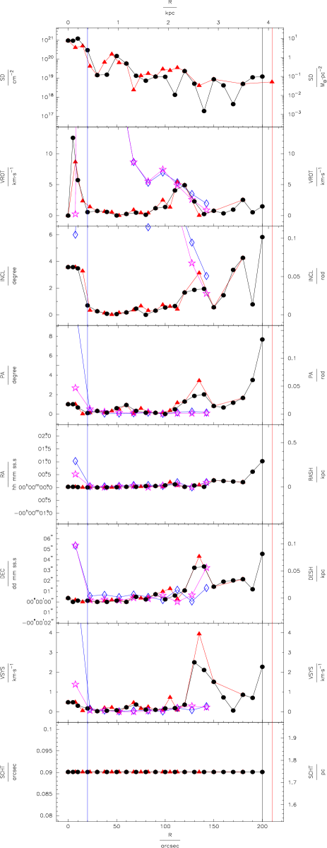
Quantity	Range	method	$N_{{H\textsc{i}}}$	$\frac{N_{{H\textsc{i}}}}{N_{{H\textsc{i}}},exp}$	$v_{\rm rot}$	$i$	$pa$	${\rm RA}$	${\rm DEC}$	$v_{\rm sys}$	$z_{0}$
(1)	(2)	(3)	(4)	(5)	(6)	(7)	(8)	(9)	(10)	(11)	(12)
$\overline{\Delta}$	all	tir	119.82	0.126	1.8	1.2	0.7	0.9	0.7	0.5	0.1
$\sqrt{\overline{\Delta^{2}}}$	all	tir	259.53	0.248	2.8	1.9	1.1	1.5	1.2	1.0	0.1
$\Delta_{\rm max}$	all	tir	965.85	0.966	8.7	4.3	3.4	4.2	4.3	3.9	0.1
$\overline{\Delta}$	70%	tir	17.63	0.037	0.6	0.4	0.3	0.3	0.2	0.2	0.1
$\sqrt{\overline{\Delta^{2}}}$	70%	tir	21.51	0.046	0.8	0.4	0.4	0.4	0.3	0.2	0.1
$\Delta_{\rm max}$	70%	tir	43.33	0.088	1.4	0.8	0.9	0.9	0.7	0.5	0.1
$\overline{\Delta}$	hi	tir	36.71	0.083	1.4	0.8	0.7	1.0	0.8	0.6	0.1
$\sqrt{\overline{\Delta^{2}}}$	hi	tir	56.58	0.129	2.1	1.4	1.1	1.6	1.3	1.1	0.1
$\Delta_{\rm max}$	hi	tir	187.26	0.375	5.4	4.3	3.4	4.2	4.3	3.9	0.1
$\overline{\Delta}$	$8-\sigma$	tir	14.20	0.192	2.7	2.0	1.7	2.1	1.9	1.4	0.1
$\sqrt{\overline{\Delta^{2}}}$	$8-\sigma$	tir	18.60	0.223	3.5	2.5	1.9	2.5	2.3	1.9	0.1
$\Delta_{\rm max}$	$8-\sigma$	tir	36.53	0.375	5.4	4.3	3.4	4.2	4.3	3.9	0.1
$\overline{\Delta}$	excs	tir	6.45
$\sqrt{\overline{\Delta^{2}}}$	excs	tir	6.45
$\Delta_{\rm max}$	excs	tir	6.45
$\overline{\Delta}$	all	pk			34.0	12.8	0.4	1.7	1.1	0.2
$\sqrt{\overline{\Delta^{2}}}$	all	pk			81.3	16.6	0.9	2.7	2.0	0.5
$\Delta_{\rm max}$	all	pk			253.2	39.9	2.7	7.7	5.4	1.4
$\overline{\Delta}$	70%	pk			4.3	7.2	0.1	0.6	0.3	0.1
$\sqrt{\overline{\Delta^{2}}}$	70%	pk			5.2	8.0	0.1	0.7	0.3	0.1
$\Delta_{\rm max}$	70%	pk			8.6	12.9	0.2	1.2	0.6	0.2
$\overline{\Delta}$	hi	pk			37.8	12.7	0.2	1.0	0.6	0.1
$\sqrt{\overline{\Delta^{2}}}$	hi	pk			85.6	16.9	0.2	1.3	1.1	0.1
$\Delta_{\rm max}$	hi	pk			253.2	39.9	0.5	2.9	3.2	0.3
$\overline{\Delta}$	all	m1			21.3	11.7	1.2	2.8	1.1	0.8
$\sqrt{\overline{\Delta^{2}}}$	all	m1			34.9	14.6	3.5	5.1	1.8	2.2
$\Delta_{\rm max}$	all	m1			97.9	33.0	11.0	15.4	5.3	6.9
$\overline{\Delta}$	70%	m1			7.6	6.7	0.1	0.9	0.4	0.1
$\sqrt{\overline{\Delta^{2}}}$	70%	m1			9.7	6.9	0.1	1.0	0.5	0.1
$\Delta_{\rm max}$	70%	m1			21.4	9.2	0.2	1.5	0.7	0.2
$\overline{\Delta}$	hi	m1			20.5	12.3	0.1	1.4	0.6	0.1
$\sqrt{\overline{\Delta^{2}}}$	hi	m1			35.5	15.3	0.2	1.7	0.7	0.1
$\Delta_{\rm max}$	hi	m1			97.9	33.0	0.3	3.2	1.3	0.3

Figure 14: Test 5: asymmetric warp with central shift and shift in sytemic velocity. The scale height is constant with radius, the data cube contains no noise. constant scale height. The results get unreliable at low inclination ($i<25\hbox{${}^{\circ}$}$). ROTCUR: first guess deviates by $10\,{\rm km}\,{\rm s}^{-1}$ in rotation velocity, by $10\hbox{${}^{\circ}$}$ in inclination and position angle, by $10\,{\rm km}\,{\rm s}^{-1}$ in systemic velocity, and by $10\arcsec$ in both central coordinates from the optimal guess. All parameters except expansion velocity were left variable. For symbol- and colour coding see the introduction to this section.

Table 6: Test 5: asymmetric warp with central shift and shift in sytemic velocity. The scale height is constant with radius, the data cube contains no noise. The scale height is constant. Deviation in global dispersion: 0.06 ${\rm km}\,{\rm s}^{-1}$. The results get unreliable at low inclination ($i<25\hbox{${}^{\circ}$}$). ROTCUR: first guess deviates by $10\,{\rm km}\,{\rm s}^{-1}$ in rotation velocity, by $10\hbox{${}^{\circ}$}$ in inclination and position angle, by $10\,{\rm km}\,{\rm s}^{-1}$ in systemic velocity, and by $10\arcsec$ in both central coordinates from the optimal guess. All parameters except expansion velocity were left variable.

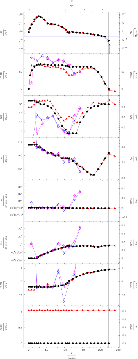
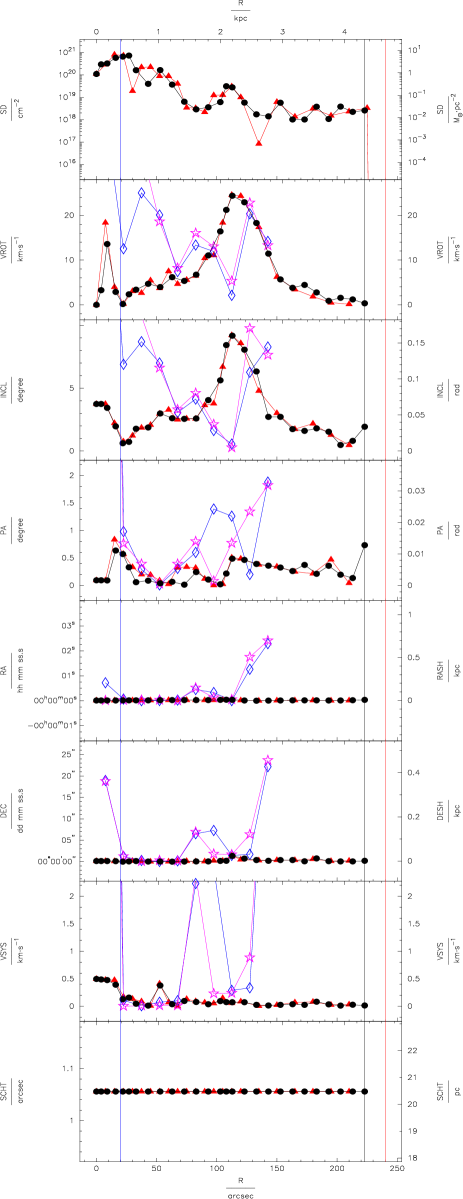
Quantity	Range	method	$N_{{H\textsc{i}}}$	$\frac{N_{{H\textsc{i}}}}{N_{{H\textsc{i}}},exp}$	$v_{\rm rot}$	$i$	$pa$	${\rm RA}$	${\rm DEC}$	$v_{\rm sys}$	$z_{0}$
(1)	(2)	(3)	(4)	(5)	(6)	(7)	(8)	(9)	(10)	(11)	(12)
$\overline{\Delta}$	all	tir	108.87	0.138	7.8	3.3	0.3	0.3	0.2	0.1	1.1
$\sqrt{\overline{\Delta^{2}}}$	all	tir	237.61	0.270	10.8	3.9	0.3	0.3	0.4	0.2	1.1
$\Delta_{\rm max}$	all	tir	808.64	1.103	24.6	9.2	0.8	0.6	1.4	0.5	1.1
$\overline{\Delta}$	70%	tir	8.97	0.042	3.5	2.1	0.2	0.2	0.1	0.1	1.1
$\sqrt{\overline{\Delta^{2}}}$	70%	tir	14.27	0.052	4.2	2.3	0.2	0.2	0.1	0.1	1.1
$\Delta_{\rm max}$	70%	tir	40.55	0.087	7.5	3.6	0.3	0.3	0.2	0.1	1.1
$\overline{\Delta}$	hi	tir	75.50	0.066	7.9	3.3	0.3	0.3	0.3	0.1	1.1
$\sqrt{\overline{\Delta^{2}}}$	hi	tir	181.88	0.094	10.8	4.0	0.3	0.3	0.4	0.1	1.1
$\Delta_{\rm max}$	hi	tir	736.63	0.305	24.6	9.2	0.6	0.6	1.4	0.4	1.1
$\overline{\Delta}$	$8-\sigma$	tir	5.86	0.084	9.8	3.9	0.3	0.2	0.5	0.0	1.1
$\sqrt{\overline{\Delta^{2}}}$	$8-\sigma$	tir	10.51	0.123	13.9	5.0	0.4	0.3	0.6	0.1	1.1
$\Delta_{\rm max}$	$8-\sigma$	tir	30.54	0.305	24.6	9.2	0.5	0.6	1.4	0.1	1.1
$\overline{\Delta}$	$2-\sigma$	tir	1.90	0.074	0.1	0.5	0.0	0.2	0.2	0.0	1.1
$\sqrt{\overline{\Delta^{2}}}$	$2-\sigma$	tir	2.36	0.074	0.1	0.5	0.0	0.2	0.2	0.0	1.1
$\Delta_{\rm max}$	$2-\sigma$	tir	3.35	0.074	0.1	0.5	0.0	0.2	0.2	0.0	1.1
$\overline{\Delta}$	excs	tir	1.67
$\sqrt{\overline{\Delta^{2}}}$	excs	tir	2.37
$\Delta_{\rm max}$	excs	tir	3.35
$\overline{\Delta}$	all	pk			23.8	8.5	2.3	7.4	6.1	2.7
$\sqrt{\overline{\Delta^{2}}}$	all	pk			30.3	10.8	5.2	14.3	10.0	5.7
$\Delta_{\rm max}$	all	pk			33.6	22.9	16.2	36.1	23.7	16.7
$\overline{\Delta}$	70%	pk			13.9	4.9	0.5	0.5	1.7	0.2
$\sqrt{\overline{\Delta^{2}}}$	70%	pk			14.9	5.8	0.6	0.8	2.6	0.4
$\Delta_{\rm max}$	70%	pk			22.8	9.8	0.8	1.9	6.4	0.9
$\overline{\Delta}$	hi	pk			22.7	6.9	0.7	8.2	4.7	1.1
$\sqrt{\overline{\Delta^{2}}}$	hi	pk			29.9	8.4	0.9	15.1	8.5	2.2
$\Delta_{\rm max}$	hi	pk			72.7	17.1	1.8	36.1	23.7	6.1
$\overline{\Delta}$	all	m1			16.9	7.3	3.7	7.7	6.0	3.6
$\sqrt{\overline{\Delta^{2}}}$	all	m1			20.0	9.9	9.6	13.1	9.8	7.9
$\Delta_{\rm max}$	all	m1			42.6	26.0	30.1	34.3	22.2	24.0
$\overline{\Delta}$	70%	m1			11.7	4.2	0.5	1.9	1.6	0.5
$\sqrt{\overline{\Delta^{2}}}$	70%	m1			12.8	4.9	0.7	3.2	2.7	0.9
$\Delta_{\rm max}$	70%	m1			20.1	7.0	1.3	6.7	6.5	2.2
$\overline{\Delta}$	hi	m1			14.1	5.2	0.8	7.4	4.5	1.3
$\sqrt{\overline{\Delta^{2}}}$	hi	m1			15.6	5.9	1.0	13.4	8.1	2.3
$\Delta_{\rm max}$	hi	m1			25.0	8.7	1.9	34.3	22.2	6.0

Figure 15: Test 6: warp with central/sytemic velocity shift and variable scale height without noise added to the data cube. ROTCUR: first guess deviates by $5\,{\rm km}\,{\rm s}^{-1}$ in rotation velocity, by $5\hbox{${}^{\circ}$}$ in inclination and position angle, by $5\,{\rm km}\,{\rm s}^{-1}$ in systemic velocity, and by $5\arcsec$ in both central coordinates from the optimal guess. All parameters except expansion velocity were left variable. For symbol- and colour coding see the introduction to this section.

Table 7: Test 6: warp with central/sytemic velocity shift and variable scale height without noise added to the data cube. Deviation in global dispersion: 0.06 ${\rm km}\,{\rm s}^{-1}$. ROTCUR: first guess deviates by $5\,{\rm km}\,{\rm s}^{-1}$ in rotation velocity, by $5\hbox{${}^{\circ}$}$ in inclination and position angle, by $5\,{\rm km}\,{\rm s}^{-1}$ in systemic velocity, and by $5\arcsec$ in both central coordinates from the optimal guess. All parameters except expansion velocity were left variable.

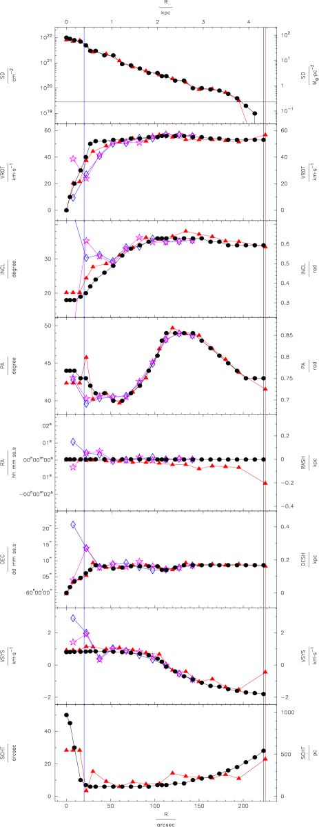
Quantity	Range	method	$N_{{H\textsc{i}}}$	$\frac{N_{{H\textsc{i}}}}{N_{{H\textsc{i}}},exp}$	$v_{\rm rot}$	$i$	$pa$	${\rm RA}$	${\rm DEC}$	$v_{\rm sys}$	$z_{0}$
(1)	(2)	(3)	(4)	(5)	(6)	(7)	(8)	(9)	(10)	(11)	(12)
$\overline{\Delta}$	all	tir	265.41	0.083	2.5	1.7	0.7	3.2	0.4	0.2	5.4
$\sqrt{\overline{\Delta^{2}}}$	all	tir	569.74	0.096	3.2	2.1	1.0	4.0	0.5	0.2	7.9
$\Delta_{\rm max}$	all	tir	1895.32	0.190	7.1	4.7	2.9	8.1	1.4	0.4	21.7
$\overline{\Delta}$	70%	tir	12.61	0.058	1.4	1.1	0.2	1.8	0.2	0.1	2.4
$\sqrt{\overline{\Delta^{2}}}$	70%	tir	15.59	0.066	1.6	1.2	0.3	2.2	0.2	0.1	2.9
$\Delta_{\rm max}$	70%	tir	25.18	0.110	2.7	2.1	0.7	4.4	0.4	0.3	6.2
$\overline{\Delta}$	hi	tir	63.43	0.070	2.2	1.7	0.5	3.8	0.4	0.2	3.3
$\sqrt{\overline{\Delta^{2}}}$	hi	tir	123.19	0.081	2.8	2.1	0.9	4.4	0.6	0.2	4.3
$\Delta_{\rm max}$	hi	tir	329.48	0.142	6.7	4.7	2.9	8.1	1.4	0.4	9.3
$\overline{\Delta}$	$8-\sigma$	tir	4.67	0.081	1.4	1.2	0.2	6.8	0.2	0.2	2.9
$\sqrt{\overline{\Delta^{2}}}$	$8-\sigma$	tir	6.10	0.088	1.4	1.2	0.2	6.8	0.3	0.2	4.0
$\Delta_{\rm max}$	$8-\sigma$	tir	11.50	0.115	2.0	1.5	0.4	8.1	0.4	0.4	7.6
$\overline{\Delta}$	$2-\sigma$	tir	2.03	0.112	1.6	1.0	0.0	7.0	0.4	0.1	7.6
$\sqrt{\overline{\Delta^{2}}}$	$2-\sigma$	tir	2.85	0.112	1.6	1.0	0.0	7.0	0.4	0.1	7.6
$\Delta_{\rm max}$	$2-\sigma$	tir	4.03	0.112	1.6	1.0	0.0	7.0	0.4	0.1	7.6
$\overline{\Delta}$	excs	tir	0.03
$\sqrt{\overline{\Delta^{2}}}$	excs	tir	0.03
$\Delta_{\rm max}$	excs	tir	0.03
$\overline{\Delta}$	all	pk			5.9	3.7	0.6	2.5	1.3	0.3
$\sqrt{\overline{\Delta^{2}}}$	all	pk			9.4	5.9	1.0	3.7	2.5	0.4
$\Delta_{\rm max}$	all	pk			21.6	15.1	2.6	7.0	7.7	1.1
$\overline{\Delta}$	70%	pk			1.5	1.0	0.3	0.8	0.3	0.1
$\sqrt{\overline{\Delta^{2}}}$	70%	pk			1.7	1.2	0.4	1.0	0.5	0.1
$\Delta_{\rm max}$	70%	pk			3.1	2.3	0.6	1.9	0.9	0.2
$\overline{\Delta}$	hi	pk			4.2	3.1	0.6	2.0	1.3	0.2
$\sqrt{\overline{\Delta^{2}}}$	hi	pk			6.8	5.5	1.0	3.1	2.7	0.4
$\Delta_{\rm max}$	hi	pk			17.1	15.1	2.6	6.9	7.7	1.1
$\overline{\Delta}$	all	m1			4.3	4.8	0.7	3.0	3.1	0.4
$\sqrt{\overline{\Delta^{2}}}$	all	m1			6.3	8.9	1.2	5.4	6.3	0.8
$\Delta_{\rm max}$	all	m1			14.0	25.2	3.3	15.4	18.2	2.1
$\overline{\Delta}$	70%	m1			1.4	0.9	0.3	0.8	0.5	0.1
$\sqrt{\overline{\Delta^{2}}}$	70%	m1			1.7	1.0	0.4	1.0	0.7	0.1
$\Delta_{\rm max}$	70%	m1			3.0	1.6	0.7	2.0	1.3	0.2
$\overline{\Delta}$	hi	m1			3.9	2.5	0.7	1.7	1.4	0.2
$\sqrt{\overline{\Delta^{2}}}$	hi	m1			6.2	4.1	1.2	2.5	2.7	0.4
$\Delta_{\rm max}$	hi	m1			14.0	10.1	3.3	5.4	7.7	1.2

Figure 16: Test 7: asymmetric warp with central/sytemic velocity shift and variable scale height, noise added to the data cube. ROTCUR: optimal first guesses. All parameters except expansion velocity were left variable. For symbol- and colour coding see the introduction to this section.

Table 8: Test 7: asymmetric warp with central/sytemic velocity shift and variable scale height, noise added to the data cube. Deviation in global dispersion: below 0.01 ${\rm km}\,{\rm s}^{-1}$. ROTCUR: optimal first guesses. All parameters except expansion velocity were left variable.

Quantity	Range	method	$N_{{H\textsc{i}}}$	$\frac{N_{{H\textsc{i}}}}{N_{{H\textsc{i}}},exp}$	$v_{\rm rot}$	$i$	$pa$	${\rm RA}$	${\rm DEC}$	$v_{\rm sys}$	$z_{0}$
(1)	(2)	(3)	(4)	(5)	(6)	(7)	(8)	(9)	(10)	(11)	(12)
$\overline{\Delta}$	all	tir	30.11	0.156	3.6	1.5	2.2	0.5	0.4	0.2	2.6
$\sqrt{\overline{\Delta^{2}}}$	all	tir	48.80	0.315	4.7	1.8	3.1	1.1	0.6	0.3	3.9
$\Delta_{\rm max}$	all	tir	156.23	0.980	13.9	3.9	8.2	3.8	1.8	0.8	10.2
$\overline{\Delta}$	70%	tir	8.62	0.039	2.1	0.9	1.1	0.1	0.2	0.1	1.0
$\sqrt{\overline{\Delta^{2}}}$	70%	tir	11.87	0.048	2.4	1.0	1.3	0.2	0.2	0.1	1.3
$\Delta_{\rm max}$	70%	tir	32.38	0.082	3.6	1.4	2.3	0.3	0.4	0.2	2.6
$\overline{\Delta}$	hi	tir	28.24	0.060	3.1	1.4	1.4	0.4	0.3	0.2	2.6
$\sqrt{\overline{\Delta^{2}}}$	hi	tir	47.10	0.084	3.6	1.7	1.7	0.8	0.6	0.2	3.7
$\Delta_{\rm max}$	hi	tir	156.23	0.249	7.7	3.9	3.9	2.6	1.8	0.8	10.2
$\overline{\Delta}$	$8-\sigma$	tir	8.89	0.150	5.6	2.9	1.6	1.5	1.0	0.4	6.7
$\sqrt{\overline{\Delta^{2}}}$	$8-\sigma$	tir	14.00	0.166	5.7	3.1	1.8	2.1	1.2	0.5	7.2
$\Delta_{\rm max}$	$8-\sigma$	tir	32.38	0.249	7.7	3.9	2.7	3.8	1.8	0.8	10.2
$\overline{\Delta}$	$2-\sigma$	tir	0.95	0.210	5.4	3.5	2.7	3.8	1.7	0.7	8.5
$\sqrt{\overline{\Delta^{2}}}$	$2-\sigma$	tir	1.34	0.210	5.4	3.5	2.7	3.8	1.7	0.7	8.5
$\Delta_{\rm max}$	$2-\sigma$	tir	1.89	0.210	5.4	3.5	2.7	3.8	1.7	0.7	8.5
$\overline{\Delta}$	$0.5-\sigma$	tir	0.95	0.210	5.4	3.5	2.7	3.8	1.7	0.7	8.5
$\sqrt{\overline{\Delta^{2}}}$	$0.5-\sigma$	tir	1.34	0.210	5.4	3.5	2.7	3.8	1.7	0.7	8.5
$\Delta_{\rm max}$	$0.5-\sigma$	tir	1.89	0.210	5.4	3.5	2.7	3.8	1.7	0.7	8.5
$\overline{\Delta}$	excs	tir	0.00
$\sqrt{\overline{\Delta^{2}}}$	excs	tir	0.00
$\Delta_{\rm max}$	excs	tir	0.00
$\overline{\Delta}$	all	pk			28.6	4.6	2.1	3.0	1.3	0.2
$\sqrt{\overline{\Delta^{2}}}$	all	pk			59.5	7.3	3.2	4.3	1.6	0.5
$\Delta_{\rm max}$	all	pk			178.2	17.3	8.7	7.8	2.6	1.4
$\overline{\Delta}$	70%	pk			3.4	1.2	1.1	1.3	0.7	0.1
$\sqrt{\overline{\Delta^{2}}}$	70%	pk			4.9	1.8	1.2	1.9	0.9	0.1
$\Delta_{\rm max}$	70%	pk			9.4	3.4	1.8	4.4	1.6	0.2
$\overline{\Delta}$	hi	pk			11.9	3.2	1.4	3.2	1.3	0.1
$\sqrt{\overline{\Delta^{2}}}$	hi	pk			20.2	5.1	1.6	4.5	1.6	0.1
$\Delta_{\rm max}$	hi	pk			44.1	10.2	2.8	7.8	2.6	0.3
$\overline{\Delta}$	all	m1			15.3	3.2	2.1	3.0	1.4	0.3
$\sqrt{\overline{\Delta^{2}}}$	all	m1			30.7	5.6	2.5	4.4	1.6	0.5
$\Delta_{\rm max}$	all	m1			92.5	15.7	4.8	8.1	2.6	1.6
$\overline{\Delta}$	70%	m1			3.6	0.9	1.5	1.2	1.0	0.1
$\sqrt{\overline{\Delta^{2}}}$	70%	m1			4.2	1.1	1.7	2.2	1.1	0.1
$\Delta_{\rm max}$	70%	m1			7.0	1.7	2.9	5.5	1.6	0.2
$\overline{\Delta}$	hi	m1			15.9	3.4	1.8	3.2	1.5	0.1
$\sqrt{\overline{\Delta^{2}}}$	hi	m1			32.1	5.9	2.1	4.6	1.7	0.2
$\Delta_{\rm max}$	hi	m1			92.5	15.7	3.2	8.1	2.6	0.3

Figure 17: Test 8: flat disk with constant scale height, centre, and systemic velocity. Noise was added to the data cube. ROTCUR: input model with optimal guesses. Only the rotation velocity and the orientation parameters were fitted. For symbol- and colour coding see the introduction to this section.

Table 9: Test 8: flat disk with constant scale height, centre, and systemic velocity. Noise was added to the data cube. Deviation in global dispersion: 0.12 ${\rm km}\,{\rm s}^{-1}$. ROTCUR: input model with optimal guesses. Only the rotation velocity and the orientation parameters were fitted.

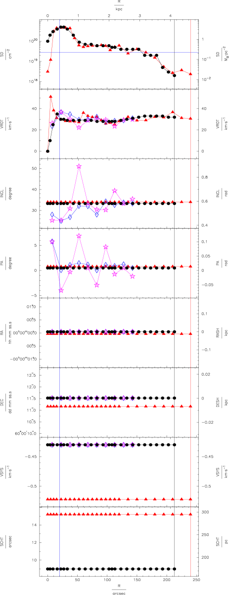
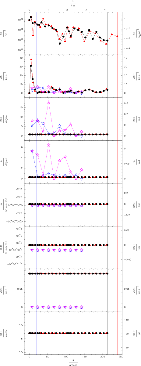
Quantity	Range	method	$N_{{H\textsc{i}}}$	$\frac{N_{{H\textsc{i}}}}{N_{{H\textsc{i}}},exp}$	$v_{\rm rot}$	$i$	$pa$	${\rm RA}$	${\rm DEC}$	$v_{\rm sys}$	$z_{0}$
(1)	(2)	(3)	(4)	(5)	(6)	(7)	(8)	(9)	(10)	(11)	(12)
$\overline{\Delta}$	all	tir	28.90	0.253	4.1	0.7	0.3	1.2	0.4	0.1	6.2
$\sqrt{\overline{\Delta^{2}}}$	all	tir	55.43	0.358	8.6	0.7	0.3	1.2	0.4	0.1	6.2
$\Delta_{\rm max}$	all	tir	207.90	0.969	38.2	0.7	0.3	1.2	0.4	0.1	6.2
$\overline{\Delta}$	70%	tir	6.87	0.116	1.4	0.7	0.3	1.2	0.4	0.1	6.2
$\sqrt{\overline{\Delta^{2}}}$	70%	tir	9.57	0.147	1.6	0.7	0.3	1.2	0.4	0.1	6.2
$\Delta_{\rm max}$	70%	tir	19.57	0.313	2.8	0.7	0.3	1.2	0.4	0.1	6.2
$\overline{\Delta}$	hi	tir	22.29	0.187	2.3	0.7	0.3	1.2	0.4	0.1	6.2
$\sqrt{\overline{\Delta^{2}}}$	hi	tir	37.63	0.242	2.9	0.7	0.3	1.2	0.4	0.1	6.2
$\Delta_{\rm max}$	hi	tir	130.94	0.426	7.1	0.7	0.3	1.2	0.4	0.1	6.2
$\overline{\Delta}$	$8-\sigma$	tir	8.82	0.203	2.7	0.7	0.3	1.2	0.4	0.1	6.2
$\sqrt{\overline{\Delta^{2}}}$	$8-\sigma$	tir	12.77	0.249	3.2	0.7	0.3	1.2	0.4	0.1	6.2
$\Delta_{\rm max}$	$8-\sigma$	tir	32.78	0.426	7.1	0.7	0.3	1.2	0.4	0.1	6.2
$\overline{\Delta}$	$2-\sigma$	tir	3.31	0.248	2.6	0.7	0.3	1.2	0.4	0.1	6.2
$\sqrt{\overline{\Delta^{2}}}$	$2-\sigma$	tir	4.17	0.263	3.1	0.7	0.3	1.2	0.4	0.1	6.2
$\Delta_{\rm max}$	$2-\sigma$	tir	7.99	0.400	4.8	0.7	0.3	1.2	0.4	0.1	6.2
$\overline{\Delta}$	$0.5-\sigma$	tir	1.83	0.183	2.9	0.7	0.3	1.2	0.4	0.1	6.2
$\sqrt{\overline{\Delta^{2}}}$	$0.5-\sigma$	tir	2.25	0.183	3.4	0.7	0.3	1.2	0.4	0.1	6.2
$\Delta_{\rm max}$	$0.5-\sigma$	tir	3.71	0.186	4.8	0.7	0.3	1.2	0.4	0.1	6.2
$\overline{\Delta}$	excs	tir	3.03
$\sqrt{\overline{\Delta^{2}}}$	excs	tir	3.11
$\Delta_{\rm max}$	excs	tir	3.71
$\overline{\Delta}$	all	pk			3.0	5.0	2.7	0.0	0.0	0.0
$\sqrt{\overline{\Delta^{2}}}$	all	pk			3.9	7.1	3.5	0.0	0.0	0.0
$\Delta_{\rm max}$	all	pk			6.8	17.7	6.4	0.0	0.0	0.0
$\overline{\Delta}$	70%	pk			1.5	2.4	1.6	0.0	0.0	0.0
$\sqrt{\overline{\Delta^{2}}}$	70%	pk			2.0	3.0	2.2	0.0	0.0	0.0
$\Delta_{\rm max}$	70%	pk			4.6	6.1	4.2	0.0	0.0	0.0
$\overline{\Delta}$	hi	pk			2.6	4.7	2.5	0.0	0.0	0.0
$\sqrt{\overline{\Delta^{2}}}$	hi	pk			3.7	7.0	3.3	0.0	0.0	0.0
$\Delta_{\rm max}$	hi	pk			6.8	17.7	6.4	0.0	0.0	0.0
$\overline{\Delta}$	all	m1			2.3	3.0	1.0	0.0	0.0	0.0
$\sqrt{\overline{\Delta^{2}}}$	all	m1			3.3	4.1	1.8	0.0	0.0	0.0
$\Delta_{\rm max}$	all	m1			6.7	8.3	5.3	0.0	0.0	0.0
$\overline{\Delta}$	70%	m1			0.9	1.4	0.5	0.0	0.0	0.0
$\sqrt{\overline{\Delta^{2}}}$	70%	m1			1.3	2.2	0.5	0.0	0.0	0.0
$\Delta_{\rm max}$	70%	m1			3.1	5.3	0.7	0.0	0.0	0.0
$\overline{\Delta}$	hi	m1			2.2	2.7	0.5	0.0	0.0	0.0
$\sqrt{\overline{\Delta^{2}}}$	hi	m1			3.3	4.0	0.6	0.0	0.0	0.0
$\Delta_{\rm max}$	hi	m1			6.7	8.3	1.0	0.0	0.0	0.0

Figure 18: Test 9: slight symmetric warp without central/sytemic velocity shift and variable scale height, noise added. ROTCUR: input model with optimal guesses. Only the rotation velocity and the orientation parameters were fitted. For symbol- and colour coding see the introduction to this section.

Table 10: Test 9: slight symmetric warp without central/sytemic velocity shift and variable scale height, noise added. Deviation in global dispersion: 0.09 ${\rm km}\,{\rm s}^{-1}$. ROTCUR: input model with optimal guesses. Only the rotation velocity and the orientation parameters were fitted.

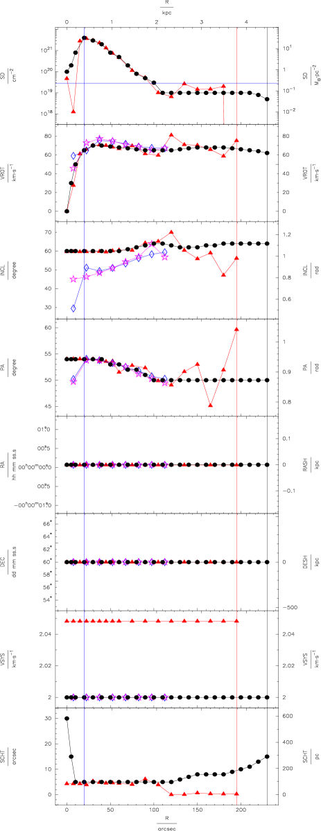
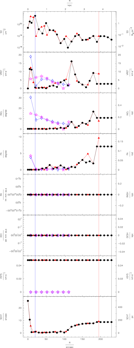
Quantity	Range	method	$N_{{H\textsc{i}}}$	$\frac{N_{{H\textsc{i}}}}{N_{{H\textsc{i}}},exp}$	$v_{\rm rot}$	$i$	$pa$	${\rm RA}$	${\rm DEC}$	$v_{\rm sys}$	$z_{0}$
(1)	(2)	(3)	(4)	(5)	(6)	(7)	(8)	(9)	(10)	(11)	(12)
$\overline{\Delta}$	all	tir	72.06	0.423	4.2	2.8	1.5	0.1	0.0	0.0	4.5
$\sqrt{\overline{\Delta^{2}}}$	all	tir	157.30	0.625	6.1	5.0	2.8	0.1	0.0	0.0	7.5
$\Delta_{\rm max}$	all	tir	498.73	1.674	16.2	16.8	9.7	0.1	0.0	0.0	25.7
$\overline{\Delta}$	70%	tir	12.01	0.157	1.5	0.6	0.4	0.1	0.0	0.0	1.5
$\sqrt{\overline{\Delta^{2}}}$	70%	tir	14.93	0.232	2.0	0.7	0.6	0.1	0.0	0.0	2.3
$\Delta_{\rm max}$	70%	tir	33.38	0.491	3.7	1.3	1.4	0.1	0.0	0.0	5.7
$\overline{\Delta}$	hi	tir	32.72	0.052	1.3	0.6	0.6	0.1	0.0	0.0	0.6
$\sqrt{\overline{\Delta^{2}}}$	hi	tir	40.64	0.075	1.8	0.7	0.8	0.1	0.0	0.0	0.7
$\Delta_{\rm max}$	hi	tir	75.55	0.183	3.7	1.3	1.5	0.1	0.0	0.0	1.1
$\overline{\Delta}$	$8-\sigma$	tir	9.78	0.637	6.2	5.2	2.7	0.1	0.0	0.0	5.2
$\sqrt{\overline{\Delta^{2}}}$	$8-\sigma$	tir	12.02	0.797	7.5	7.1	3.9	0.1	0.0	0.0	6.0
$\Delta_{\rm max}$	$8-\sigma$	tir	25.56	1.674	16.2	16.8	9.7	0.1	0.0	0.0	9.2
$\overline{\Delta}$	$2-\sigma$	tir	8.56	0.786	6.9	6.4	3.2	0.1	0.0	0.0	6.3
$\sqrt{\overline{\Delta^{2}}}$	$2-\sigma$	tir	9.57	0.901	8.3	8.0	4.4	0.1	0.0	0.0	6.8
$\Delta_{\rm max}$	$2-\sigma$	tir	16.74	1.674	16.2	16.8	9.7	0.1	0.0	0.0	9.2
$\overline{\Delta}$	excs	tir	8.25
$\sqrt{\overline{\Delta^{2}}}$	excs	tir	8.50
$\Delta_{\rm max}$	excs	tir	10.00
$\overline{\Delta}$	all	pk			4.3	8.5	0.8	0.0	0.0	0.0
$\sqrt{\overline{\Delta^{2}}}$	all	pk			4.9	9.7	1.6	0.0	0.0	0.0
$\Delta_{\rm max}$	all	pk			2.2	15.0	4.3	0.0	0.0	0.0
$\overline{\Delta}$	70%	pk			2.9	5.6	0.2	0.0	0.0	0.0
$\sqrt{\overline{\Delta^{2}}}$	70%	pk			3.5	6.3	0.2	0.0	0.0	0.0
$\Delta_{\rm max}$	70%	pk			5.7	9.1	0.3	0.0	0.0	0.0
$\overline{\Delta}$	hi	pk			4.5	7.7	0.2	0.0	0.0	0.0
$\sqrt{\overline{\Delta^{2}}}$	hi	pk			5.1	8.9	0.3	0.0	0.0	0.0
$\Delta_{\rm max}$	hi	pk			7.3	13.7	0.6	0.0	0.0	0.0
$\overline{\Delta}$	all	m1			5.5	10.3	0.7	0.0	0.0	0.0
$\sqrt{\overline{\Delta^{2}}}$	all	m1			7.6	13.0	1.4	0.0	0.0	0.0
$\Delta_{\rm max}$	all	m1			19.0	30.6	3.8	0.0	0.0	0.0
$\overline{\Delta}$	70%	m1			2.8	6.4	0.2	0.0	0.0	0.0
$\sqrt{\overline{\Delta^{2}}}$	70%	m1			3.0	6.6	0.2	0.0	0.0	0.0
$\Delta_{\rm max}$	70%	m1			4.6	8.9	0.3	0.0	0.0	0.0
$\overline{\Delta}$	hi	m1			3.8	7.9	0.2	0.0	0.0	0.0
$\sqrt{\overline{\Delta^{2}}}$	hi	m1			4.1	8.1	0.3	0.0	0.0	0.0
$\Delta_{\rm max}$	hi	m1			5.7	10.6	0.5	0.0	0.0	0.0

Figure 19: Test 10: slight warp without central/sytemic velocity shift and variable scale height, noise added to the data cube. ROTCUR: input model with optimal guesses. Only rotation velocity, position angle, and inclination were fitted. For symbol- and colour coding see the introduction to this section.

Table 11: Test 10: slight warp without central/sytemic velocity shift and variable scale height, noise added to the data cube. Deviation in global dispersion: 0.12 ${\rm km}\,{\rm s}^{-1}$. ROTCUR: input model with optimal guesses. Only rotation velocity, position angle, and inclination were fitted.

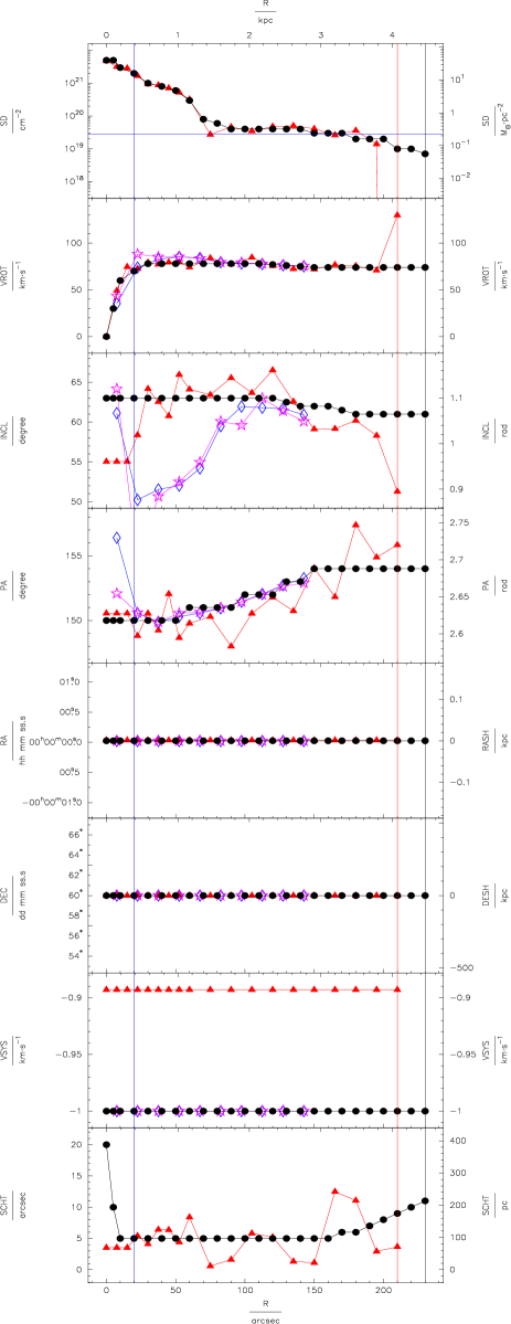
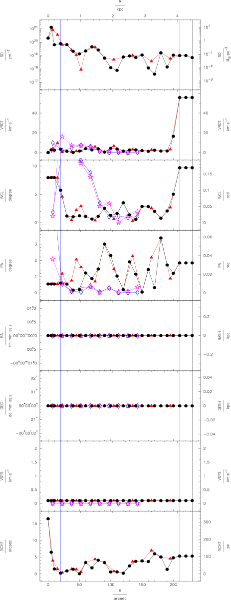
Quantity	Range	method	$N_{{H\textsc{i}}}$	$\frac{N_{{H\textsc{i}}}}{N_{{H\textsc{i}}},exp}$	$v_{\rm rot}$	$i$	$pa$	${\rm RA}$	${\rm DEC}$	$v_{\rm sys}$	$z_{0}$
(1)	(2)	(3)	(4)	(5)	(6)	(7)	(8)	(9)	(10)	(11)	(12)
$\overline{\Delta}$	all	tir	89.66	0.240	5.6	3.3	1.3	0.2	0.0	0.1	3.6
$\sqrt{\overline{\Delta^{2}}}$	all	tir	215.03	0.362	13.3	4.4	1.6	0.2	0.0	0.1	5.1
$\Delta_{\rm max}$	all	tir	834.24	1.000	55.8	9.7	3.4	0.2	0.0	0.1	16.5
$\overline{\Delta}$	70%	tir	10.46	0.094	1.5	1.6	0.8	0.2	0.0	0.1	2.0
$\sqrt{\overline{\Delta^{2}}}$	70%	tir	12.46	0.116	1.8	1.9	0.9	0.2	0.0	0.1	2.4
$\Delta_{\rm max}$	70%	tir	25.22	0.209	3.2	2.9	1.6	0.2	0.0	0.1	4.0
$\overline{\Delta}$	hi	tir	21.19	0.159	2.5	2.0	1.3	0.2	0.0	0.1	2.4
$\sqrt{\overline{\Delta^{2}}}$	hi	tir	30.10	0.229	3.1	2.4	1.6	0.2	0.0	0.1	3.1
$\Delta_{\rm max}$	hi	tir	65.39	0.610	6.7	4.6	3.0	0.2	0.0	0.1	7.0
$\overline{\Delta}$	$8-\sigma$	tir	11.92	0.395	8.3	2.6	1.6	0.2	0.0	0.1	3.8
$\sqrt{\overline{\Delta^{2}}}$	$8-\sigma$	tir	16.09	0.491	18.0	3.7	1.9	0.2	0.0	0.1	4.3
$\Delta_{\rm max}$	$8-\sigma$	tir	42.69	1.000	55.8	9.7	3.4	0.2	0.0	0.1	7.0
$\overline{\Delta}$	$2-\sigma$	tir	9.38	0.520	13.0	3.7	1.7	0.2	0.0	0.1	5.2
$\sqrt{\overline{\Delta^{2}}}$	$2-\sigma$	tir	10.33	0.616	25.0	4.8	2.0	0.2	0.0	0.1	5.3
$\Delta_{\rm max}$	$2-\sigma$	tir	16.21	1.000	55.8	9.7	3.4	0.2	0.0	0.1	7.0
$\overline{\Delta}$	excs	tir	8.50
$\sqrt{\overline{\Delta^{2}}}$	excs	tir	8.63
$\Delta_{\rm max}$	excs	tir	10.00
$\overline{\Delta}$	all	pk			4.1	6.2	0.4	0.0	0.0	0.0
$\sqrt{\overline{\Delta^{2}}}$	all	pk			6.3	8.9	0.7	0.0	0.0	0.0
$\Delta_{\rm max}$	all	pk			16.0	20.7	2.1	0.0	0.0	0.0
$\overline{\Delta}$	70%	pk			1.5	2.7	0.2	0.0	0.0	0.0
$\sqrt{\overline{\Delta^{2}}}$	70%	pk			2.3	3.6	0.2	0.0	0.0	0.0
$\Delta_{\rm max}$	70%	pk			5.5	8.0	0.3	0.0	0.0	0.0
$\overline{\Delta}$	hi	pk			4.4	6.8	0.2	0.0	0.0	0.0
$\sqrt{\overline{\Delta^{2}}}$	hi	pk			6.6	9.3	0.3	0.0	0.0	0.0
$\Delta_{\rm max}$	hi	pk			16.0	20.7	0.6	0.0	0.0	0.0
$\overline{\Delta}$	all	m1			3.2	5.4	0.8	0.0	0.0	0.0
$\sqrt{\overline{\Delta^{2}}}$	all	m1			4.6	7.2	2.0	0.0	0.0	0.0
$\Delta_{\rm max}$	all	m1			6.1	12.8	6.4	0.0	0.0	0.0
$\overline{\Delta}$	70%	m1			1.2	2.6	0.1	0.0	0.0	0.0
$\sqrt{\overline{\Delta^{2}}}$	70%	m1			2.0	3.7	0.1	0.0	0.0	0.0
$\Delta_{\rm max}$	70%	m1			4.6	8.8	0.3	0.0	0.0	0.0
$\overline{\Delta}$	hi	m1			2.4	5.8	0.2	0.0	0.0	0.0
$\sqrt{\overline{\Delta^{2}}}$	hi	m1			3.6	7.5	0.3	0.0	0.0	0.0
$\Delta_{\rm max}$	hi	m1			7.3	12.8	0.5	0.0	0.0	0.0

Figure 20: Test 11: symmetric warp without central/sytemic velocity shift, constant scale height. The data cube contains no noise. ROTCUR: input model with optimal guesses. Only the rotation velocity and the orientation parameters were fitted. For symbol- and colour coding see the introduction to this section.

Table 12: Test 11: symmetric warp without central/sytemic velocity shift, constant scale height. The data cube contains no noise. Deviation in global dispersion: 0.01 ${\rm km}\,{\rm s}^{-1}$. ROTCUR: input model with optimal guesses. Only the rotation velocity and the orientation parameters were fitted.

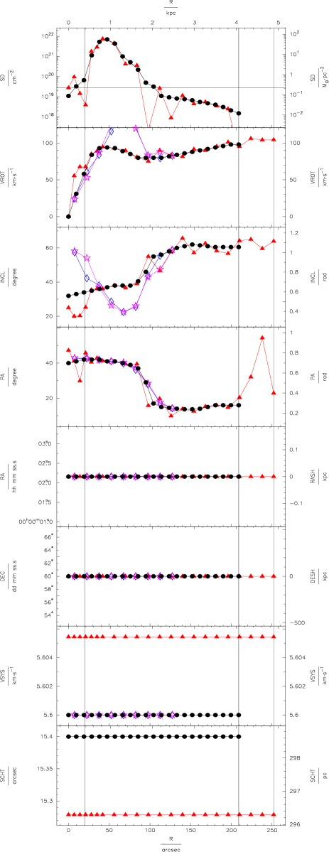
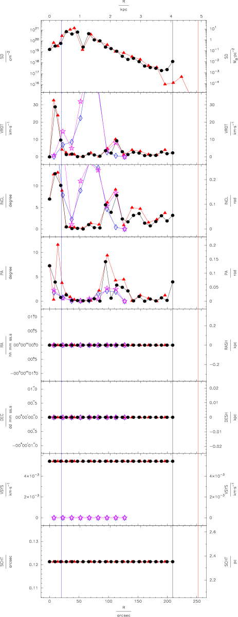
Quantity	Range	method	$N_{{H\textsc{i}}}$	$\frac{N_{{H\textsc{i}}}}{N_{{H\textsc{i}}},exp}$	$v_{\rm rot}$	$i$	$pa$	${\rm RA}$	${\rm DEC}$	$v_{\rm sys}$	$z_{0}$
(1)	(2)	(3)	(4)	(5)	(6)	(7)	(8)	(9)	(10)	(11)	(12)
$\overline{\Delta}$	all	tir	193.54	0.629	5.5	4.4	2.7	0.0	0.0	0.0	0.1
$\sqrt{\overline{\Delta^{2}}}$	all	tir	434.19	0.874	10.1	6.0	4.3	0.0	0.0	0.0	0.1
$\Delta_{\rm max}$	all	tir	1489.84	2.540	32.6	13.1	11.6	0.0	0.0	0.0	0.1
$\overline{\Delta}$	70%	tir	9.06	0.307	1.6	1.8	0.7	0.0	0.0	0.0	0.1
$\sqrt{\overline{\Delta^{2}}}$	70%	tir	15.98	0.378	2.0	2.5	1.0	0.0	0.0	0.0	0.1
$\Delta_{\rm max}$	70%	tir	44.10	0.685	4.0	5.0	2.2	0.0	0.0	0.0	0.1
$\overline{\Delta}$	hi	tir	514.06	0.497	2.1	2.4	2.3	0.0	0.0	0.0	0.1
$\sqrt{\overline{\Delta^{2}}}$	hi	tir	719.46	0.598	2.6	3.9	3.7	0.0	0.0	0.0	0.1
$\Delta_{\rm max}$	hi	tir	1489.84	0.995	4.8	8.9	9.4	0.0	0.0	0.0	0.1
$\overline{\Delta}$	$8-\sigma$	tir	5.79	0.448	3.8	4.2	2.7	0.0	0.0	0.0	0.1
$\sqrt{\overline{\Delta^{2}}}$	$8-\sigma$	tir	13.35	0.572	4.7	4.9	4.0	0.0	0.0	0.0	0.1
$\Delta_{\rm max}$	$8-\sigma$	tir	44.10	0.995	10.2	9.2	9.4	0.0	0.0	0.0	0.1
$\overline{\Delta}$	$2-\sigma$	tir	2.31	0.370	3.6	3.9	1.7	0.0	0.0	0.0	0.1
$\sqrt{\overline{\Delta^{2}}}$	$2-\sigma$	tir	4.22	0.482	4.6	4.7	2.4	0.0	0.0	0.0	0.1
$\Delta_{\rm max}$	$2-\sigma$	tir	10.57	0.902	10.2	9.2	4.5	0.0	0.0	0.0	0.1
$\overline{\Delta}$	$0.5-\sigma$	tir	1.48	0.317	2.5	3.0	1.3	0.0	0.0	0.0	0.1
$\sqrt{\overline{\Delta^{2}}}$	$0.5-\sigma$	tir	2.90	0.439	2.8	3.4	2.0	0.0	0.0	0.0	0.1
$\Delta_{\rm max}$	$0.5-\sigma$	tir	8.12	0.902	4.0	5.0	4.5	0.0	0.0	0.0	0.1
$\overline{\Delta}$	excs	tir	0.02
$\sqrt{\overline{\Delta^{2}}}$	excs	tir	0.03
$\Delta_{\rm max}$	excs	tir	0.05
$\overline{\Delta}$	all	pk			17.3	11.1	1.0	0.0	0.0	0.0
$\sqrt{\overline{\Delta^{2}}}$	all	pk			25.2	13.7	1.5	0.0	0.0	0.0
$\Delta_{\rm max}$	all	pk			53.8	25.4	2.6	0.0	0.0	0.0
$\overline{\Delta}$	70%	pk			5.4	6.6	0.3	0.0	0.0	0.0
$\sqrt{\overline{\Delta^{2}}}$	70%	pk			7.3	8.3	0.4	0.0	0.0	0.0
$\Delta_{\rm max}$	70%	pk			14.6	13.6	0.6	0.0	0.0	0.0
$\overline{\Delta}$	hi	pk			24.5	11.0	0.7	0.0	0.0	0.0
$\sqrt{\overline{\Delta^{2}}}$	hi	pk			30.6	12.7	1.1	0.0	0.0	0.0
$\Delta_{\rm max}$	hi	pk			53.8	19.7	2.6	0.0	0.0	0.0
$\overline{\Delta}$	all	m1			15.0	8.7	0.9	0.0	0.0	0.0
$\sqrt{\overline{\Delta^{2}}}$	all	m1			23.8	11.6	1.2	0.0	0.0	0.0
$\Delta_{\rm max}$	all	m1			22.4	24.6	2.1	0.0	0.0	0.0
$\overline{\Delta}$	70%	m1			3.1	4.0	0.4	0.0	0.0	0.0
$\sqrt{\overline{\Delta^{2}}}$	70%	m1			4.6	5.3	0.7	0.0	0.0	0.0
$\Delta_{\rm max}$	70%	m1			8.6	8.9	1.5	0.0	0.0	0.0
$\overline{\Delta}$	hi	m1			22.4	8.9	0.8	0.0	0.0	0.0
$\sqrt{\overline{\Delta^{2}}}$	hi	m1			29.2	10.1	1.1	0.0	0.0	0.0
$\Delta_{\rm max}$	hi	m1			53.5	15.5	2.1	0.0	0.0	0.0

Figure 21: Test 12: flat disk with constant scale height, noise added to the data cube. ROTCUR: input model with optimal guesses. Only the rotation velocity was fitted. For symbol- and colour coding see the introduction to this section.

Table 13: Test 12: flat disk with constant scale height, noise added to the data cube. Deviation in global dispersion: 0.08 ${\rm km}\,{\rm s}^{-1}$. ROTCUR: input model with optimal guesses. Only the rotation velocity was fitted.

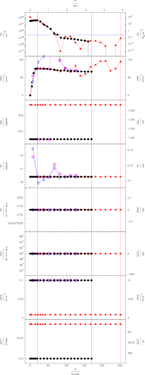
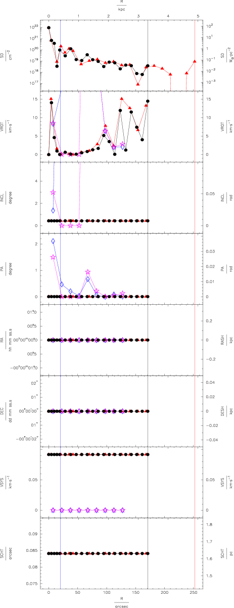
Quantity	Range	method	$N_{{H\textsc{i}}}$	$\frac{N_{{H\textsc{i}}}}{N_{{H\textsc{i}}},exp}$	$v_{\rm rot}$	$i$	$pa$	${\rm RA}$	${\rm DEC}$	$v_{\rm sys}$	$z_{0}$
(1)	(2)	(3)	(4)	(5)	(6)	(7)	(8)	(9)	(10)	(11)	(12)
$\overline{\Delta}$	all	tir	486.53	0.678	5.0	0.4	0.0	0.0	0.0	0.1	0.1
$\sqrt{\overline{\Delta^{2}}}$	all	tir	2020.45	1.118	7.6	0.4	0.0	0.0	0.0	0.1	0.1
$\Delta_{\rm max}$	all	tir	9446.95	2.810	15.1	0.4	0.0	0.0	0.0	0.1	0.1
$\overline{\Delta}$	70%	tir	4.54	0.198	1.5	0.4	0.0	0.0	0.0	0.1	0.1
$\sqrt{\overline{\Delta^{2}}}$	70%	tir	5.69	0.325	2.4	0.4	0.0	0.0	0.0	0.1	0.1
$\Delta_{\rm max}$	70%	tir	10.50	0.773	6.6	0.4	0.0	0.0	0.0	0.1	0.1
$\overline{\Delta}$	hi	tir	81.15	0.086	0.4	0.4	0.0	0.0	0.0	0.1	0.1
$\sqrt{\overline{\Delta^{2}}}$	hi	tir	107.39	0.115	0.6	0.4	0.0	0.0	0.0	0.1	0.1
$\Delta_{\rm max}$	hi	tir	208.61	0.242	1.0	0.4	0.0	0.0	0.0	0.1	0.1
$\overline{\Delta}$	$8-\sigma$	tir	4.89	0.951	7.7	0.4	0.0	0.0	0.0	0.1	0.1
$\sqrt{\overline{\Delta^{2}}}$	$8-\sigma$	tir	6.46	1.235	9.2	0.4	0.0	0.0	0.0	0.1	0.1
$\Delta_{\rm max}$	$8-\sigma$	tir	14.21	2.810	15.1	0.4	0.0	0.0	0.0	0.1	0.1
$\overline{\Delta}$	$2-\sigma$	tir	4.46	1.052	8.7	0.4	0.0	0.0	0.0	0.1	0.1
$\sqrt{\overline{\Delta^{2}}}$	$2-\sigma$	tir	6.04	1.317	9.9	0.4	0.0	0.0	0.0	0.1	0.1
$\Delta_{\rm max}$	$2-\sigma$	tir	14.21	2.810	15.1	0.4	0.0	0.0	0.0	0.1	0.1
$\overline{\Delta}$	$0.5-\sigma$	tir	3.65	1.062	9.6	0.4	0.0	0.0	0.0	0.1	0.1
$\sqrt{\overline{\Delta^{2}}}$	$0.5-\sigma$	tir	4.77	1.364	10.6	0.4	0.0	0.0	0.0	0.1	0.1
$\Delta_{\rm max}$	$0.5-\sigma$	tir	8.92	2.810	15.1	0.4	0.0	0.0	0.0	0.1	0.1
$\overline{\Delta}$	excs	tir	2.70
$\sqrt{\overline{\Delta^{2}}}$	excs	tir	4.06
$\Delta_{\rm max}$	excs	tir	8.92
$\overline{\Delta}$	all	pk			19.9	15.2	0.3	0.0	0.0	0.0
$\sqrt{\overline{\Delta^{2}}}$	all	pk			44.8	23.7	0.6	0.0	0.0	0.0
$\Delta_{\rm max}$	all	pk			131.0	56.5	1.5	0.0	0.0	0.0
$\overline{\Delta}$	70%	pk			1.9	4.4	0.0	0.0	0.0	0.0
$\sqrt{\overline{\Delta^{2}}}$	70%	pk			3.0	6.9	0.1	0.0	0.0	0.0
$\Delta_{\rm max}$	70%	pk			6.3	12.2	0.1	0.0	0.0	0.0
$\overline{\Delta}$	hi	pk			32.7	14.1	0.2	0.0	0.0	0.0
$\sqrt{\overline{\Delta^{2}}}$	hi	pk			65.5	28.3	0.5	0.0	0.0	0.0
$\Delta_{\rm max}$	hi	pk			131.0	56.5	0.9	0.0	0.0	0.0
$\overline{\Delta}$	all	m1			42.8	29.9	0.4	0.0	0.0	0.0
$\sqrt{\overline{\Delta^{2}}}$	all	m1			73.2	35.5	0.8	0.0	0.0	0.0
$\Delta_{\rm max}$	all	m1			93.9	61.8	2.1	0.0	0.0	0.0
$\overline{\Delta}$	70%	m1			10.9	19.4	0.1	0.0	0.0	0.0
$\sqrt{\overline{\Delta^{2}}}$	70%	m1			14.4	23.5	0.1	0.0	0.0	0.0
$\Delta_{\rm max}$	70%	m1			28.4	37.8	0.2	0.0	0.0	0.0
$\overline{\Delta}$	hi	m1			84.6	47.6	0.3	0.0	0.0	0.0
$\sqrt{\overline{\Delta^{2}}}$	hi	m1			108.7	48.6	0.4	0.0	0.0	0.0
$\Delta_{\rm max}$	hi	m1			192.3	61.8	0.7	0.0	0.0	0.0

Figure 22: Test 13: asymmetric warp with variable scale height, central shift and shift in systemic velocity. Noise added to the data cube. ROTCUR: optimal first guess. All parameters except expansion velocity were left variable. For symbol- and colour coding see the introduction to this section.

Table 14: Test 13: asymmetric warp with variable scale height, central shift and shift in systemic velocity. Noise added to the data cube. Deviation in global dispersion: 0.08 ${\rm km}\,{\rm s}^{-1}$. ROTCUR: optimal first guess. All parameters except expansion velocity were left variable.

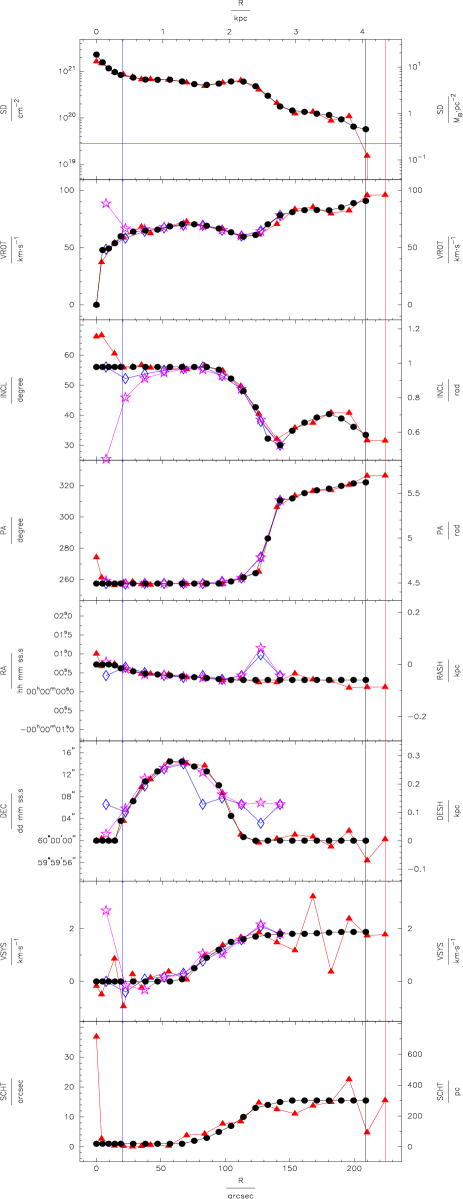
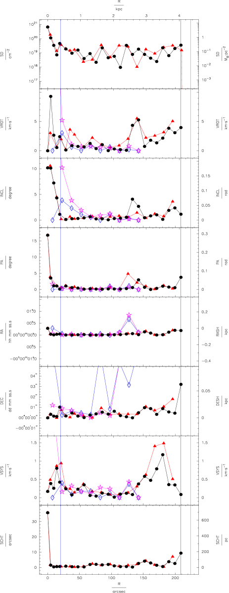
Quantity	Range	method	$N_{{H\textsc{i}}}$	$\frac{N_{{H\textsc{i}}}}{N_{{H\textsc{i}}},exp}$	$v_{\rm rot}$	$i$	$pa$	${\rm RA}$	${\rm DEC}$	$v_{\rm sys}$	$z_{0}$
(1)	(2)	(3)	(4)	(5)	(6)	(7)	(8)	(9)	(10)	(11)	(12)
$\overline{\Delta}$	all	tir	58.49	0.089	2.1	2.1	2.0	0.9	0.5	0.5	3.7
$\sqrt{\overline{\Delta^{2}}}$	all	tir	156.54	0.145	2.6	3.8	4.3	1.5	0.7	0.6	8.8
$\Delta_{\rm max}$	all	tir	667.63	0.442	5.5	10.6	16.8	4.3	1.8	1.5	35.9
$\overline{\Delta}$	70%	tir	12.31	0.029	1.3	0.5	0.5	0.3	0.2	0.2	1.0
$\sqrt{\overline{\Delta^{2}}}$	70%	tir	15.05	0.036	1.5	0.6	0.6	0.4	0.3	0.2	1.1
$\Delta_{\rm max}$	70%	tir	27.88	0.069	2.6	0.8	1.1	0.6	0.4	0.5	1.7
$\overline{\Delta}$	hi	tir	18.82	0.079	2.3	0.8	0.9	0.7	0.6	0.5	1.8
$\sqrt{\overline{\Delta^{2}}}$	hi	tir	22.50	0.137	2.8	1.2	1.5	1.1	0.7	0.6	2.5
$\Delta_{\rm max}$	hi	tir	36.76	0.442	5.5	3.6	4.9	3.1	1.8	1.5	7.1
$\overline{\Delta}$	$8-\sigma$	tir	16.76	0.215	3.3	1.5	0.7	1.5	1.2	1.0	3.4
$\sqrt{\overline{\Delta^{2}}}$	$8-\sigma$	tir	19.86	0.257	3.4	2.0	0.8	2.0	1.2	1.1	4.3
$\Delta_{\rm max}$	$8-\sigma$	tir	33.35	0.442	5.1	3.6	1.2	3.1	1.8	1.5	7.1
$\overline{\Delta}$	excs	tir	7.70
$\sqrt{\overline{\Delta^{2}}}$	excs	tir	10.89
$\Delta_{\rm max}$	excs	tir	15.40
$\overline{\Delta}$	all	pk			4.9	5.0	0.4	1.8	2.3	0.4
$\sqrt{\overline{\Delta^{2}}}$	all	pk			12.7	10.3	0.6	4.1	3.5	0.9
$\Delta_{\rm max}$	all	pk			39.7	30.7	1.7	12.6	6.9	2.7
$\overline{\Delta}$	70%	pk			0.5	0.7	0.1	0.3	0.6	0.1
$\sqrt{\overline{\Delta^{2}}}$	70%	pk			0.5	1.0	0.1	0.4	0.7	0.2
$\Delta_{\rm max}$	70%	pk			0.8	1.9	0.3	1.0	1.2	0.3
$\overline{\Delta}$	hi	pk			1.1	2.1	0.2	1.9	2.4	0.2
$\sqrt{\overline{\Delta^{2}}}$	hi	pk			1.8	3.7	0.4	4.3	3.7	0.2
$\Delta_{\rm max}$	hi	pk			5.2	10.2	0.8	12.6	6.9	0.4
$\overline{\Delta}$	all	m1			0.5	0.9	0.3	2.1	3.1	0.1
$\sqrt{\overline{\Delta^{2}}}$	all	m1			1.0	1.5	0.5	3.6	4.1	0.2
$\Delta_{\rm max}$	all	m1			3.0	3.9	1.1	10.0	6.6	0.4
$\overline{\Delta}$	70%	m1			0.1	0.3	0.0	0.6	1.6	0.1
$\sqrt{\overline{\Delta^{2}}}$	70%	m1			0.2	0.5	0.0	0.8	2.4	0.1
$\Delta_{\rm max}$	70%	m1			0.6	1.1	0.1	1.7	5.3	0.2
$\overline{\Delta}$	hi	m1			0.6	1.0	0.3	1.8	2.7	0.1
$\sqrt{\overline{\Delta^{2}}}$	hi	m1			1.1	1.6	0.5	3.4	3.7	0.2
$\Delta_{\rm max}$	hi	m1			3.0	3.9	1.1	10.0	6.6	0.4

Figure 23: Test 14: asymmetric warp with variable scale height, central shift and shift in systemic velocity. Noise added to the data cube. The cloud flux used was $10^{-3}\,{\rm Jy}\,{\rm km}\,{\rm s}^{-1}$ for a radius below $48\arcsec$, $10^{-4}\,{\rm Jy}\,{\rm km}\,{\rm s}^{-1}$ for a radius between $48\arcsec$ and $114\arcsec$, and $10^{-4}\,{\rm Jy}\,{\rm km}\,{\rm s}^{-1}$ beyond $114\arcsec$, correspinding to H i masses of $3.8\cdot 10^{4}\,{\rm M}_{\odot}$, $3.8\cdot 10^{3}\,{\rm M}_{\odot}$, and $3.8\cdot 10^{2}\,{\rm M}_{\odot}$, respectively, for a galaxy at a distance of $4\,{\rm Mpc}$, the cloud masses scaling with the distance squared. With this setup, an inhomogeneous distibution of the H i was simulated. Since the orientation of the galactic disk is near to edge-on, no attempt was made to perform a fit to the velocity field. For symbol- and colour coding see the introduction to this section.

Table 15: Test 14: asymmetric warp with variable scale height, central shift and shift in systemic velocity. Noise added to the data cube. The cloud flux used was $10^{-3}\,{\rm Jy}\,{\rm km}\,{\rm s}^{-1}$ for a radius below $48\arcsec$, $10^{-4}\,{\rm Jy}\,{\rm km}\,{\rm s}^{-1}$ for a radius between $48\arcsec$ and $114\arcsec$, and $10^{-4}\,{\rm Jy}\,{\rm km}\,{\rm s}^{-1}$ beyond $114\arcsec$, correspinding to H i masses of $3.8\cdot 10^{4}\,{\rm M}_{\odot}$, $3.8\cdot 10^{3}\,{\rm M}_{\odot}$, and $3.8\cdot 10^{2}\,{\rm M}_{\odot}$, respectively, for a galaxy at a distance of $4\,{\rm Mpc}$, the cloud masses scaling with the distance squared. With this setup, an inhomogeneous distibution of the H i was simulated. Since the orientation of the galactic disk is near to edge-on, no attempt was made to perform a fit to the velocity field.

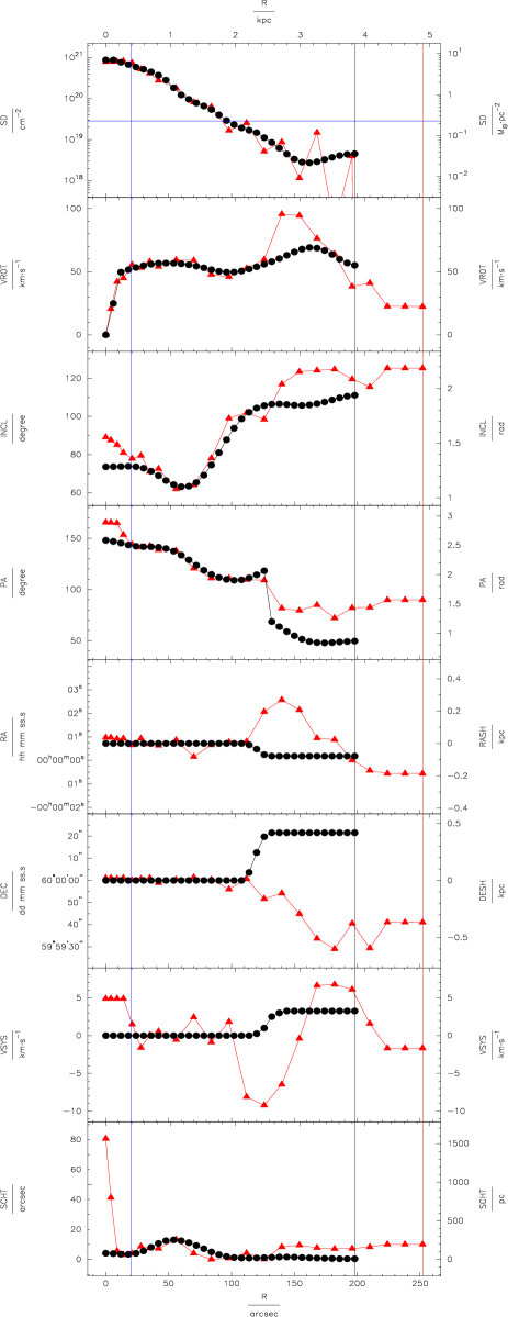
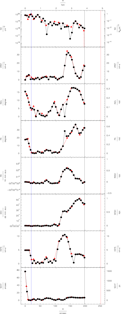
Quantity	Range	method	$N_{{H\textsc{i}}}$	$\frac{N_{{H\textsc{i}}}}{N_{{H\textsc{i}}},exp}$	$v_{\rm rot}$	$i$	$pa$	${\rm RA}$	${\rm DEC}$	$v_{\rm sys}$	$z_{0}$
(1)	(2)	(3)	(4)	(5)	(6)	(7)	(8)	(9)	(10)	(11)	(12)
$\overline{\Delta}$	all	tir	26.60	0.471	6.9	8.2	12.1	7.9	13.1	3.7	9.2
$\sqrt{\overline{\Delta^{2}}}$	all	tir	44.24	1.013	11.4	10.0	16.7	13.2	22.5	4.7	20.0
$\Delta_{\rm max}$	all	tir	110.27	4.126	34.4	17.5	36.9	35.9	52.6	10.2	76.4
$\overline{\Delta}$	70%	tir	5.88	0.130	2.6	5.0	5.5	2.1	1.1	2.1	2.5
$\sqrt{\overline{\Delta^{2}}}$	70%	tir	8.52	0.161	2.9	6.0	8.1	2.4	1.5	2.6	3.3
$\Delta_{\rm max}$	70%	tir	21.57	0.385	4.2	10.4	18.0	3.7	4.0	4.9	6.6
$\overline{\Delta}$	hi	tir	42.58	0.122	2.8	3.0	2.2	2.5	0.7	1.1	2.6
$\sqrt{\overline{\Delta^{2}}}$	hi	tir	58.27	0.142	3.0	3.5	2.6	3.6	0.9	1.3	3.4
$\Delta_{\rm max}$	hi	tir	110.27	0.252	4.2	6.4	4.7	8.4	1.4	2.4	5.8
$\overline{\Delta}$	$8-\sigma$	tir	4.10	0.795	10.5	9.1	16.0	12.9	24.1	4.6	5.1
$\sqrt{\overline{\Delta^{2}}}$	$8-\sigma$	tir	5.76	1.390	15.4	10.9	20.6	18.0	31.1	5.6	5.7
$\Delta_{\rm max}$	$8-\sigma$	tir	11.99	4.126	34.4	17.5	36.9	35.9	52.6	10.2	8.2
$\overline{\Delta}$	$2-\sigma$	tir	3.79	0.969	12.1	10.9	19.0	15.0	29.9	5.4	5.1
$\sqrt{\overline{\Delta^{2}}}$	$2-\sigma$	tir	5.61	1.554	17.0	12.1	22.9	19.9	34.7	6.2	5.8
$\Delta_{\rm max}$	$2-\sigma$	tir	11.99	4.126	34.4	17.5	36.9	35.9	52.6	10.2	8.2
$\overline{\Delta}$	$0.5-\sigma$	tir	2.36	1.279	17.7	13.9	28.0	18.0	41.1	4.6	7.1
$\sqrt{\overline{\Delta^{2}}}$	$0.5-\sigma$	tir	4.36	1.933	21.4	14.4	28.7	21.9	42.0	5.2	7.1
$\Delta_{\rm max}$	$0.5-\sigma$	tir	11.99	4.126	34.4	17.5	36.9	35.9	52.6	9.5	8.2
$\overline{\Delta}$	excs	tir	0.00
$\sqrt{\overline{\Delta^{2}}}$	excs	tir	0.00
$\Delta_{\rm max}$	excs	tir	0.00

Figure 24: Test 15: flat disk with constant scale height and solid-body rotation, no noise added to the data cube. While the fitting was in this case not performed without the knowledge of the parametrisation of the fake observation, convergence was reached very quickly: since TiRiFiC fits the surface brightness profile, the degeneracy of inclination and rotation velocity is broken. For symbol- and colour coding see the introduction to this section.

Table 16: Test 15: flat disk with constant scale height and solid-body rotation, no noise added to the data cube. Deviation in global dispersion: 0.01 ${\rm km}\,{\rm s}^{-1}$. While the fitting was in this case not performed without the knowledge of the parametrisation of the fake observation, convergence was reached very quickly: since TiRiFiC fits the surface brightness profile, the degeneracy of inclination and rotation velocity is broken.

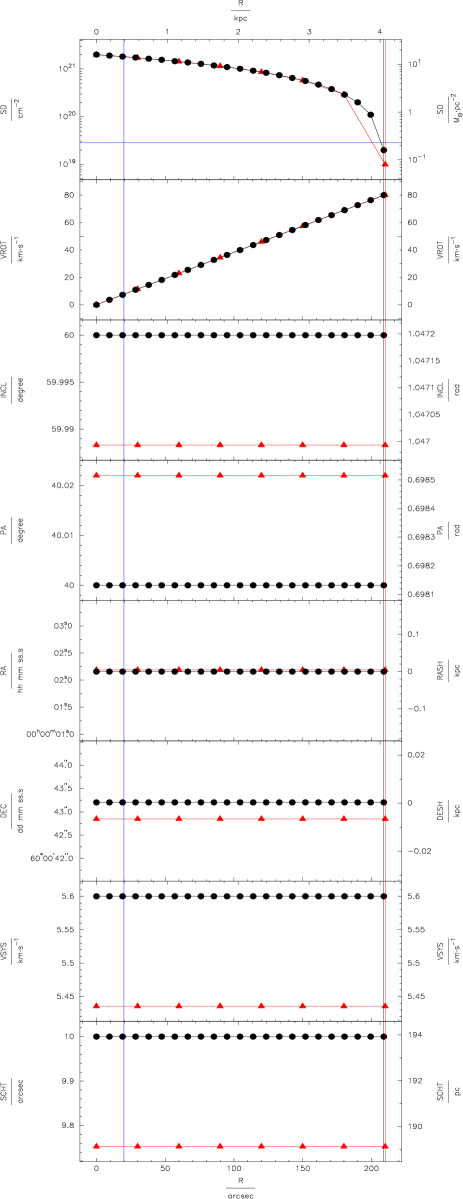
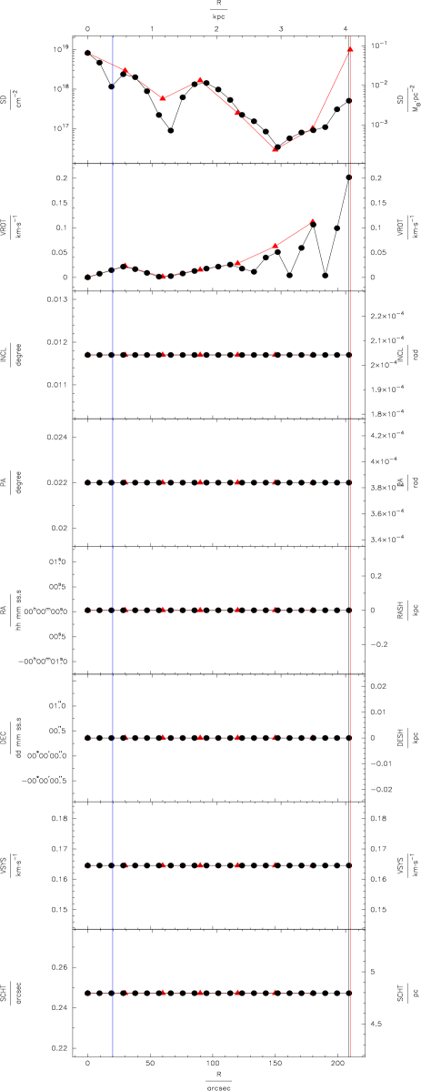
Quantity	Range	method	$N_{{H\textsc{i}}}$	$\frac{N_{{H\textsc{i}}}}{N_{{H\textsc{i}}},exp}$	$v_{\rm rot}$	$i$	$pa$	${\rm RA}$	${\rm DEC}$	$v_{\rm sys}$	$z_{0}$
(1)	(2)	(3)	(4)	(5)	(6)	(7)	(8)	(9)	(10)	(11)	(12)
$\overline{\Delta}$	all	tir	2.98	0.001	0.0	0.0	0.0	0.5	0.4	0.2	0.2
$\sqrt{\overline{\Delta^{2}}}$	all	tir	4.74	0.002	0.1	0.0	0.0	0.5	0.4	0.2	0.2
$\Delta_{\rm max}$	all	tir	9.99	0.004	0.1	0.0	0.0	0.5	0.4	0.2	0.2
$\overline{\Delta}$	70%	tir	0.52	0.000	0.0	0.0	0.0	0.5	0.4	0.2	0.2
$\sqrt{\overline{\Delta^{2}}}$	70%	tir	0.80	0.000	0.0	0.0	0.0	0.5	0.4	0.2	0.2
$\Delta_{\rm max}$	70%	tir	1.67	0.000	0.0	0.0	0.0	0.5	0.4	0.2	0.2
$\overline{\Delta}$	hi	tir	0.93	0.001	0.0	0.0	0.0	0.5	0.4	0.2	0.2
$\sqrt{\overline{\Delta^{2}}}$	hi	tir	1.41	0.001	0.1	0.0	0.0	0.5	0.4	0.2	0.2
$\Delta_{\rm max}$	hi	tir	2.95	0.002	0.1	0.0	0.0	0.5	0.4	0.2	0.2
$\overline{\Delta}$	excs	tir	9.99
$\sqrt{\overline{\Delta^{2}}}$	excs	tir	9.99
$\Delta_{\rm max}$	excs	tir	9.99