Image Ellipticity from Atmospheric Aberrations

Abstract

We investigate the ellipticity of the point-spread function (PSF) produced by imaging an unresolved source with a telescope, subject to the effects of atmospheric turbulence. It is important to quantify these effects in order to understand the errors in shape measurements of astronomical objects, such as those used to study weak gravitational lensing of field galaxies. The PSF modeling involves either a Fourier transform of the phase information in the pupil plane or a ray-tracing approach, which has the advantage of requiring fewer computations than the Fourier transform. Using a standard method, involving the Gaussian weighted second moments of intensity, we then calculate the ellipticity of the PSF patterns. We find significant ellipticity for the instantaneous patterns (up to more than 10%). Longer exposures, which we approximate by combining multiple ($N$) images from uncorrelated atmospheric realizations, yield progressively lower ellipticity (as $1/\sqrt{N}$). We also verify that the measured ellipticity does not depend on the sampling interval in the pupil plane using the Fourier method. However, we find that the results using the ray-tracing technique do depend on the pupil sampling interval, representing a gradual breakdown of the geometric approximation at high spatial frequencies. Therefore, ray tracing is generally not an accurate method of modeling PSF ellipticity induced by atmospheric turbulence unless some additional procedure is implemented to correctly account for the effects of high spatial frequency aberrations. The Fourier method, however, can be used directly to accurately model PSF ellipticity, which can give insights into errors in the statistics of field galaxy shapes used in studies of weak gravitational lensing.

1 Introduction

Statistical analyses of weak gravitational lensing of field galaxies (e.g., Wittman et al., 2000; Van Waerbeke et al., 2000; Bacon et al., 2000) are being used as probes of cosmology and are expected to provide some of the strongest cosmological tests in future, large astronomical survey projects, such as the Large Synoptic Survey Telescope (LSST; e.g., Tyson & Angel, 2001; Tyson, 2002). These surveys will allow for the precise determination of various cosmological parameters, such as the matter density distribution $\Omega_{m}$, the cosmological constant $\Omega_{\Lambda}$, the equation of state $w$ of the dark energy, and its time derivative. This is done by accurately analyzing large numbers of background galaxies as their shapes are sheared by intervening large-scale structure through weak gravitational lensing, the results of which are then combined with, e.g., the very accurate measurements of the cosmic microwave background radiation by the WMAP satellite.

A critical part in these analyses is the accuracy to which one can measure and correct the shape of the Point Spread Function (PSF) as it varies across the detector (see, e.g., Hoekstra, 2004). This PSF anisotropy is largely induced by the atmosphere (e.g., Wittman, 2005), and cannot easily be modeled without incorporating an explicit atmosphere. It is possible to mimic the effects of the atmosphere by convolving either artificially generated, or high resolution HST images with a suitable PSF (see, e.g., Heymans et al. 2006a for the former, and Bacon et al. 2001 for the latter approach), but that still does not include effects of PSF anisotropy. We therefore set out to model the behavior of the PSF as it gets folded through a realistic atmosphere and telescope system. Since ray-tracing methods are commonly used to simulate the shearing signal of weak lensing by large scale structure (e.g., Jain et al., 2000; Vale & White, 2003; Heymans et al., 2006b), we include both ray-tracing and Fourier transform methods to calculate what the PSF should be based on the phase and intensity information in the pupil plane of the telescope. The ray-tracing method has the advantage of computational speed compared with the Fourier transform method. However, the Fourier transform method correctly treats the effects of interference, which are ignored by the geometric ray-tracing method. Because of its relative computational efficiency, it is useful to understand whether the ray tracing approach gives adequate PSF ellipticity information. More importantly, it is crucial to understand the elliptical properties of the PSF in order to enable quantitative analysis of the errors in statistical studies of field galaxy shapes.

Our modeled observational setup is characterized as follows: a generic 8 m-class telescope, a turbulent atmosphere with a Kolmogorov power spectrum, and a single, on-axis point-source located at infinity. The ellipticity and its direction are assumed to be representative for a single region over which these quantities do not vary. The angular extent of these regions can be, depending on observing conditions, larger than an arcminute (e.g., Asztalos et al., 2006). Since the typical LSST exposure will be 15 seconds, we also investigate the time dependence of the atmospherically induced ellipticities, and how it imposes limits on the ability to measure them.

1.1 Layout of the paper

The paper is organized as follows. In § 2 and § 3, we discuss the atmospheric simulations and the methods applied to calculate the PSF ellipticity. Then in § 4, we describe the results for both the ray-tracing method (RTM) and the Fourier transform method (FTM). The main difference between these two is the way one models image formation by the telescope. The RTM traces the geometric path of rays from the pupil plane onto the focal plane, whereas the FTM applies a Fourier transform to the complex electromagnetic field in the pupil plane in order to calculate the resulting image. The latter correctly incorporates effects of interference, unlike the RTM. The geometric approximation of the RTM has implications for shape measurements in the image plane, which we quantify in this paper.

The results are subdivided into the effects of pupil plane sampling (§ 4.1), the variation of ellipticity as a function of exposure time and the presence of wind (§ 4.3), and seeing (§ 4.4). The latter is approximated by using varying ratios of D / r_o (where D is the aperture size of the telescope, and r_o is the coherence length of the atmosphere). Longer exposure times are simulated by increasing the number of completely independent phase screens (which is a function of aperture diameter and wind-speed). In order to check the accuracy of this approximation, we also evaluate a model that includes intermediate phase screens, i.e., screens that are not completely decorrelated from the previous one, but are translated by a small fraction of the aperture size along the wind direction. In each of these sections we investigate the differences between the RTM and FTM, which are summarized in § 5.

2 Simulations and Methods

We generated random phases for the electromagnetic field in the pupil of the telescope using Kolmogorov statistics to represent the effects of atmospheric turbulence. The inner turbulence scale of the simulations is set by the pixel size used in the simulations, to a fraction of r_o . The outer scale of the turbulence has been fixed to a value larger than the simulation box ($>800$ m for the large screens in § 4.3, for instance), so that effectively the simulations see a Kolmogorov turbulence spectrum with an infinite outer scale. Assuming a constant magnitude in the circular pupil, we propagated the field to the focal plane using a Fourier transform, and by squaring the resulting magnitude, created a representation of the focal plane image intensity. These images contain distinct speckle patterns for different realizations of the atmosphere.

The ray tracing algorithm used an idealized model of a reflecting telescope. A Kolmogorov phase screen was placed in the aperture of the telescope and a uniform distribution of rays in the pupil was assumed. The $x$ and $y$ derivatives of the phase screen were used to determine the atmospherically induced deviations of the rays as they propagated toward the focus of the telescope. At the focus, the incoming rays are mapped onto a fiducial 2D detector grid which determines the intensity distribution in the focal plane.

3 Calculating Ellipticity

Figure 1: Representative point-spread functions, using the Fourier method (left two images), and the ray-tracing method (right two images). The top images are for an instantaneous realization of the atmosphere, whereas the bottom images are the means for 256 such instances. Notice that the top left Fourier image displays a prominent speckle pattern due to interference. This pattern gets washed out over time.

We calculate the ellipticity of an object in the pupil plane as follows. Assume we have an image for which the pixel coordinates are given by $x=1..N,y=1..N$; the intensity in each pixel is given by $I(x,y)$; the seeing is given by $\sigma$ (FWHM=2.355$\sigma$ for a Gaussian), and the central point source is located at $(x_{c},y_{c})$. We then define Gaussian weights as follows:

$$w(x,y)=\frac{1}{\sqrt{(2\pi\sigma^{2})}}e^{-\frac{1}{2\sigma^{2}}(x-x_{c})^{2}}.\frac{1}{\sqrt{(2\pi\sigma^{2})}}e^{-\frac{1}{2\sigma^{2}}(y-y_{c})^{2}}$$ (1)

and the Gaussian weighted moments:

$$S_{w}=\sum_{x,y=1}^{N}(I(x,y)w(x,y)),\,S_{xx}=\sum_{x,y=1}^{N}(x^{2}I(x,y)w(x,y))$$

$$S_{x}=\sum_{x,y=1}^{N}(xI(x,y)w(x,y)),\,S_{yy}=\sum_{x,y=1}^{N}(y^{2}I(x,y)w(x,y))$$

$$S_{y}=\sum_{x,y=1}^{N}(yI(x,y)w(x,y)),\,S_{xy}=\sum_{x,y=1}^{N}(xyI(x,y)w(x,y))$$

This allows us to define the following quantities (all weighted by $I(x,y)w(x,y)$):

$$x_{c}=S_{x}/S_{w},\quad y_{c}=S_{y}/S_{w}$$

$$\left(\begin{array}[]{c}rxx\\ ryy\\ rxy\end{array}\right)=\left(\frac{1}{S_{w}S_{w}}\right)\left(\begin{array}[]{c}S_{xx}S_{w}-S_{x}S_{x}\\ S_{yy}S_{w}-S_{y}S_{y}\\ S_{xy}S_{w}-S_{x}S_{y}\end{array}\right)$$ (9)

From these, one can calculate the image Gaussian scale length $\sigma$ and the ellipticity $\epsilon$:

$$\sigma=\sqrt{rxx+ryy}$$

$$\epsilon=\left(\frac{((rxx-ryy)^{2}+(2rxy)^{2}}{(rxx+ryy)^{2}}\right)^{1/2}$$

$$\epsilon_{1}=\frac{rxx-ryy}{rxx+ryy},\quad\epsilon_{2}=\frac{2rxy}{rxx+ryy}$$ (10)

This is the method used by Kaiser, Squires, & Broadhurst (1995, KSB) - see also Heymans et al. (2006a) for an overview of the different weak lensing pipelines. The weights in eqn. 1 are dependent on initial values of $\sigma$, and the source centroid $(x_{c},y_{c})$. However, one can iterate from initial guesses for the unknowns. This algorithm converges quickly (typically within a few steps), and yields values for $\sigma$ and the source position that are readily verifiable. We terminate the iterations when the changes in $\sigma$ are less than 0.01 pixel.

4 Results

Figure 2: Ellipticity as function of the number of independent phase screens and sampling rates for D / r_o = 40 (r_o = 21cm). The left panel shows the results for ray-tracing, with the pupil-plane sampling rates color-coded as: r_o / 2 green, r_o / 4 blue, r_o / 5 cyan, r_o / 8 purple, and r_o / 16 yellow. The panel on the right shows the same results (except r_o / 5) for the Fourier method. The latter method clearly illustrates the expected behavior: ellipticity should be independent of pupil plane sampling rates beyond Nyquist rates. The progressive lowering of the curves for higher samping rates in the left panel, therefore, is unphysical. The dashed line in the right panel shows a $1/\sqrt{N}$ decline.

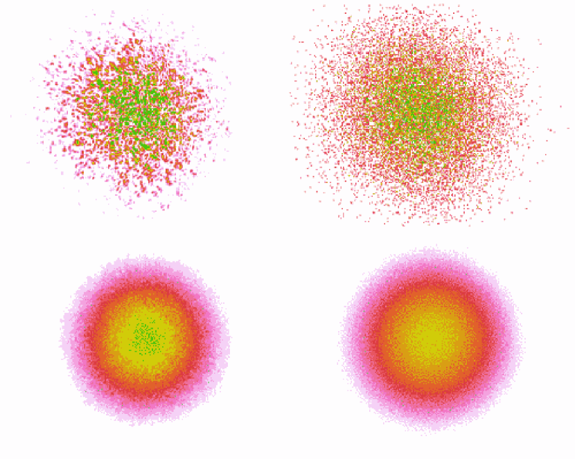
Most of the figures in this paper show the ellipticity behavior as a function of the number $N$ of independent phase screens. A single phase screen ($N=1$) therefore represents the instantaneous ellipticity of a particular representation of the atmosphere (see Fig. 1). In all of our subsequent discussions we assume that the telescope is perfect, i.e., it does not induce image aberrations.

Whether we apply the RTM or the FTM approach, we first create stacks of 500 completely uncorrelated instances of the atmosphere (actually phase-screens in the pupil plane). The resulting focal plane images are then either ray-traced or calculated using an appropriate Fourier transform. After this, we randomly select $N$ frames out of the 500, which are then stacked, averaged, and have their ellipticity calculated. We repeat this $1024/N$ times. Since there are not $1024/N$ fully independent stacks present (for $N>2$), some smoothing occurs, especially for the larger $N$ stacks. The figures show the mean ellipticity for these $1024/N$ stacks, and the error-bars on the means are approximated by the rms of the distribution divided by the square root of the number of stacks ($1024/N$).

4.1 Constant ratio D / r_o , varying sampling in pupil plane

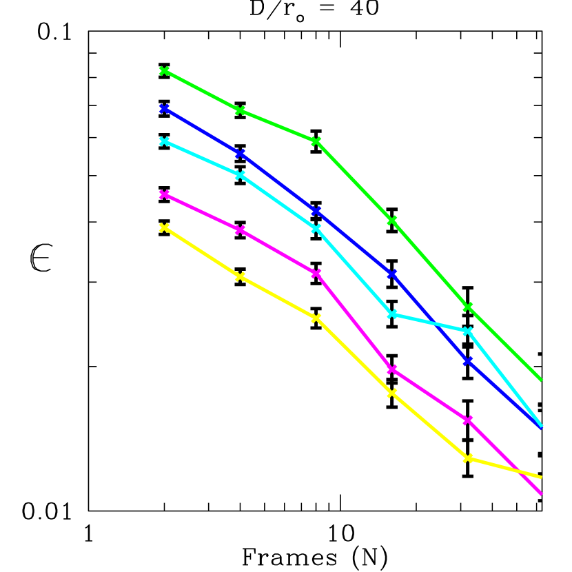
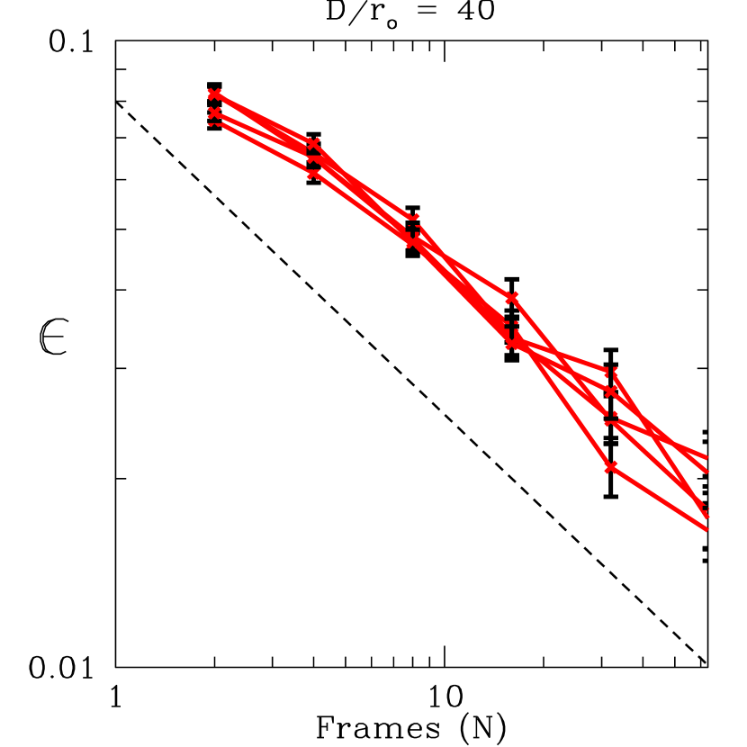
The value of D / r_o has been fixed at 40 (r_o = 21 cm) for an assumed 8.4 m pupil diameter with a central obscuration of 5.4 m, while the (phase) sampling rate in the pupil plane increases from r_o / 2 to r_o / 16. The ellipticity $\epsilon$ as function of the number of independent phase screens $N$ is shown in Fig. 2. The left panel illustrates the results for the RTM method. While each individual sampling rate falls off as $1/\sqrt{N}$, they are offset in ellipticity as the sampling rate increases. An increase from r_o / 2 to r_o / 16 more than halves the measured ellipticity for a given number of independent phase screens. This is clearly not physical.

The following example may illuminate this behavior. Assume, for instance, a simple one-dimensional cosine phase wave with frequency $k$. The Fourier transform of this function produces two delta functions located at $\pm k$ on the x-axis. However, since ray-tracing uses the derivatives of the phase to calculate where the rays will go, it produces a spread of points due to the range in derivatives. An increase in the sampling rate will increase the likelihood high angle rays will be modeled. Furthermore, the derivative range becomes larger for higher spatial frequencies (it goes from $-k$ to $+k$) resulting in progressively more aberrant rays, regardless of the sampling rate. While perhaps an extreme example, it does underline the fact that 2D ray-tracing will produce a more spread-out image due to rays being deflected into unphysical angles. This broadening of the image then results in a lowered ellipticity as it decreases the local asymmetry (remember that the ellipticity contribution of a point is weighted by its distance, see Eqn. 1).

The FTM, on the other hand, does display the correct behavior (for the exact same sets of phase screens): the ellipticity is independent of the sampling rate (provided it is at least r_o / 2). Except for the sampling dependency, both methods exhibit the following characteristics. First, ellipticities decrease linearly (in log-log) as the number of frames increases. The slope is consistent with a $1/\sqrt{N}$ decline ($\alpha=-0.5$), as indicated by the dashed line in the right panel. And second, ellipticities of individual speckle images ($N=1$) are $\sim$9% for D / r_o = 40 (r_o = 21 cm).

It should also be noted that there are $\sim 20-40$ independent instances of the atmosphere for an 8.4 meter telescope aperture with wind-speeds of $\sim 10-20$ m/s (typical, turbulence-weighted values for many astronomical sites) and a 15 second exposure. Therefore, these simulations predict that the raw ellipticity of a 15-second exposure for a point source image through an 8.4 meter telescope with D / r_o = 40 is $\sim 2$%. We explore the effects of wind in more detail in § 4.3.

4.2 Binning in the image plane

Obviously, no astronomical instrument designed for seeing-limited observations will sample the PSF at the Nyquist interval for the telescope diffraction pattern (we measure $\sigma\sim 60$ pixels), so the next step is to see what happens to the ellipticities if one progressively rebins the images of Fig. 1. The results are listed in Table 1. The ellipticities are for a stack of 32 random frames with D / r_o = 40. This stack gets increasingly rebinned down to scales where the PSF is barely resolved ($\sigma\sim 1$).

Given that the values of $\epsilon$ do not change significantly over a large range of binning, it is clear that the ellipticity measurements are robust and do not depend on the pixel scale. For comparison, the rms spread in the value of $\epsilon$ for distinct random stacks of 32 images is about 60% of the mean value of $\epsilon$, whereas the listed relative range in column 3 is only $\sim 5\%$ under rebinning.

Table 1: Pixel binning effects on ellipticity

Binning $n$	$\sigma_{n}$ [pix]	$\epsilon_{n}$	Ratio $\epsilon_{n}/\epsilon_{1}$ [%]
1	61.82	0.02505
2	30.92	0.02507	100.1
4	15.47	0.02504	100.0
8	7.74	0.02513	100.3
16	3.89	0.02492	99.5
32	1.97	0.02393	95.5
64	1.04	0.02443	97.5

Note. — The ellipticity is calculated on a random stack of 32 speckle patterns, with a sampling of r_o / 2, and a ratio of D / r_o = 40 (r_o = 21 cm). There is no significant dependency on pixel size. Note that $\sigma\sim 1$ to $2$ are typical astronomical seeing disk sampling ratios.

4.3 Atmospheric model with wind

Figure 3: Effect of wind on ellipticity behavior for D / r_o = 40 (r_o = 21 cm). The blue dashed curve is for phase screens which are translated across the aperture, and the red curve is for independent instances of the atmosphere. Both these curves are calculated with the Fourier method. The wind-speed $v$ is needed to convert the number of frames $N$ into an elapsed time $t$ ($=ND/v$, with $D$ = 8.4 m, and $v$ in units of m s^-1). Therefore, a typical 15 s LSST exposure, with a wind-speed of 10 m s^-1, contains 18 frames.

So far we have only considered the behavior of ellipticity as function of the number of uncorrelated instances of the atmosphere. As described in § 4.1, the evolution of the PSF with increasing exposure time can be estimated using the results from these uncorrelated screens by associating each screen with a unit of time equal to the aperture diameter divided by the wind speed, i.e., the time it would take for the wind to translate a screen completely out of the aperture. However, a more realistic treatment of the PSF evolution involves a more continuous translation of a Kolmogorov phase screen across the telescope aperture.

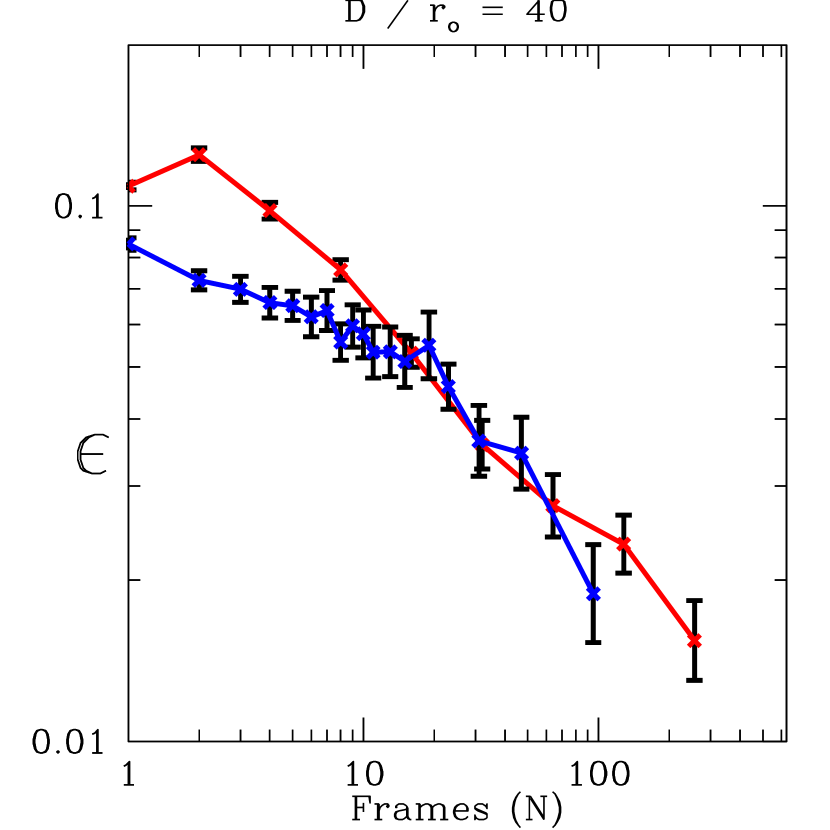
For this purpose, we generated 3 large phase screens which contain 95 aperture-clearings each. The translation offset is such that an aperture-clearing takes 20 steps; from each phase screen we therefore generate 1900 pupil images using the FTM. The ellipticity is then calculated on combined stacks of 20 pupil images, yielding one value per aperture-clearing. The results are plotted in Fig. 3. The blue dashed line shows the mean ellipticity values for all $3\times 95/N$ independent aperture-clearings (“frames”), with as error-bars the error in this mean. At $N=5$, for instance, we calculated the mean of all uncorrelated instances of $5\times 20$ consecutive pupil images. On the other hand, the red curve shows the ellipticity behavior of the sum of $N$ uncorrelated instances of the atmosphere, using the same pupil plane sampling and value of D / r_o = 40 (r_o = 21 cm).

A few things stand out. Below about 10 frames or so, the curves behave differently. In case of the red line, the ellipticity jump from $N=1$ to $N=2$ is due to the fact that there is no “image motion” in the $N=1$ case, whereas for $N=2$, two pupil images have been combined with different PSF centroids. This raises the ellipticity beyond what is there in a single PSF (one would need to shift-and-add to remove this effect). It subsequently takes a few more co-added frames for this centroid-offset effect to cancel out (on average the PSF has to align with the optical axis since we put the source there).

The blue line does not suffer from this centroid-offset problem since the phase-screens are continuous (only 1/20^th gets shifted out between pupil images) and the PSF centroid cannot move around discontinuous as a consequence. However, we do see another effect present in the blue curve. Because the Kolmogorov phase screen will generally have low-spatial-frequency correlations that are larger than the telescope aperture, the ellipticity of the PSF is expected to decrease more slowly with increasing $N$ than for the discontinuous model using multiple independent phase screens. After some time (or equivalently, for larger values of $N$), these low-spatial-frequency correlations disappear and the slope of the blue curve steepens to that of the red curve. This appears to be happening between $N=10$ and $N=20$.

The main result of this exercise, however, is the confirmation that our method of using uncorrelated instances timed at a rate equal to an aperture clearing time is a valid approximation for the ellipticity behavior in a statistical sense, as long as we are in the long-exposure, $N>20$ domain.

4.4 Varying r_o 

Figure 4: Speckle patterns for individual phase screens at various ratios of D / r_o (r_o = 21, 42, and 84 cm, respectively). Note that with increasing values of r_o (left to right), the number of speckles decreases, while their intensities go up. Also, the size of the pattern decreases with increasing r_o .

We also investigated the effect of increasing the value of r_o . The expectation is that for larger values of r_o (i.e., better seeing conditions) the number of speckles goes down (no atmosphere = no speckles, diffraction pattern only) while their individual brightness goes up (due to the conservation of flux). This is easily verified in the individual speckle patterns (see Fig. 4). It is not clear, however, what the behavior of the RTM method with respect to the FTM will be. In § 4.1, we noticed that the RTM method significantly underestimates the actual ellipticity depending on the sampling rate. If the relative offsets are constant then one might be able to come up with a particular sampling rate for the ray-tracing case that best matches the actual ellipticities (for the D / r_o = 40 case the best matching sampling looks to be about r_o / 3, see Fig. 2).

The results are presented in Fig. 5, with the solid lines representing the FTM results, and the dashed lines are for the RTM method. If we focus on the solid lines first, it is clear that the ellipticities increase with increasing values of r_o at the same number of stacked frames. This can be qualitatively understood in terms of the decreasing number of speckles distributing themselves in a progressively less circular pattern due to the smaller number statistics.

Figure 5: Measured ellipticities $\epsilon$ (see eqn. 4) for different values of r_o , with values from top to bottom of 42 (red, D / r_o =20), 21 (green, D / r_o = 40), and 10.5 cm (blue, D / r_o = 80), respectively. The solid line curves have been calculated using the Fourier method, and have a fixed pupil plane sampling rate of r_o / 4. The dashed lines are calculated using ray-tracing, and are color-coded and sampled similarly. The ellipticity for a given number of independent phase screens depends on the size of r_o : large values of r_o have larger ellipticities. Also note that low number statistics are affecting the data-points toward large frame counts causing the curves to cross eachother.

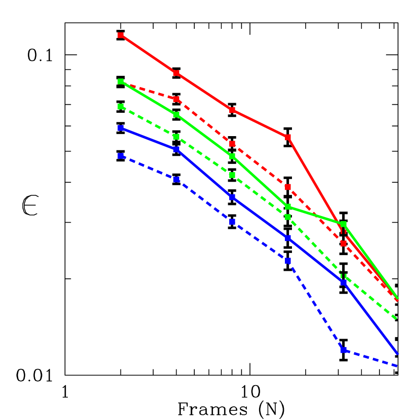
Based on this plot, it is also apparent that, even though the RTM underestimates the ellipticity compared to the FTM, it does so more or less independently of the value of r_o (which is a proxy for seeing). This might open up the possibility that one either selects a computationally efficient RTM sampling rate (say, r_o / 2) and apply an appropriate (fixed) correction factor to the ellipticity results, or adjust the sampling rate such that the RTM and FTM results are in good agreement ($\sim$r_o / 3). Another approach that is under investigation (G. Jernigan, private communication) is to roll off the atmospheric power spectra at high spatial frequencies. Further study is needed to assess the accuracy of any of these approaches. For instance, the numerical correction factors derived from the results shown in Fig. 5, for the particular sampling ratio of r_o / 4, are 1.32, 1.15, and 1.21, for r_o = 42 cm, r_o = 21 cm, and r_o = 10.5 cm, respectively. Whether this variation is due solely to the statistical errors in our modeling, or includes a systematic dependence on r_o is not known. Clearly if one requires accurate modeled ellipticities, then the computationally more expensive FTM is currently preferred.

5 Conclusions

Based on this analysis, we reach the following conclusions:

1. Instantaneous speckle patterns have ellipticities of $\sim$10% for D / r_o = 40 (r_o = 21 cm).

2. Co-adding multiple patterns results in a linearly decreasing ellipticity (on a log-log plot), consistent with a $\sqrt{N}$ slope of $\alpha=-0.5$.

3. Modeling phase screen transport across the aperture (i.e., wind) does not change the ellipticity results obtained from adding uncorrelated phase screens in the limit of long exposures ($N>20$ aperture clearings).

4. Ellipticity values are robust over a large range of pixel binning.

5. We expect no ellipticity dependency on sampling density in the pupil plane (above sampling of r_o / 2). This is confirmed for the Fourier method, but not for ray-tracing. The latter has a strong dependency on sampling rate, in the sense that the higher the sampling rate, the lower the resulting ellipticity. This can be understood as the result of a breakdown in the geometric approximation for high spatial frequency aberrations.

6. Ellipticities grow (for a given $N$) as the value of r_o increases. However, since the average size of the PSF goes down as r_o increases (see Fig. 4), the ability to measure precise ellipticities actually improves (for a given resolved object).

In summary, the effects of interference must be included in order to comprehensively model point-source ellipticities induced by the atmosphere. Therefore, care has to be taken that the geometric optics approximation to image formation by the telescope (i.e., ray tracing) produces the same modeling results, as this is not true in general.

References

- Asztalos et al. (2006) Asztalos, S., de Vries, W., Rosenberg, L. J., Treadway, T., Burke, D., Claver, C., Saha, A., & Puxley, P. 2007, ApJ, 659, 1
- Bacon et al. (2000) Bacon, D. J., Refregier, A. R., & Ellis, R. S. 2000, MNRAS, 318, 625
- Bacon et al. (2001) Bacon, D. J., Refregier, A. R., Clowe, D., & Ellis, R. S. 2001, MNRAS, 325, 1065
- Heymans et al. (2006a) Heymans, C., Van Waerbeke, L., Bacon, D., et al. 2006, MNRAS, 368, 1323
- Heymans et al. (2006b) Heymans, C., White, M., Heavens, A., Vale, C., & Van Waerbeke, L. 2006, MNRAS, in press (astro-ph/0604001)
- Hoekstra (2004) Hoekstra, H. 2004, MNRAS, 347, 1337
- Jain et al. (2000) Jain, B., Seljak, U., & White, S. 2000, ApJ, 530, 547
- Kaiser, Squires, & Broadhurst (1995) Kaiser, N., Squires, G., & Broadhurst, T. 1995, ApJ, 449, 460
- Tyson & Angel (2001) Tyson, A., & Angel, R. 2001, “The New Era of Wide Field Astronomy”, ASP conference series, Vol. 232, R. G. Clowes, A. J. Adamson, & G. E. Bromage, eds, p347
- Tyson (2002) Tyson, J. A., “Survey and Other Telescope Technologies and Discoveries”, Proceedings of the SPIE, Tyson, J. Anthony; Wolff, Sidney., eds, Vol. 4836, p10
- Vale & White (2003) Vale, C., & White, M. 2003, ApJ, 592, 699
- Van Waerbeke et al. (2000) Van Waerbeke, L., Mellier, Y., Erben, T., et al. 2000, A&A, 358, 30
- Wittman et al. (2000) Wittman, D. M.,Tyson, J. A., Kirkman, D., Dell’Antonio, I., & Bernstein, G. 2000, Nature, 405, 143
- Wittman (2005) Wittman, D. 2005, ApJ, 632, L5