Forecasting the Bayes factor of a future observation

Abstract

I present a new procedure to forecast the Bayes factor of a future observation by computing the Predictive Posterior Odds Distribution (PPOD). This can assess the power of future experiments to answer model selection questions and the probability of the outcome, and can be helpful in the context of experiment design.

As an illustration, I consider a central quantity for our understanding of the cosmological concordance model, namely the scalar spectral index of primordial perturbations, $n_{S}$. I show that the Planck satellite has over $90\%$ probability of gathering strong evidence against $n_{S}=1$, thus conclusively disproving a scale–invariant spectrum. This result is robust with respect to a wide range of choices for the prior on $n_{S}$.

1 Introduction

Many interesting questions in cosmology are not about parameter estimation, but rather about model selection. For example, we might be interested in assessing whether a new parameter is needed in our model, or whether a theoretical prediction for the value of a parameter can be confirmed by data.

These kind of questions often cannot be satisfactorily answered in the context of frequentist (sampling theory) statistics, but find their natural formulation in the framework of Bayesian model selection (see Trotta (2007c); Liddle (2007) and references therein). Bayesian model selection aims at working out the support that the data can offer to a model, by balancing the quality of fit that a more complicated model usually delivers with a quantitative embodiment of Occam’s razor, favouring simpler explanations whenever they are compatible with the observations at hand. This is usually expressed in terms of the Bayes factor between two competing models, which represents the amount by which our relative believe in the two model has changed after the arrival of the data. There is a growing body of work in cosmology and astrophysics applying various brands of model selection tools to a broad range of questions, see e.g. Drell et al. (2000); Loredo & Lamb (2002); Hobson & McLachlan (2003); Slosar et al. (2003); Saini et al. (2004); Lazarides et al. (2004); Beltran et al. (2005); Kunz et al. (2006); Marshall et al. (2006); Magueijo & Sorkin (2007); Parkinson et al. (2006); Trotta (2007a, b); Bevis et al. (2007).

The purpose of this paper is to present a new method to forecast the probability distribution of the Bayes factor for a future observation, called PPOD (for “Predictive Posterior Odds Distribution”).

Posterior odds forecasting was first introduced in Trotta (2005), which used a single model to describe the present data. This has inspired further developments of a similar technique in Pahud et al. (2006, 2007). In particular, Pahud et al. (2006) pointed out that the Bayes factor forecasting ought to consider multiple models and average over them. This approach is used in the present work. For a different approach to Bayes factor forecasting, see Mukherjee et al. (2006), which instead focuses on delineating regions of parameter space where future observations have the ability of delivering high–odds model selection results.

The use of our PPOD technique is illustrated on a central parameter of the cosmological concordance model, namely the scalar spectral index for cosmological perturbations, $n_{S}$, which can be related to the characteristics of the inflationary potential (see e.g. Leach & Liddle (2003)). One interesting question bears on whether the distribution of fluctuations is scale–invariant, i.e. whether a model with $n_{S}=1$ (the so-called Harrison-Zeldovich power spectrum) is supported by data. Current cosmological observations support the view that $n_{S}\neq 1$, with odds of about $17:1$ (Trotta, 2007c) (see also Pahud et al. (2006), who find odds of $8:1$ in favour of $n_{S}\neq 1$). In this paper, we derive a predictive distribution for $n_{S}$ for the Planck satellite – an European cosmic microwave background satellite due for launch next year – and present a forecast for the model selection outcome from Planck observations.

This paper is organized as follows: in section 2 we briefly review the main concepts of Bayesian model comparison. We then introduce our PPOD technique in section 3 and we apply it to derive the probability distribution for the model selection outcome from Planck in section 4, also discussing the dependence on the choice of prior. Section 5 is devoted to presenting our conclusions.

2 Bayesian model comparison

In this section we briefly review Bayesian model comparison and introduce our notation.

Bayesian inference (see e.g. Jaynes (2003); MacKay (2003)) is based on Bayes’ theorem, which is a consequence of the product rule of probability theory:

$$p({\theta}|{d},{M})=\frac{p({d}|{\theta},{M})\pi({\theta}|{M})}{p({d}|{M})}.$$ (1)

On the left-hand side, the posterior probability for the parameters ${\theta}$ given the data ${d}$ under a model ${M}$ is proportional to the likelihood $p({d}|{\theta},{M})$ times the prior probability distribution function (pdf), $\pi({\theta}|{M})$, which encodes our state of knowledge before seeing the data. In the context of model comparison it is more useful to think of $\pi({\theta}|{M}$) as an integral part of the model specification, defining the prior available parameter space under the model ${M}$ (Kunz et al., 2006). The normalization constant in the denominator of (1) is the marginal likelihood for the model ${M}$ (sometimes also called the “evidence”) given by

$$p({d}|{M})={\int_{\Omega}p({d}|{\theta},M)\pi({\theta}|{M})\textrm{d}{\theta}}$$ (2)

where $\Omega$ designates the parameter space under model ${M}$. In general, ${\theta}$ denotes a multi–dimensional vector of parameters and ${d}$ a collection of measurements.

Consider two competing models ${M}_{0}$ and ${M}_{1}$ and ask what is the posterior probability of each model given the data ${d}$. By Bayes’ theorem we have

$$p({M}_{i}|{d})\propto p({d}|{M}_{i})\pi({M}_{i})~{}~{}(i=0,1),$$ (3)

where $p({d}|{M}_{i})$ is the marginal likelihood for ${M}_{i}$ and $\pi({M}_{i})$ is the prior probability of the $i$th model before we see the data. The ratio of the likelihoods for the two competing models is called the Bayes factor:

$$B_{01}\equiv\frac{p({d}|{M}_{0})}{p({d}|{M}_{1})},$$ (4)

which is the same as the ratio of the posterior probabilities of the two models in the usual case when the prior is presumed to be noncommittal about the alternatives and therefore $\pi({M}_{0})=\pi({M}_{1})=1/2$. The Bayes factor can be interpreted as an automatic Occam’s razor, which disfavors complex models involving many parameters (see e.g. MacKay (2003) for details, as well as the discussion in Liddle et al, (2007)). A Bayes factor $B_{01}>1$ favors model ${M}_{0}$ and in terms of betting odds it would prefer ${M}_{0}$ over ${M}_{1}$ with odds of $B_{01}$ against 1. The reverse is true for $B_{01}<1$.

It is usual to consider the logarithm of the Bayes factor, for which the “Jeffreys’ scale” for the strength of evidence offers an empirically calibrated rule of thumb (Jeffreys, 1961; Kass & Raftery, 1995). Different authors use different conventions to describe the strength of evidence – in this work we use the same convention of Trotta (2007c), deeming values $|\ln B_{01}|>1;>2.5;>5.0$ to constitute ‘positive’, ‘moderate’ and ‘strong’ evidence, respectively.

Evaluating the marginal likelihood integral of Eq. (2) is in general a computationally demanding task for multi–dimensional parameter spaces. Several techniques are available on the market, each with its own strengths and weaknesses: thermodynamic integration (Slosar et al., 2003; Beltran et al., 2005), nested sampling (introduced by Skilling (2004) and implemented in the cosmological context by Bassett et al. (2004); Mukherjee et al. (2006)), or the Savage–Dickey density ratio (SDDR), introduced in Trotta (2007c). Since the method present here makes use of the SDDR, we briefly remind the reader about it, referring to Trotta (2007c) for further details.

If we wish to compare a two–parameters model ${M}_{1}$ with a restricted submodel ${M}_{0}$ with only one free parameter, $\psi$, and with fixed $\omega=\omega_{\star}$ and assuming further that the prior is separable (which is usually the case in cosmology), i.e. that

$$\pi(\omega,\psi|{M}_{1})=\pi(\omega|{M}_{1})\pi(\psi|{M}_{0}),$$ (5)

then the Bayes factor $B_{01}$ of Eq. (4) can be written as

$$B_{01}=\left.\frac{p(\omega|{d},{M}_{1})}{\pi(\omega|{M}_{1})}\right|_{\omega=\omega_{\star}}\quad{\text{(SDDR)}}.$$ (6)

Thanks to the SDDR, the evaluation of the Bayes factor of two nested models only requires the properly normalized value of the marginal posterior at $\omega=\omega_{\star}$ under the extended model ${M}_{1}$, which is a by–product of parameter inference. We note that the derivation of (6) does not involve any assumption about the posterior distribution, and in particular about its normality. As it has been shown in Appendix C of Trotta (2007c), the SDDR works well if the parameter value under the simpler model, $\omega_{\star}$, is not too far away from the mean of the posterior under the extended model. The reason for this is that it becomes increasingly cumbersome to reconstruct the posterior with enough accuracy in the tails of the distribution. More specifically, for distributions close to Gaussian, Eq. (6) is likely to be reliable if $\omega_{\star}$ is less than about 3 standard deviations away from the mean of the posterior.

We now turn to describing our forecast technique allowing to obtain a probability distribution for the Bayes factor from future observations.

3 Bayes factor forecast: PPOD

In designing a new observation, it is interesting to assess its potential in terms of its power to address model comparison questions. To this end, we introduce a new technique which combines a Fisher information matrix forecast with the SDDR formula to obtain a forecast for the Bayes factor of a future observation. The result is a PPOD (for “Predictive Posterior Odds Distribution”) for the future model comparison results.

3.1 The predictive distribution

We are interested in predicting the distribution of future data, from which the result of a future model comparison can be obtained. The predicting distribution for future data ${D}$ is

$$p({D}|{d}) =\sum_{i=0}^{1}p({D}|{d},{M}_{i})p({M}_{i}|d)$$ (7)

$$=\sum_{i=0}^{1}p({M}_{i}|d)\int p({D}|{\theta},{M}_{i})p({\theta}|{d},{M}_{i})\textrm{d}{\theta},$$

where the sum runs over the 2 competing models we are considering. Generalization to a larger number of models is straightforward. In the above, $p({D}|{\theta},{M}_{i})$ is the predicted likelihood for future data, assuming ${\theta}$ is the correct value for the cosmological parameters (under model ${M}_{i}$). A Gaussian approximation to the future likelihood can be obtained by performing a Fisher Matrix analysis (FMA) assuming ${\theta}$ as a fiducial model. This yields a forecast of the parameters covariance matrix ${\bf C}$ for future data ${D}$ (for a detailed account, see e.g. Knox (1995); Kosowsky et al. (1996); Efstathiou & Bond (1999); Rocha et al. (2004)).

The corresponding predictive posterior odds distribution (PPOD) for the future Bayes factor, $\mathcal{B}_{01}$, conditional on current data ${d}$ is then

$$\begin{aligned} p(\mathcal{B}_{01}|{d})&=\int p(\mathcal{B}_{01},{D}|{d})\textrm{d}{D}=\int p(\mathcal{B}_{01}|{D},{d})p({D}|{d})\textrm{d}{D}\\ &=\int\delta({D}-\mathcal{B}_{01}({D}))p({D}|{d})\textrm{d}{D}\end{aligned},$$ (8)

where $\delta$ denotes the Dirac delta–function, and $\mathcal{B}_{01}({D})$ denotes the functional relationship between future data and the Bayes factor, given in our case by the SDDR, Eq. (6). The presence of the delta–function comes from the univocal relationship between the future data and $\mathcal{B}_{01}$ (see Eq. (13) below). In other words, the Bayes factor is simply a derived parameter of the future likelihood.

It is instructive to consider the Gaussian case, whose PPOD can be written down analytically. We restrict ourselves to the case of nested models, and we write for the parameter space of the extended model ${\theta}=\left(\omega,\psi\right)$, where $\omega$ denotes the extra parameter. If the predicted likelihood covariance matrix $\bf C$ does not depend on $\psi$ (in other words, if the future errors do not depend on the location in the subspace of parameters common to both models), it is easy to see from Eq. (7) that one can marginalize over the parameters common to both models, $\psi$. Thus we can assume without loss of generality a 1–dimensional ${M}_{1}$ compared with model ${M}_{0}$ with no free parameters. We take a Gaussian prior on the extra parameter, centered around 0 and of width equal to unity (this can always been achieved by suitably rescaling and shifting the variables), that we denote by

$$p(\omega|{M}_{1})={N_{0,1}(\omega)}$$ (9)

and describe the present–day likelihood as a Gaussian centered on $\omega=\mu$ of width $\sigma$, where $(\mu,\sigma)$ are understood to be expressed in units of the prior width and are thus dimensionless:

$$p({d}|\omega,{M}_{1})={N_{\mu,\sigma}(\omega)}$$ (10)

The predicted likelihood under future data ${D}$ is also Gaussian distributed, with mean $\omega=\nu$ and (constant) standard deviation $\tau$:

$$p({D}|\omega,{M}_{1})={N_{\nu,\tau}(\omega)}.$$ (11)

Here, the forecasted error $\tau=\sqrt{{\bf C}_{11}}$ is taken to be independent on $\omega$, and is understood to be the marginal error on $\omega$, after marginalizing over the common parameters $\psi$. Using Eqs. (9–11) into (7) we obtain after a straightforward calculation

$$p({D}|{d})\propto \frac{p({M}_{0})}{\tau\sigma}\exp\left(-\frac{1}{2}\frac{\nu^{2}\sigma^{2}+\mu^{2}\tau^{2}}{\tau^{2}\sigma^{2}}\right)+$$ (12)

$$\frac{p({M}_{1})}{\sqrt{\tau^{2}+\sigma^{2}+\tau^{2}\sigma^{2}}}\exp\left(-\frac{1}{2}\frac{(\nu-\mu)^{2}+\sigma^{2}\nu^{2}+\tau^{2}\mu^{2}}{\tau^{2}+\sigma^{2}+\tau^{2}\sigma^{2}}\right),$$

where we have dropped irrelevant constants. As a function of the future mean $\nu$, Eq. (12) gives the probability of obtaining a value $\omega=\nu$ from a future measurement, conditional on the present data ${d}$ and on the current model selection outcome. The PPOD can be obtained from (8) and (12) by using the relation between $\nu^{2}$ and $\ln\mathcal{B}_{01}$ (obtained by applying the SDDR):

$$\nu^{2}=\tau^{2}(1+\tau^{2})\left(\ln\frac{1+\tau^{2}}{2\pi\tau^{2}}-2\ln\mathcal{B}_{01}\right)$$ (13)

For $\nu=0$, corresponding to the future observation measuring the predicted value of $\omega$ under ${M}_{0}$, Eq. (13) gives the maximum odds in favour of model ${M}_{0}$ one can hope to gather from a future measurement with error $\tau$.

In the general case, where the current likelihood is non–Gaussian and the future likelihood covariance matrix can depend on ${\theta}$, it is possible to compute $p({D}|{d})$ numerically from a series of MCMC samples. By using a similar manipulation as the one illustrated in Appendix B of Trotta (2007c) to obtain the SDDR formula, we can recast the $i=0$ term in the sum (7) as

$$p({M}_{0}|d)\int p({D}|\psi,{M}_{0})p(\psi|{d},{M}_{0})\textrm{d}\psi=$$ (14)

$$B_{01}\frac{p({M}_{0})}{p({d})}\int p({D}|\psi,{M}_{0})p({d}|\psi,\omega_{\star},{M}_{1})p(\psi,\omega_{\star}|{M}_{1})\textrm{d}\psi.$$

Since the constant factor $p({d})^{-1}$ is common to both terms in the sum and hence factors out, knowledge of the un–normalized posterior under ${M}_{1}$ and of the present–day Bayes factor $B_{01}$ is sufficient to compute the predictive data distribution and therefore the PPOD by employing Eq. (13). Given $N$ independent samples from the un–normalized posterior under ${M}_{1}$, $p({d}|\psi,\omega,{M}_{1})p(\psi,\omega|{M}_{1})$, which can be obtained by standard MCMC techniques, one proceeds to perform a FMA at every sample, thus obtaining a prediction for the future covariance matrix at that point in parameter space. Let us denote the MCMC samples by ${\theta}_{j}=(\omega_{j},\psi_{j})$, $j=1,\dots,N$. The predictive data distribution (7) is obtained by averaging the future likelihood over the samples, i.e. using Eq. (14)

$$p({D}|{d})\propto p({M}_{1})\frac{1}{N}\sum_{j=1}^{N}p({D}|\omega_{j},\psi_{j},{M}_{1})+$$ (15)

$$p({M}_{0})B_{01}\frac{1}{K}\sum_{k=1}^{K}p({D}|\omega_{\star},\psi_{k},{M}_{1})$$

where $K$ is the number of samples in the chain with $\omega=\omega_{\star}$ (or within a suitably small neighbourhood from $\omega_{\star}$) and we have dropped an overall normalization factor $p({d})^{-1}$. The corresponding PPOD for $\mathcal{B}_{01}$ can then be obtained using Eqs. (13) and (8).

The predictive distribution of Eq. (15) does not make any assumptions regarding the normality of the current posterior, nor of the prior. However, it does assume that the future likelihood can be described by a Gaussian distribution, as is implicit in the use of the FMA. This aspect is not so critical, since FMA errors have proved to give reliable estimates, especially when using “normal parameters” (Kosowsky et al., 2002). The second assumption is hidden in Eq. (13), which relates the future Bayes factor $\mathcal{B}_{01}$ to the future mean, $\nu$. This relation only holds for a Gaussian prior and assuming that the posterior for future data is accurately described by a Gaussian, which is likely to break down in the tails of the distribution, $|\nu-\omega_{\star}|/\tau\gg 1$. Nevertheless, we can still conclude that models which have $|\nu-\omega_{\star}|/\tau\gg 1$ strongly disfavor ${M}_{0}$ under future data, even though we cannot attach a precise value to the expected odds. This is why we present PPOD results by giving only the integrated probability within a few coarse regions, as in Table 1. We notice that one could improve on both of the above assumptions by using MCMC techniques to sample from the future likelihood rather than using a Gaussian approximation. This however would add considerably to the computational burden of the forecast.

3.2 Extension to experiment design

Our approach can be extended to the context of Bayesian experiment design, whose goal is to optimize a future observation in order to achieve the maximum science return (often defined in terms of information gain or through a suitable figure of merit, see Loredo (2003) and references therein for an overview, Bassett (2005); Bassett et al. (2005); Parkinson et al. (2007) for a more cosmology–oriented application and Ford (2004) for an astrophysical application).

The core of the procedure is the quantification of the utility of an experiment as a function of the experimental design, possibly subject to experimental constraints (such as observing time, sensitivity, noise characteristics, etc). The observing strategy and experiment design are then optimized to maximise the expected utility of the observation. The PPOD is a good candidate for an utility function aimed at model comparison, for it indicates the probability of reaching a clear–cut model distinction thanks to the future observation. The dependence on experimental design parameters is implicit in the FMA, and therefore one could imagine optimizing the choice of experimental parameters to maximise the probability of obtaining large posterior odds from the future data, integrating over current posterior knowledge. This is especially interesting since it marginalizes over our current uncertainty in the value of the parameters, rather than assuming a fiducial model as it is usually done in Fisher matrix forecasts common in the literature.

Since in the present paper we focus on model comparison rather than experiment design, in the following we fix the experimental parameters for the Planck satellite to the value used in Rocha et al. (2004). We leave further exploration of the issue of design optimization and PPOD for future work.

4 Forecasts for the Planck satellite

In this section we investigate the potential of the Planck satellite in terms of model comparison results. For other works using a similar technique, partially inspired by our approach, see Pahud et al. (2006, 2007)

4.1 Parameter space and current cosmological data

As current cosmological data, we use the WMAP 3–year temperature and polarization data (Hinshaw et al., 2006; Page et al., 2006) supplemented by small–scale CMB measurements (Readhead et al., 2004; Kuo et al., 2004). We add the Hubble Space Telescope measurement of the Hubble constant $H_{0}=72\pm 8$ km/s/Mpc (Freedman et al., 2001) and the Sloan Digital Sky Survey (SDSS) data on the matter power spectrum on linear scales ($k<0.1h^{-1}\rm Mpc$) (Tegmark et al., 2004). Furthermore, we shall also consider supernovae luminosity distance measurements (Riess et al., 2004). We make use of the publicly available codes CAMB and CosmoMC Lewis & Bridle (2002) to compute the CMB and matter power spectra and to construct Monte Carlo Markov Chains (MCMC) in parameter space. We sample uniformly over the physical baryon and cold dark matter (CDM) densities, $\omega_{b}\equiv\Omega_{b}h^{2}$ and $\omega_{c}\equiv\Omega_{c}h^{2}$, expressed in units of $1.88\times 10^{-29}~{}{\rm g/cm}^{3}$; the ratio of the angular diameter distance to the sound horizon at decoupling, $\Theta_{\star}$, the optical depth to reionization $\tau_{r}$ (assuming sudden reionization) and the logarithm of the adiabatic amplitude for the primordial fluctuations, $\ln 10^{10}A_{S}$. When combining the matter power spectrum with CMB data, we marginalize analytically over a bias $b$ considered as an additional nuisance parameter. Throughout we assume three massless neutrino families and no massive neutrinos, we neglect the contribution of gravitational waves to the CMB power spectrum and we assume a flat Universe.

4.2 PPOD forecast for the spectral index

From the current posterior we can produce a PPOD forecast for the Planck satellite following the procedure outlined in Section 3. As motivated in the introduction, we focus on the scalar spectral index $n_{S}$ and we follow the same setup as in Trotta (2007c), comparing an Harrison–Zeldovich (HZ) $n_{S}=1$ model against a generic inflationary model with a Gaussian prior of width $\Delta n_{S}=0.2$, as motivated by slow–roll inflation. In Trotta (2007c) it was shown that a compilation of present–day CMB, large scale structure, supernovae and Hubble parameter measurements yields moderate odds ($17:1$) in favour of $n_{S}\neq 1$.

The result in terms of the predictive data distribution is shown in Figure 1 and the corresponding PPOD for the Bayes factor is given in Table 1 for our choice of the prior scale, $\Delta n_{S}=0.2$ (see below for a discussion of the dependence of our results on the prior choice). In Figure 1 we plot $p({D}|{d})$ for Planck conditional on present–day information both as obtained numerically from the MCMC chains, via Eq. (15), and by using the Gaussian approximation with constant future errors, Eq. (12), with $\sigma=0.015/\Delta n_{S}=0.075$, $\tau=0.004/\Delta n_{S}=0.02$ and $\mu=-0.05/\Delta n_{S}=-0.25$ (all these quantities are expressed in units of the prior width, $\Delta n_{S}=0.2$). We observe that Eq. (12) is an extremely good approximation to the full numerical result, obtained from 2000 thinned samples of a MCMC chain. This follows from the facts that the current posterior is close to Gaussian, and that the future errors forecasted for Planck vary only very mildly over the range of parameter space singled out by the present posterior. Furthermore, the future errors are almost uncorrelated with the fiducial value of $n_{S}$.

We then obtain the PPOD numerically via Eq. (13) and we integrate the distribution to get the probability of the model comparison result from future data (tabulated in Table 1). The main finding is that Planck has a very large probability ($\Pr(\ln\mathcal{B}_{01}<-5)=0.928$) to obtain a high–odds result strongly favouring a spectral tilt over an HZ spectrum. This is consequence of the fact that the most probable models under current data are clustered around $n_{S}=0.95$ and that Planck sensitivity will decrease the error around those models by a factor $\sim 4$. The region of the predictive distribution corresponding to decisive odds in favour of $n_{S}\neq 1$ is shown in green in the inset of Figure 1, and it extends to all values $n_{S}\,\raise 1.72218pt\hbox{$<$}\kern-8.00003pt\lower 2.6694pt\hbox{$\sim$}\,0.984$. By contrast, the probability that Planck will overturn the present model selection result favouring $n_{s}\neq 1$ (currently with odds of about $17:1$, see Trotta (2007c)) is only around $6\%$. We also find that the maximum odds by which Planck could favour $n_{S}=1$ are of $20:1$, or $\ln\mathcal{B}_{01}=3.00$ (for our choice of prior width), which would still fall short of the mark of “strong” evidence. It is interesting to note from Table 1 that either temperature information or E–polarization information alone will be enough to deliver a high odds result with large probability (around $90\%$ in either case).

The above findings are in good agreement with the conclusions in Pahud et al. (2006), which were obtained using a more qualitative version of our procedure. The PPOD procedure presented here improves on several, potentially important aspects with respect to the method used in Pahud et al. (2006, 2007): PPOD takes into account the full predictive distribution, and in particular the potentially important tails of the distribution above $n_{S}=1$; it fully accounts for the possibility that $n_{S}=1$ but that Planck will actually end up (wrongly) favouring the HZ model because of a measurement in the tail of the predictive distribution for $M_{0}$; finally, it takes into account the effect due to the variation of the future error on $n_{S}$ across the current posterior (even though this aspect has been shown to be negligible in the present case).

Table 1: Probability of future model comparison results (PPOD) for the Planck satellite, conditional on present knowledge. There is about $93\%$ probability that Planck will be able to strongly favour $n_{S}\neq 1$, i.e. that it will obtain $\ln\mathcal{B}_{01}<-5$. The probability that Planck will favour a scale-invariant spectrum ($\ln\mathcal{B}_{01}>0$) is only about $6\%$. These results are robust even when using only temperature (TT only column) or only E–polarization information (EE only column).

Spectral index: $n_{S}=1$ versus $0.8\leq n_{S}\leq 1.2$ (Gaussian)
	All	EE only	TT only
$\Pr(\ln\mathcal{B}_{01}<-5)$	$0.928$	$0.903$	$0.926$
$\Pr(-5<\ln\mathcal{B}_{01}<-2.5)$	$0.005$	$0.018$	$0.007$
$\Pr(-2.5<\ln\mathcal{B}_{01}<0)$	$0.006$	$0.023$	$0.008$
$\Pr(\ln\mathcal{B}_{01}>0)$	$0.061$	$0.056$	$0.059$

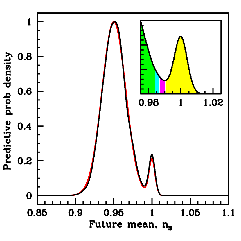
Figure 1: Predictive data distribution for the Planck satellite nominal mission, conditional on current (WMAP3+ext) knowledge. We are plotting the probability distribution (normalized to the peak) of the future measurement of the spectral tilt. The bump at $n_{S}=1$ corresponds to the probability associated with the HZ model. The black curve is obtained numerically from MCMC chains (Eq. (15)) while the red is for the Gaussian approximation, Eq. (12). In the inset, the shaded areas delimit regions where the Bayes factor from Planck deliver strong evidence in favour of $n_{S}\neq 1$ (green, $\ln\mathcal{B}_{01}<-5.0$, this region extending to all smaller $n_{S}$ values), moderate evidence for $n_{S}\neq 1$ (cyan, $-5.0\leq\ln\mathcal{B}_{01}\leq-2.5$), positive evidence for $n_{S}\neq 1$ (magenta, $-2.5\leq\ln\mathcal{B}_{01}\leq 0.0$) or favour $n_{S}=1$ (yellow, $\ln\mathcal{B}_{01}>0$). The corresponding probability values are reported in Table 1.

4.3 Dependence on the choice of prior

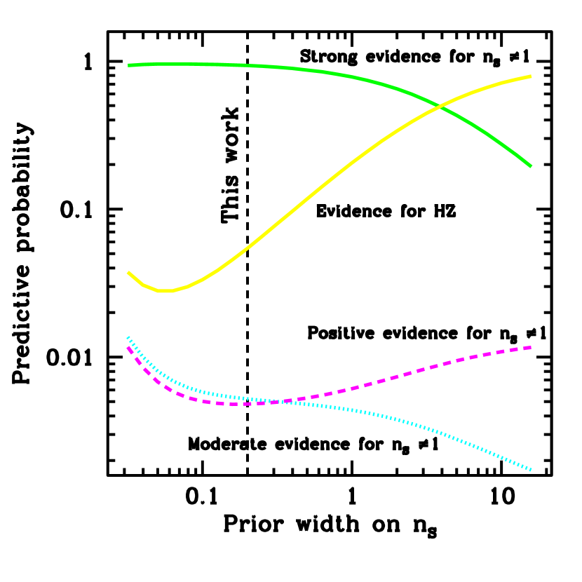
Figure 2: PPOD dependence on the prior width for $n_{S}$. We plot the PPOD result computed from the Gaussian approximation of Eq. (12) as a function of the width of the prior on $n_{S}$ for the model with $n_{S}\neq 1$. In order to change the conclusion of this work, namely that Planck has a large probability of conclusively measuring $n_{S}\neq 1$, one would have to adopt a prior larger than about 3.5 (crossing of the green and yellow lines). In this work, the prior width has been set to 0.2 (dotted, vertical line).

The prior assignment is an irreducible feature of Bayesian model selection, as it is clear from its presence in the denominator of Eq. (6). In fact, the prior width controls the strength of the Occam’s razor effect on the extended model, and thus a larger prior favours the simpler model.

We can assess the impact of a change of prior on our PPOD results by plotting them as a function of the chosen prior width. In Figure 2 we show how the probabilities for Planck to obtain different levels of evidence for or against $n_{s}\neq 1$ change with a change in the choice of the prior width $\Delta n_{S}$. It is apparent that our result holds true for a wide range of prior values: even if the prior is widened to $\Delta n_{S}=1$, the probability of a strong ($\ln\mathcal{B}_{01}<-5$, green line) result in favour of $n_{s}\neq 1$ is still about $80\%$. The prior width has to be enlarged to $\Delta n_{S}\,\raise 1.72218pt\hbox{$>$}\kern-6.99997pt\lower 2.6694pt\hbox{$\sim$}\,3.5$ for the simpler model to have more than 50% probability of being favoured (yellow line, depicting the probability of obtaining $\ln\mathcal{B}_{01}>0$).

5 Conclusions

We have presented a new statistical technique (PPOD) to produce forecasts for the probability distribution of the Bayes factor from future experiments. The use of PPOD can complement the Fisher matrix forecasts in that it allows to assess the capabilities of a future experiment to obtain a high–odds model selection result. Being conditional on present knowledge, our PPOD technique does not assume a fiducial model, but takes into account the current uncertainty in the values of the underlying model parameters.

We emphasize that the PPOD forecast, being conditional on the present posterior, is reliable provided there will be no major systematic shift in the parameter determination with respect to present–day data. In other words, the PPOD only takes into account the statistical properties of our knowledge, a point hardly worth highlighting (if we knew the outcome of a future measurement, it would be pointless to carry it out).

We have applied this method to a central parameter of the concordance model. We have found that the Planck satellite has over $90\%$ probability of obtaining a strong ($\ln\mathcal{B}_{01}<-5$) model selection result favouring $n_{S}\neq 1$ (for a prior width $\Delta n_{S}=0.2$), thus improving on current, moderate odds (of about $17:1$ or $\ln B_{01}=-2.86$). The probability that Planck will find evidence in favour of $n_{S}=1$ is by contrast only about $6\%$. These results are qualitatively unchanged for a wide range of prior values, encompassing most reasonable prior choices.

Acknowledgments I am grateful to Bruce Bassett and Tom Loredo for useful comments. I thank Martin Kunz, Andrew Liddle and Pia Mukherjee for helpful suggestions and comments on an early draft. This research is supported by the Royal Astronomical Society through the Sir Norman Lockyer Fellowship and by St Anne’s College, Oxford. The use of the Glamdring cluster of Oxford University is acknowledged. I acknowledge the use of the package cosmomc, available from cosmologist.info, and the use of the Legacy Archive for Microwave Background Data Analysis (LAMBDA). Support for LAMBDA is provided by the NASA Office of Space Science.

References

- Bassett (2005) Bassett B. A., 2005, Phys. Rev., D71, 083517
- Bassett et al. (2004) Bassett B. A., Corasaniti P. S., Kunz M., 2004, Astrophys. J., 617, L1
- Bassett et al. (2005) Bassett B. A., Parkinson D., Nichol R. C., 2005, Astrophys. J., 626, L1-L4
- Beltran et al. (2005) Beltran M., Garcia-Bellido J., Lesgourgues J., Liddle A. R., Slosar A., 2005, Phys. Rev., D71, 063532
- Bevis et al. (2007) Bevis N., Hindmarsh M., Kunz M., Urrestilla J., 2007, astro-ph/0702223
- Drell et al. (2000) Drell P. S., Loredo T. J., Wasserman I., 2000, Astrophys. J., 530, 593
- Efstathiou & Bond (1999) Efstathiou G., Bond J. R., 1999, Mon. Not. Roy. Astron. Soc., 304, 75
- Ford (2004) Ford E. B., 2004, preprint: astro-ph/0412703
- Freedman et al. (2001) Freedman W. L., et al., 2001, Astrophys. J., 553, 47
- Hinshaw et al. (2006) Hinshaw G., et al., 2006, astro-ph/0603451
- Hobson & McLachlan (2003) Hobson M. P., McLachlan C., 2003, Mon. Not. Roy. Astron. Soc., 338, 765
- Jaynes (2003) Jaynes E., 2003, Probability Theory. The logic of science. Cambridge University Press, Cambridge, U.K.
- Jeffreys (1961) Jeffreys H., 1961, Theory of probability, 3rd edn. OUP
- Kass & Raftery (1995) Kass R., Raftery A., 1995, J. Amer. Stat. Assoc., 90, 773
- Knox (1995) Knox L., 1995, Phys. Rev., D52, 4307
- Kosowsky et al. (1996) Kosowsky A., Kamionkowski M., Jungman G., Spergel D. N., 1996, Nucl. Phys. Proc. Suppl., 51B, 49
- Kosowsky et al. (2002) Kosowsky A., Milosavljevic M., Jimenez R., 2002, Phys. Rev., D66, 063007
- Kunz et al. (2006) Kunz M., Trotta R., Parkinson D., 2006, Phys. Rev., D74, 023503
- Kuo et al. (2004) Kuo C.-l., et al., 2004, Astrophys. J., 600, 32
- Lazarides et al. (2004) Lazarides G., de Austri R. R., Trotta R., 2004, Phys. Rev., D70, 123527
- Leach & Liddle (2003) Leach S. M., Liddle A. R., 2003, Phys. Rev., D68, 123508
- Lewis & Bridle (2002) Lewis A., Bridle S., 2002, Phys. Rev., D66, 103511
- Liddle (2007) Liddle A. R., 2007, Mon. Not. Roy. Astron. Soc. Lett. 377, L74-L78
- Liddle et al, (2007) Liddle A. R. et al, 2007, astro-ph/0703285
- Loredo (2003) Loredo T. J., 2003, in AIP Conf. Proc. ed., Proceedings of 23rd Annual Conference on Bayesian Methods and Maximum Entropy in Science and Engineering, Jackson Hole, Wyoming, 3-8 Aug 2003 ‘Bayesian adaptive exploration’. pp 330–346
- Loredo & Lamb (2002) Loredo T. J., Lamb D. Q., 2002, Phys. Rev., D65, 063002
- MacKay (2003) MacKay D., 2003, Information theory, inference, and learning algorithms. Cambridge University Press, Cambridge, U.K.
- Magueijo & Sorkin (2007) Magueijo J., Sorkin R. D., 2007, Mon. Not. Roy. Astron. Soc. Lett, 377, L39-L43
- Marshall et al. (2006) Marshall P., Rajguru N., Slosar A., 2006, Phys. Rev., D73, 067302
- Mukherjee et al. (2006) Mukherjee P., Parkinson D., Corasaniti P. S., Liddle A. R., Kunz M., 2006, Mon. Not. Roy. Astron. Soc., 369, 1725
- Mukherjee et al. (2006) Mukherjee P., Parkinson D., Liddle A. R., 2006, Astrophys. J., 638, L51
- Page et al. (2006) Page L., et al., 2006, astro-ph/0603450
- Pahud et al. (2006) Pahud C., Liddle A. R., Mukherjee P., Parkinson D., 2006, Phys. Rev., D73, 123524
- Pahud et al. (2007) Pahud C., Liddle A. R., Mukherjee P., Parkinson D., 2007, astro-ph/0701481
- Parkinson et al. (2007) Parkinson D., et al., 2007, astro-ph/0702040
- Parkinson et al. (2006) Parkinson D., Mukherjee P., Liddle A. R., 2006, Phys. Rev., D73, 123523
- Readhead et al. (2004) Readhead A. C. S., et al., 2004, Astrophys. J., 609, 498
- Riess et al. (2004) Riess A. G., et al., 2004, Astrophys. J., 607, 665
- Rocha et al. (2004) Rocha G., Trotta R., Martins C., Melchiorri A., Avelino P., Bean R., Viana P., 2004, Mon. Not. Roy. Astron. Soc., 352, 20
- Saini et al. (2004) Saini T. D., Weller J., Bridle S. L., 2004, Mon. Not. Roy. Astron. Soc., 348, 603
- Skilling (2004) Skilling J., 2004, Nested sampling for general Bayesian computation, available from: http://www.inference.phy.cam.ac.uk/bayesys
- Slosar et al. (2003) Slosar A., et al., 2003, Mon. Not. Roy. Astron. Soc., 341, L29
- Tegmark et al. (2004) Tegmark M., et al., 2004, Astrophys. J., 606, 702
- Trotta (2005) Trotta R., 2005, Available as v1 from astro-ph/0504022-v1
- Trotta (2007a) Trotta R., 2007a, Mon, Not. R. Astron. Soc., 375, L26, astro-ph/0608116
- Trotta (2007b) Trotta R., 2007b, New Astron. Rev., 51, 316, astro-ph/0607496.
- Trotta (2007c) Trotta R., 2007c, Mon. Not. Roy. Astron. Soc. in press, astro-ph/0504022