The PN.S Elliptical Galaxy Survey: Data Reduction, Planetary Nebula Catalog, and Basic Dynamics for NGC 3379

Abstract

We present results from Planetary Nebula Spectrograph (PN.S) observations of the elliptical galaxy NGC 3379 and a description of the data reduction pipeline. We detected 214 planetary nebulae of which 191 are ascribed to NGC 3379, and 23 to the companion galaxy NGC 3384. Comparison with data from the literature show that the PN.S velocities have an internal error of $\lesssim 20$ km s^-1and a possible offset of similar magnitude. We present the results of kinematic modelling and show that the PN kinematics are consistent with absorption-line data in the region where they overlap. The resulting combined kinematic data set, running from the center of NGC 3379 out to more than seven effective radii ($R_{\rm eff}$), reveals a mean rotation velocity that is small compared to the random velocities, and a dispersion profile that declines rapidly with radius. From a series of Jeans dynamical models we find the $B$-band mass-to-light ratio inside five $R_{\rm eff}$ to be 8 to 12 in solar units, and the dark matter fraction inside this radius to be less than 40%. We compare these and other results of dynamical analysis with those of dark-matter-dominated merger simulations, finding that significant discrepancies remain, reiterating the question of whether NGC 3379 has the kind of dark matter halo that the current $\Lambda$CDM paradigm requires.

1. Introduction

The confirmation in the 1970s that dark matter dominates the mass of the Universe came about from dynamical studies of spiral galaxies (Freeman, 1970; Ostriker & Peebles, 1973; Rubin et al., 1978; van Albada & Sancisi, 1986). In these systems, the HI gas disks offer the ideal diagnostic, since their extended nature allows one to probe very large radii where dark matter begins to dominate, and their cold disk-like structure ensures that the material is following approximately circular orbits, removing a major ambiguity in the study of its dynamics.

A similar study of elliptical galaxies would be invaluable, as it would address such basic questions as whether the dark matter halos around these systems are similar to those around spirals, suggesting that the difference in observed morphology is just a matter of frippery, or that there are more fundamental differences between them. Unfortunately the paucity of neutral hydrogen gas in ellipticals makes such a study observationally difficult.

Various dynamical tracers have been utilised to circumvent this problem. For example, some ellipticals do contain significant amounts of gas, either in the form of rings of cold material (e.g. Bertola et al., 1993; Franx et al., 1994; Oosterloo et al., 2002), or as a fuzzy halo of hot material (e.g. Buote & Canizares, 1994). Neither is entirely satisfactory as a tracer, though, as these systems are not usually what might be thought of as “normal” ellipticals: something peculiar must have happened to the galaxy to bestow it with a gas ring, while X-ray emitting halos tend to only be measured in the brightest systems, and are often confused with a surrounding intra-cluster medium. Other dynamical tracers such as globular clusters have also been employed (e.g. Pierce et al., 2006), but the relatively modest numbers that have been observed to date in normal ellipticals stand no chance of solving for the full distribution function of these objects, in order to allow for all the possibilities in their orbital distribution. Integrated-light absorption line spectroscopy has shown that the circular velocity profiles of ellipticals are typically flat to 2$R_{\rm eff}$, and that in a fraction of the galaxies analysed the dark matter contributes $\sim 10-40\%$ of the mass within $R_{\rm eff}$  when the stellar distribution has maximum mass, while in others no evidence for any non-stellar matter is seen to 2$R_{\rm eff}$ (e.g. Kronawitter et al., 2000; Gerhard et al., 2001; Magorrian & Ballantyne, 2001; Thomas, 2006).

For many years now, planetary nebulae (PNe) have been used to extend stellar kinematic studies to larger radii, where the sought-after dark matter is expected to dominate the potential, and where the stellar orbital timescale becomes long enough that some record of a galaxy’s formation is likely to have been preserved. Their bright 5007Å [O iii] line is relatively easy to detect and provides a line-of-sight velocity. Such measurements allow the velocities of stars to be measured out to arbitrarily large radii in elliptical galaxies; in fact, PNe become easier to detect at larger radii where the background light from the galaxy is fainter, so they neatly complement absorption-line studies at smaller radii.

A number of attempts have been made to exploit this possibility, generally by using narrow-band imaging to identify PNe, and follow-up spectroscopy to obtain their velocities. This approach has been fruitful (e.g. Ciardullo et al., 1993; Arnaboldi et al., 1998), but the two-step process, requiring precise astrometry, has tended to produce low yields.

Tremblay et al. (1995) and Sluis & Williams (2006) have shown that one can detect PNe and measure their velocities using a Fabry–Perot interferometer, now reaching sizable samples. Meanwhile, Douglas & Taylor (1999) developed the technique, coined “counter-dispersed imaging” , in which images are obtained using a slitless spectrograph with the dispersive element rotated by 180 degrees between exposures. The emission lines from PNe appear as unresolved dots in each of the dispersed images, shifted in opposite directions by an amount proportional to their velocities. By matching up the pairs of dots and measuring the distance between them, one can simultaneously identify PNe and measure their velocities. This technique was successfully implemented by Douglas et al. (2000) to study the kinematics of PNe in M94. Méndez et al. (2001) and Teodorescu et al. (2005) subsequently used a dispersed-undispersed imaging technique to measure the velocities of 531 PNe in NGC 4697 and 197 PNe in NGC 1344. The Planetary Nebula Spectrograph again utilizes counter-dispersed imaging but now two spectrographic cameras, fed by a beam-splitter arrangement at the grating module, are simultaneously in operation. Matched image pairs, from the same collimated beam and via the same filter at the same temperature, are therefore guaranteed. A more detailed description of the instrument is given in Douglas et al. (2002), and Figure 11 of that paper shows an example of the images obtained.

The PN.S has proved an effective tool for studying PN kinematics in a variety of environments. For example, we have completed a kinematic survey of M31, the resulting velocities of 2800 PNe allowing us to model the dynamics of this system in unprecedented detail (Merrett et al., 2006). However, the primary purpose of the instrument is to study the dynamics of a sample of ordinary early-type galaxies. We commenced this core project during commissioning of the instrument in 2001, with the intention of carrying out an extensive and definitive study of the large-scale dynamics of elliptical galaxies with a range of internal properties and in a variety of environments. Our initial finding was unexpected. The velocity dispersions of the first three galaxies we had observed did not remain roughly constant with radius as the simplest dark halo models would predict; instead they went into a Keplerian decline that was consistent with these systems having no dark halos at all (Romanowsky et al., 2003, hereafter R+03). Although such behaviour had been seen before (Ciardullo et al., 1993; Méndez et al., 2001), our findings provided the first strong indication that it might be a generic property of some types of ellipticals.

Subsequently, attention was drawn by Dekel et al. (2005) [hereafter D+05] to the well-documented degeneracy in the study of velocity dispersion profiles, that one cannot unambiguously disentangle the effects of mass distribution and orbital structure (Binney & Mamon, 1982): a declining profile could indicate a radial bias in the distribution of orbits instead of the lack of a dark halo. (R+03) had dealt with this possibility in some detail, and full orbit modeling for the case of NGC 3379 showed that, although some dark matter could be happily accommodated by this ambiguity, the results were still inconsistent with the standard cosmological predictions. However, further analysis has indicated that $\Lambda$CDM (cold dark matter) halos are not entirely ruled out by the published data (Mamon & Łokas, 2005, hereafter MŁ05), while studies of the kinematics of globular clusters around NGC 3379 seem to favor a more massive halo (Pierce et al., 2006; Bergond et al., 2006). D+05, citing the work of Marigo et al. (2004), also introduced the worrying possibility that the detected, brighter, PNe might not be drawn from the stellar population as a whole, instead being skewed toward a non-representative younger sample of stars. However, the observed universality of the bright end of the PN luminosity function (Ciardullo et al., 1989b, 2002) and the lack of variation in kinematics with PN luminosity down to very faint limits in the disk of M31 would tend to argue that this is not the case (Merrett et al., 2006).

In R+03 space did not allow us to present the full data reduction procedure, and so convince the reader that the novel PN.S instrument could be relied on to produce consistent and credible results, and that the inferred peculiar dynamics could not be attributed to some strange systematic problem with the unusual data analysis required. This issue is particularly pertinent because at the time the paper was written we were still investigating the optimum procedure for processing PN.S data. The full preliminary catalog of PN positions and velocities was also not published in the Science paper, making it difficult for others to reanalyze the dynamics using all the relevant information.

It is the purpose of this paper to address these issues. We will describe the now-finalized pipeline for analyzing PN.S data in some detail in §2. We present the complete set of PN.S observational data for NGC 3379 in §3. Since a number of smaller PN data sets already exist for this galaxy, we have been able to calibrate the reliability of the PN.S pipeline, as set out in §4. As a result of the improved data reduction and a larger amount of integration time, the catalog for NGC 3379 presented here contains approximately double the number of PNe that went into the analysis of R+03. We have therefore been able to make a more detailed analysis of issues such as completeness and contamination by other sources in §5, as well as comparing the properties of the PNe to the more general stellar population in §6, to address the contentious question of how well PNe trace the bulk stellar component. Although this paper is not intended to provide a definitive study of the dynamics of NGC 3379, §7 presents a descriptive overview of its observed kinematics, while §8 provides a more quantitative Jeans analysis of the galaxy’s dynamics to re-examine the contentious questions regarding the nature of its dark halo, if any. §9 takes another look at the question of whether or not the kinematic data from NGC 3379 is consistent with it having a standard $\Lambda$CDM dark halo as advocated by D+05, and we summarize the work in §10.

2. The Reduction Pipeline

As described in detail in Douglas et al. (2002), the PN.S is mounted as a visitor instrument on the William Herschel 4.2m telescope, operated by the Isaac Newton Group on the Island of La Palma. It effectively comprises a pair of slitless spectrographs, dispersed in opposite directions, with a common field of view of approximately $11^{\prime}\times 10^{\prime}$. The dispersion is 1.29 pxl/Å when used with the standard CCD (see below) and the plate scale is 3.67 pxl/^′′(somewhat less in the dispersed direction). A narrow-band filter restricts the spectral range, so stars are dispersed into short “star trails” while an object such as a PN, with a single emission line within the filter passband, appears as an unresolved dot in each of the two arms of the spectrograph, which we have arbitrarily labeled “left” and “right”.

In addition to conventional bias frames, sky flats, dome flats and flux calibrations with the aid of standard stars, we also obtain images through a mask that we can insert into the beam. The mask contains an array of 178 0.9^′′ holes at calibrated locations, and is illuminated with either a tungsten continuum lamp to determine the filter bandpass or a Cu-Ne-Ar lamp to determine the wavelength solution and spatial distortions.

Data reduction is via a dedicated pipeline written in the iraf script language, with some additional routines written in fortran. Because of its non-standard nature and its importance to the interpretation of the derived PN kinematics, we now describe the pipeline processes in some detail.

2.1. Initial Processing

The PN.S uses as its detectors a pair of 2k$\times$4k 13.5$\mu m$ pixel EEV CCDs maintained by the Isaac Newton Group itself, simplifying the integration of the PN.S within the Observatory’s data acquisition system. The first step in data reduction is to trim the data frames to the $2154\times 2500$ pixels that are illuminated by the spectrograph. There is little structure in the bias levels of these CCDs, so debiassing is achieved by subtracting a polynomial surface fitted to the under- and over-scan regions of the CCD. Bad pixels on the CCDs are identified using unsharp masking of sky or dome flats. The flats are combined to enhance their signal-to-noise ratio and remove cosmic rays, and are then compared to a median-smoothed version of the averaged flat. Any pixels that are deviant by more than 9$\sigma$ are flagged as bad. In addition, we maintain a library of known defects in these chips. From these bad pixel lists, we construct a binary mask of defects, and interpolate over bad columns using the iraf task fixpix.

2.2. Cosmic Ray Removal

We have experimented with different methods for the removal of cosmic rays. In the M31 survey (Merrett et al., 2006), the l.a.cosmic algorithm (van Dokkum, 2001) was used successfully. However, for longer integration times several iterations were required for even an imperfect correction which left residuals that could be confused with objects. We therefore devised a simpler routine, crcleankk, which examines each pixel’s neighbors to see if the gradient to these adjacent pixels is consistent with the local brightness and the seeing under which the data were obtained. Any pixels where this gradient is found to be too high are flagged as cosmic rays and removed.

2.3. Flatfielding

Sensitivity variations from pixel to pixel are calibrated using twilight sky flats. A customized script, ppcorrect, first creates a series of normalised flat field images by dividing each sky exposure by a median-filtered version of itself. These flats are then combined with a rejection threshold to eliminate residual cosmic rays, and weighted to maintain Poisson error characteristics. The resulting master flats for the left and right arms of the spectrograph are then applied to all the science and calibration frames to remove pixel-to-pixel variations.

The overall vignetting of the spectrograph is a little harder to quantify. The PN.S uses a slow shutter that takes $\sim 15$ seconds to open or close, so the effective exposure time varies somewhat across the field. This effect is completely negligible for science exposures, with typical integration times of a half an hour, but does affect the illumination of short twilight sky exposures significantly, so these data cannot be used to calibrate the vignetting function of the telescope. Instead, we measure the over-all illumination pattern using dome flats, for which the slow shutter is not an issue as the exposure time is determined by switching the lamps on and off. One problem with such flats is that the illumination of the inside of the dome tends to contain gradients due to the placement of the illuminating lamps. We have overcome this issue by combining dome flats obtained with the instrument rotator at a number of position angles, thus averaging away any such gradients.

2.4. Wavelength Calibration and Image Rectification

We now reach the heart of the pipeline. What most complicates the analysis of these slitless spectroscopic data is that, at least in one dimension, position on the CCD does not map directly from a single location on the sky: the dispersive element means that this coordinate encodes a combination of position and wavelength. To disentangle these effects, we utilise the Cu-Ne-Ar arc lamps of the calibration unit of the WHT, close to the focal plane, obtaining the images of several lines for each of the 178 apertures in the calibration mask. The instrumental setup is as close as possible to that during PNe observations, and includes the same narrow-band filter. This limits the number of arc lines seen to $\sim 5$, which is however sufficient. An automated task, alignspots, locates and centroids the spots on the CCD, and feeds these data to a routine which fits a joint polynomial fit for position and wavelength. The fitting orders used have been standardized by experiment, and residuals can be inspected graphically, drawing attention to systematic errors. The solution represents a map from particular positions in the sky reference frame, $\{X,Y\}$, and wavelength, $\lambda$, to a position on the CCD, $\{x,y\}$:

$$\{x,y\}=f(X,Y,\lambda).$$ (1)

This mapping is, of course, not one-to-one, since different combinations of position and wavelength will fall in the same CCD pixel, but the essence of the counter-dispersed technique is that the two arms of the spectrograph provide two independent mappings to positions on the two CCDs, $\{x_{L},y_{L}\}$ and $\{x_{R},y_{R}\}$, both of which are calibrated as above. As long as any pairs of detected sources can be matched up unambiguously, the mappings that we have obtained from equation 1 can be uniquely inverted to transform

$$\{x_{L},y_{L},x_{R},y_{R}\}\rightarrow\{X,Y,\lambda\}.$$ (2)

This inversion is ultimately performed by a pipeline script called pnsvel, which also converts the wavelength of the emission-line source into a velocity, under the assumption that the line in question is the [O iii] one with a rest wavelength of 5006.8Å. These velocities are converted to heliocentric values using the iraf task rvcorrect. The mapping functions of equation 2 also allow us to rectify the spatial distortions introduced by the spectrograph, and transform the images to “true” sky coordinates, using the iraf commands geomap and geotrans. For any individual image, this transformation is not really necessary since we have all the information for recovering sky coordinates encoded in equation 2, but it is required for the next step of combining exposures taken at different times.

2.5. Image Combining

Once the individual images from the two arms are rectified, they can be aligned and added to produce the final left and right image pair. It is possible that there might also be some degree of rotation or change in image scale between exposures obtained over a series of nights, or even from different observing seasons; we have allowed for this possibility in our routine to combine images, but have found in practice that it does not occur at a significant level.

One challenge here is that we do not have any bright point sources that we can use to register the different images. Even the brightest PNe are barely detectable in individual frames, so cannot be used to determine the offsets. Instead, we utilise the star trails described earlier in this section to align images. The locations of stars are determined using a task called xstartrails, which cross-correlates the star trails in the images with simulated trails, to determine their centroids. Given the greater extent of the star trails in the spectral direction, we might expect the coordinates to be less well determined in this direction, but since the offsets are determined using many (typically 10-15) star trails, positional accuracy is not significantly limited by this effect (see §4).

One slight subtlety in this alignment process is that the sub-pixel shifting of images to a common reference frame requires an interpolation of the data. Some information is lost with each such interpolation, and the image rectification applied in §2.4 means that we have already made one such transformation. Rather than applying a further transformation, we instead go back to the original unrectified images, and apply a single transformation that encompasses both the geometric correction and the shift to a common reference frame.

In addition to finding relative offsets between images, xstartrails can also be used to determine an absolute astrometric reference frame for the data. It does so by reading in the positions of a number of suitable stars for the appropriate field from the USNO-B catalog (Monet et al., 2003) and applying the proper motion correction to the epoch of the observation. In a typical high-latitude field, there are 30 – 40 stars in this catalog at magnitudes $B<20$, which cause bright enough star trails to be easily detected. The approach to wavelength calibration that we have adopted means that the center of the star trail is mapped onto the CCD via equation 1 at a location corresponding to the star’s sky coordinates and a wavelength given by the central wavelength of the narrow-band filter. We can therefore use the observed centroid of the star trail to define the absolute astrometric frame, although the poorer definition of the star trail’s centroid in the dispersed direction means that we would once again expect the reference frame to be less well determined in this direction. Fitting the observed locations to those in the USNO-B catalog with a low-order polynomial plate solution (quadratic in the dispersed direction and linear in the undispersed direction) gives a satisfactory fit with typical residuals of 1 – 2 arcseconds. Since the solution uses 30 – 40 stars, the random error from the fit will be significantly smaller. As we will see in §4, absolute coordinates are tied down by this procedure to better than an arcsecond in both the dispersed and undispersed directions, which is entirely adequate for this survey.

In order to combine the individual data frames appropriately, xstartrails also evaluates the quality of each exposure to determine how much weight it should have in the final co-added image. Specifically, the task estimates the seeing full-width at half maximum, $\varsigma$, by taking a cut through the star trails in the undispersed direction, it determines the relative transparency, $\tau$, by comparing the brightnesses of star trails in different images (allowing for differences in exposure time, $t$), and it measures the sky background level, $B$, around the trails. To account for these quality indicators in creating a combined image, each frame is weighted by a factor

$$W={t\tau\over\varsigma^{2}B}.$$ (3)

With this scaling, images with the same quality but different exposure times will be weighted equally, since $B\propto t$, and the final combined images for each arm optimally combine data taken in variable conditions.

2.6. Photometry

Although not primarily designed as a photometric instrument, the PN.S does provide some information on the brightnesses of the objects that it detects. Since the PN luminosity function is broad, and we typically detect PNe over a range of several magnitudes, even quite crude photometric measures are useful in, for example, trying to see if their kinematics vary with luminosity. To determine the absolute zero-point of the photometry, we observe a number of flux standard stars throughout each observing run. Because of the slow shutter speed, we adopted a different observational set-up for standards: leaving the shutter open, we let the time between the clear and the read-out of the CCD determine the integration time. The CCDs are windowed for this procedure, so there is no significant contamination of the standard star from additional flux during read-out.

As with any other star, the light from the standard star is dispersed by the PN.S into a short filter-limited star trail. The counts in each such trail are integrated over a small number of pixels in the dispersed direction at a point in the center of the trail corresponding to the peak of the filter transmission. These values are then turned into a photon detection rate by subtracting background counts derived from pixels surrounding the trail, converting from ADUs to electrons as appropriate for the CCD, correcting for the airmass of the observation, and dividing by the exposure time to get a rate. This count rate can then be compared to the fluxes provided by Oke (1990) and Stone (1982) to find the photometric conversion factor. Since the optical paths to the two arms differ, this process is carried out separately for each arm of the spectrograph.

One minor complication in applying this calibration to detected emission-line sources is that the observed counts will depend on the wavelength at which the source is detected: the more a source is Doppler-shifted towards an edge of the filter’s narrow bandpass, the more light will be lost. Further, the bandpass of the filter changes somewhat depending on the angle of the light’s incidence; since the filter is in the collimated beam, the bandpass will vary with position in the field of view. We therefore, during daytime, obtain long-exposure continuum lamp images through the mask in order to map out these effects. This calibration procedure is a significant improvement over what is possible in traditional narrow-band surveys, where the same effects occur, but where detailed determination of the bandpass is more problematic. In practice, the profile of the filter and the narrow range of angles involved mean that the correction that we apply to source fluxes (once their positions and wavelengths have been determined) is never more than $\sim 15\%$.

The other complicating factor is that observations can be undertaken at a wide range of air masses, and under varying photometric conditions. Fortunately, it is fairly straightforward to account for this by comparing the measured counts in the star trails with the counts obtained during the best conditions. Once again this task is carried out automatically using xstartrails.

Once these flux calibrations have been applied to the detected emission-line objects, the derived values can be converted to the usual $V$-band equivalent magnitude. To do so, it is assumed that the flux, $F_{\rm 5007}$, originates from the [O iii] line at 5007Å, in which case the equivalent magnitude is given by

$$m_{5007}\equiv-2.5\log[F_{\rm 5007}({\rm erg}\,{\rm s}^{-1}\,{\rm cm}^{-2})]-13.74$$ (4)

(Jacoby, 1989).

2.7. Object Finding

Perhaps the single most important element in the pipeline is the detection of sources in the final images. A careful balance must be struck between being too optimistic and identifying noise spikes as objects, and being too pessimistic and throwing out valid sources from the ultimate catalog. An extra factor here is that a source must be detected in both arms of the spectrograph to return a velocity, so we need also to consider the optimum way to process the data to obtain coincident detections. We have therefore invested considerable effort into optimizing this process, looking at both visual inspection and semi-automated techniques. Our conclusion is that both approaches have their merits: the automated algorithms are better at assessing the significance of faint object “detections,” while the human approach is better at dealing with non-standard situations such as an object very close to a star trail. We have therefore opted to perform both types of analysis, each separately carried out by two researchers, resulting in a total of four independently-derived catalogs. Once the separate lists are produced in this independent manner, they can be compared to assess their efficiencies, and any discrepancies can be dealt with via an agreed dispute resolution process.

For the automated procedure, initial identification of sources is carried out using SExtractor (Bertin & Arnouts, 1996). To reduce the effects of large-scale diffuse light from the galaxy, the stacked image obtained from each arm is first median subtracted, using a $49\times 49$ pixel kernel to define the median around each pixel. The input parameters for SExtractor were tested on artificial images in order to find an optimal compromise between object finding and spurious detections. Groups of at least 5 contiguous pixels whose flux above the background is at least 0.7 times the rms of the background are classified as potential sources. The choice of criteria for separating point-like PNe from extended background sources is left to the individual researcher carrying out the search, as different sets of criteria seem to produce similar results, and we want to test how sensitive the results are to the specific criteria adopted. Spurious objects are eliminated by cross correlation of the catalogues produced for the left and right arm respectively. The researchers using the automated procedure then inspect the identified sources by eye to make sure that the algorithm has not been fooled by star trails or other spurious features.

The researchers who draw the short straws carry out the entire procedure by eye, laboriously going over every part of the images from the two arms of the spectrograph, blinking between them to look for pairs of point-like objects that appear at the appropriate locations to be the signature of a PN.

Once each catalog of potential emission-line objects has been compiled for the left and right arms of the instrument, they can then be matched up in an automated algorithm to convert their locations on the two CCDs into a position on the sky and a velocity, as in equation 2. The primary criterion for searching is that the detections in the two arms have to lie at the same coordinate in the undispersed direction to within two pixels (set to accommodate the maximum positional uncertainty in the faintest sources). In the dispersed direction, the coordinates must match up to within 200 pixels, since a separation greater than this would correspond to a wavelength outside the filter bandpass. In the small number of cases where the field is sufficiently crowded that more than one match between pairs is possible, we use the fluxes of the sources to resolve the ambiguity where possible. In the end, there are very few apparent detections which are not allocated to a unique matched pair. From the resulting four independent lists of objects, a “core catalog” is constructed where all four agree that a source had been detected. A “dispute catalog” contains the remaining sources that were not found in all four searches. These disputed objects are all inspected independently by the four catalogers. Those cases where all now agree that the source is real are combined with the core catalog to produce a “consensus catalog.” Objects that are significantly extended are placed in the “extended catalog” for later study, and for exclusion from the PN analysis. Finally, to produce the most uniform data set possible, a signal-to-noise ratio cut of five (in each arm) is applied to produce the “final catalog.”

3. Application to NGC 3379 Observations

As a first application of the data reduction pipeline, we have analyzed PN.S observations of NGC 3379. This galaxy provides a good initial test case for a number of reasons. As an E1 galaxy at a distance of 9.8 Mpc (Jensen et al., 2003), with an absolute magnitude of $M_{B}=-19.8$ and an effective radius of $R_{\rm eff}$=47^′′ (see §8.2) corresponding to 2.2 kpc, it is fairly typical of the systems in our survey of ordinary elliptical galaxies. Also, since NGC 3379 was one of the objects in R+03, we can check that the initial results are confirmed, and can see how much better we can do with the fully-developed pipeline than was possible with our earlier procedure. There also exists a number of smaller PN data sets from NGC 3379, which we can compare to our results as a test of the reliability of the PN.S and its pipeline-processing. As Table 1 shows, we have obtained some 19 hours of integration on this object under a variety of seeing conditions over multiple observing seasons, so we can also test our ability to combine such heterogeneous data into an effective stacked image. Using the scaling relationship that point-source detectability goes as the inverse square of the seeing, these observations are the equivalent of 7 hours observing in nominal one arcsecond seeing, which is typical of the depth to which our elliptical galaxy survey is being made.

Table 1Log of NGC 3379 Observations

Date	Integration	Seeing
	(hours)	(FWHM)
2002 March 7	2.0	1.9′′
2002 March 8	4.8	2.5′′
2002 March 9	1.5	1.4′′
2002 March 10	2.5	1.4′′
2002 March 14	2.6	2.5′′
2003 March 1	2.0	1.1′′
2003 March 4	1.6	1.7′′
2003 March 6	0.3	1.2′′
2003 March 7	1.5	1.2′′

NGC 3379 has a systemic velocity of 910 km s^-1, so the observations were made using our “B” narrow-band filter, which has a default nominal central wavelength of $5033.9$ Å and FWHM of 31 Å. This central wavelength was shifted to $5026.74$ Å by tilting the filter by 6 degrees, as described in Douglas et al. (2002). One side effect of tilting the filter is that the bandpass varies more significantly with position in the field of view. To compensate for this effect, the pointing was offset by 2^′ from the center of the field, but the relatively small size of the galaxy and the 10^′ field of PN.S mean that the observations still reach easily to beyond 7 $R_{\rm eff}$. The instrument position angle was set to $90^{\circ}$, such that the grating dispersed in the East-West direction.

Table 2Flux Calibration

Star Name	$C_{L}$	$C_{R}$	$E_{L+R}$
(1)	(2)	(2)	(3)
Feige 67	$2.22\times 10^{-16}$	$2.04\times 10^{-16}$	0.27
Feige 67	$2.26\times 10^{-16}$	$2.07\times 10^{-16}$	0.26
Feige 98	$2.07\times 10^{-16}$	$1.92\times 10^{-16}$	0.29
Feige 98	$2.10\times 10^{-16}$	$1.91\times 10^{-16}$	0.28
Median	$2.16\times 10^{-16}$	$1.98\times 10^{-16}$	0.28

NOTES – (1): Flux standard’s name. (2): Conversion factors in units of erg s^-1 cm^-2 Å^-1 / $e^{-}$ s^-1 Å^-1 for the left and right arms. The median value is shown at the bottom of the table. (3): Total efficiency of the instrument, $E_{L+R}=\frac{\epsilon}{(C_{L}+C_{R})S}$, where $\epsilon=3.95\times 10^{-12}\,{\rm erg}$ is the energy per photon at the observed wavelength of 5026.74 Å, and $S$ is the total collecting area of the telescope.

We also observed a number of flux standard stars and carried out the photometric calibration as set out in §2.6. The results are presented in Table 2, which also gives a sense of the level of uncertainty in the photometric calibration of PN.S data. The table additionally shows the derived total efficiency of telescope-plus-instrument, which lies close to the design specification of 30%.

Table 3Catalog of PNe in NGC 3379

ID	RA	Dec	wavelength	$v_{\rm helio}$	$m_{\rm 5007}$	SW06	CJD93
PNS-EPN-	J2000	J2000	Å	km s-1
NGC3379 1	10:47:31.22	12:39:20.3	5023.7	1005	27.04	–	–
NGC3379 2	10:47:32.23	12:32:09.9	5022.1	909	26.55	–	–
NGC3379 3	10:47:33.61	12:34:08.7	5021.8	892	27.67	–	–
NGC3379 4	10:47:34.43	12:35:54.1	5022.9	958	26.89	–	–
NGC3379 5	10:47:34.83	12:34:40.4	5024.3	1038	27.83	–	–
NGC3379 6	10:47:35.27	12:36:48.1	5021.5	874	27.15	–	–
NGC3379 7	10:47:35.96	12:33:51.1	5024.0	1024	26.95	–	–
NGC3379 8	10:47:36.35	12:33:54.0	5024.0	1022	26.51	–	77
NGC3379 9	10:47:36.44	12:33:05.8	5022.1	909	27.10	–	–
NGC3379 10	10:47:36.59	12:33:50.3	5024.4	1043	24.99	–	–
NGC3379 11	10:47:37.97	12:35:09.1	5021.8	890	27.99	–	–
NGC3379 12	10:47:38.06	12:34:58.1	5023.1	967	26.14	–	54
$\vdots$	$\vdots$	$\vdots$	$\vdots$	$\vdots$	$\vdots$	$\vdots$	$\vdots$
NGC3379 212	10:48:09.93	12:37:33.4	5020.7	824	8.63	–	–
NGC3379 213	10:48:10.08	12:35:49.8	5023.0	961	27.12	–	–
NGC3379 214	10:48:10.58	12:37:23.4	5021.4	868	26.39	–	–

NOTES - The PN.S data follow the usual definitions, and the ID is chosen to be compatible with proposed IAU standards (EPN standing for “Extragalactic Planetary Nebula”). The absence of a magnitude entry indicates that a reliable value could not be ascertained. Daggers indicate PNe which were allocated to NGC 3384 (see § 5.2). Columns SW06 and CJD93 show matching PNe in the catalogs of Sluis & Williams (2006) and Ciardullo et al. (1993) respectively. As is clearly indicated, two of the matches with Sluis & Williams (2006) are with PNe from their table 6 (NGC3384 catalogue). Objects were considered matched with a PN in our catalog if the positions agreed within 3.0^′′ and their velocities within 100 km s^-1 without adjustment for systematic offsets in either case. The full catalogue is available in the associated electronic material.

The NGC 3379 observations were pipeline-processed as described in §2, resulting in a consensus catalog of 214 objects, which have an overwhelming likelihood of being PNe. The dispute resolution procedure also produced a catalogue of 17 uncertain PNe. Of these, four had uncertain velocities because the pairs of objects in the two arms of the spectrograph could not be matched up unambiguously. Although such objects cannot be used in the kinematic studies, they are nonetheless firm detections, so must be included in other analyses such as the number count distribution. The final signal-to-noise ratio cut did not exclude any of the consensus detections, so the final product, the catalog of PNe, contains 214 PNe as presented in Table 3.

4. Comparison with Existing Data

One of the reasons for basing this initial application on the observations of NGC 3379 was that several smaller PN kinematic data sets already exist for this galaxy, so we can obtain an independent measure of the reliability of the data set. In addition to our own preliminary analysis of PN.S data, there are catalogs in the literature from Ciardullo et al. (1989a), Ciardullo et al. (1993) and Sluis & Williams (2006), which we now consider in turn.

4.1. Comparison with Romanowsky et al. (2003)

A simple internal check on the robustness of results derived from PN.S data is provided by a comparison of the current analysis with the ad hoc preliminary analysis that we performed on the same data in R+03. That preliminary analysis picked out 109 PNe in a first pass through the 2002 data, and the PN.S catalog matches 106 of these objects. The more detailed analysis in this paper has flagged the remaining three objects as extended, thus excluding them from the catalog. The new pipeline produces velocities with a positive offset of 34 km s^-1 from the earlier analysis, probably because the wavelength calibration can now be performed more accurately. The joint scatter for the 106 mutual objects is 22 km s^-1. Neither of these velocities is large enough to be relevant to the scientific results from the instrument.

4.2. Comparison with Ciardullo et al. (1989,1993)

Ciardullo et al. (1989a) measured positions and magnitudes for 93 PNe in NGC 3379 using the traditional on-band/off-band imaging technique, and then Ciardullo et al. (1993) followed this work up with velocity measurements of 29 of the PNe using multi-fiber spectroscopy. Comparing PN.S coordinates to these published values, we can with reasonable confidence match up 76 of the 93 sources on the basis of position (with a 3^′′search window), utilising radial velocity data where available to decide between ambiguous matches. If radial velocities are not available we take the best match on position and magnitude. Of the 17 PNe which were not matched by objects in our survey three were found to have been rejected as extended, five were embedded in star trails or lost in the galaxy’s diffuse light, and the remaining nine apparently lay below the magnitude limit of our data. Of the subset of 29 objects for which velocities were obtained by C+93, we are able to match 26 on the basis of position alone, using radial velocity data to eliminate just one ambigous match (PNS-109 with C+93-64). As expected, the differences in position are marginally larger in right ascension than they are in declination, as the stars from which our astrometric solution was derived are dispersed in this direction (see §2.5). However, the combined rms difference in position is only 1.6^′′, which is completely negligible in studying the dynamics of a system of this size.

Figure 1.— Comparison between the measured magnitudes (upper panel) and velocities (lower panel) for the PNe common to the Ciardullo et al. (1989a, 1993) and PN.S catalogs, as a function of apparent magnitude. Filled boxes show PNe identified in the PN.S catalog as members of NGC 3379, while open stars indicate members of NGC 3384.

We have also investigated differences in velocities and magnitudes. Figure 1 shows the correlation between magnitudes, and velocity differences, for common objects in the two catalogs. The velocities show a median offset of 28 km s^-1 and a scatter of 16 km s^-1, with no indication that the errors increase for fainter PNe. We also looked for systematic variations in the differences between the results with position in the field or with velocity itself, which might be expected if the wavelength calibration of the PN.S data contained undiagnosed systematic problems, but no such effects were apparent.

4.3. Comparison with Sluis & Williams (2006)

Sluis & Williams (2006) measured the positions, velocities and magnitudes for a sample of 54 PNe. Since these results were obtained using a Fabry–Perot interferometer, they are potentially subject to a different set of systematic effects, so provide yet another useful independent check on the reliability of our catalog. Of their objects, we recovered 39, with the remainder either masked in our data by star trails or at small radii where the PN.S has trouble recovering objects against the bright continuum of the galaxy (see §5.1). The difference in position for the matched pairs is even smaller than those for the Ciardullo et al. (1989a) set, with the rms combined difference being just 0.9^′′.

Figure 2.— Comparison between the measured magnitudes (upper panel) and velocities (lower panel) for the PNe common to the Sluis & Williams (2006) and PN.S catalogs, as a function of apparent magnitude. Symbols are as in Figure 1.

Figure 2 shows the differences between the magnitude correlation and the velocity differences, between common objects in the two catalogs. Once again, the velocities match up well, with a median offset between the two datasets of only 20 km s^-1, a combined scatter of 32 km s^-1, and no sign of any increase in error at faint magnitudes. There is again considerable scatter between magnitudes, though not much more than is evident between the external catalogues themselves (see Figure 3). Importantly, there are no trends which suggest that the measured velocities are correlated with magnitude in any way. Indeed a much more extensive analysis by Merrett et al. (2006) of the magnitudes of PNe in M31 returned by the PN.S compared to those from other surveys found no such trend, and we have carried out analogous tests which show that there is no indication for any systematic errors in velocity or magnitude with position in the PN.S field.

Figure 3.— Magnitude comparison between the catalogues of Sluis & Williams (2006) and Ciardullo et al. (1989a)

In summary, internal and external cross-checks have confirmed that there are no systematic effects that would compromise our measured velocity dispersions, and that the errors on individual PN velocities are at an entirely satisfactory level of $\sim 20\,{\rm km}\,{\rm s}^{-1}$.

5. Completeness and Contamination of the NGC 3379 PN Catalog

Before this catalog can be used for studying the dynamics of NGC 3379, it is important that we quantify what fraction of sources we may have missed, and that we remove any spurious sources that are unrelated to the target.

5.1. Completeness

We already have some sense of the likely completeness of the catalog by the fraction of previous identifications that we were able to recover in §4, which suggested a figure of about 80%, including a fairly constant fraction lost in star trails. However those comparisons are not adequate to determine the losses due to the diffuse brightness of the galaxy, which increases to smaller radius, making the fainter PNe progressively harder to identify. To quantify this effect, we have randomly placed simulated PNe in the data frames, and used the source searching algorithm of §2.7 to see what fraction are recovered. Fainter objects will obviously be harder to find, so we have populated the planetary nebula luminosity function to different faintness limits below $m^{*}$ (the magnitude of the brightest PNe given the known PNLF and distance, (Jacoby, 1989), here 25.48) to see how faint we can go. The simulations show that the detectability of even the brightest ($m^{*}$) PNe is essentially zero within a radius of $20^{\prime\prime}.$ For PNe with $m^{*}+1.0$ detectability rises sharply to a limiting value of 95% at $R\sim 100^{\prime\prime}$ radius, while for fainter PNe ($m^{*}+1.5$)detectability reaches a limit of 85% at the same radius. This nicely illustrates the complementarity between the study of stellar kinematics using PNe and those derived from conventional absorption-line spectroscopy: within one effective radius of $R_{\rm eff}$ = 47^′′ the diffuse background of the galaxy makes PNe very difficult to detect, but this same higher surface brightness makes absorption-line spectroscopy fairly straightforward.

We can, of course, correct for incompleteness when studying the PNe as a tracer population, but must be a little careful when doing so. If, for example, the PN kinematics varied significantly with their luminosity, then the observations at small radii, which preferentially detect the brightest PNe, would not be sampling the same dynamical population as those at large radii. Such a phenomenon has apparently been detected in NGC 4697 by Sambhus et al. (2006), but was not seen at all in M31 by Merrett et al. (2006). Nonetheless, care must be taken to test for such biases in any detailed dynamical study.

Perhaps of greater concern is the question of whether the probability of detection might depend on a PN’s velocity as well as its location, as such a bias would clearly compromise a dynamical study. The central wavelength of the narrow-band filter, as used in PN.S, varies only slightly over the field, the variation increasing with tilt. The bandwidth does not vary, to the limit of our measurements. When the filter has to be tilted the effects can be mitigated by appropriately changing the position of the target in the field of view. A typical situation is shown in Figure 4, demonstrating how kinematic bias can be avoided.

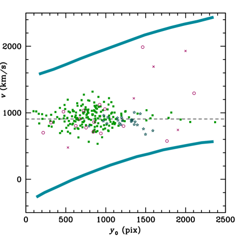
Figure 4.— Plot of velocity versus spatial coordinate in the direction in which the filter bandpass varies with position due to its tilt (here 6^∘). The points show the detected emission line objects in this observation: squares are PNe from NGC 3379; stars are PNe from NGC 3384; circles are extended sources; crosses are unresolved background sources. The thick lines mark the detection limits imposed by the filter FWHM bandpass.

One could imagine other kinematic biases arising from the few PN pairs which are discarded due to confusion, or from the impact of the central galaxy light on PN detections. However, we have performed simulations of these PN “losses” and verified that there is no significant velocity selection effect.

5.2. Contamination by NGC 3384 PNe

Having considered the sources that we may have missed, we now turn to excess sources that are not in NGC 3379. The SB0 galaxy NGC 3384 lies only 7^′ in projection away from NGC 3379, so their populations will appear to some extent superimposed. NGC 3384 has a systemic velocity of 704 km s^-1, some 200 km s^-1 lower than NGC 3379, but inconveniently NGC 3384 is rotating quite rapidly, and the side of NGC 3384 closest to NGC 3379 comprises the receding part of its disk, which shifts the velocity of any PNe to very close to NGC 3379’s velocity, so we cannot separate the two populations on the basis of their kinematics, as indeed another glance at Figure 4 immediately shows.

Instead, we adopt the simple approach of dividing the two on a probabilistic basis: we model the distributions of PNe in the two galaxies on the assumption that they follow the diffuse starlight, and assign each PN to whichever distribution makes the dominant contribution at its location. One slight subtlety is that because these galaxies lie at different distances and because their PN luminosity functions have somewhat different intrinsic specific frequencies (Ciardullo et al., 1989a), the cross-over between the two does not exactly coincide with the similar point in the raw photometry. However, these effects can be accounted for, and the resulting division between the two, which is shown in Figure 5, allocates 23 of the 214 PNe to NGC 3384. Although there is some residual uncertainty in this allocation, its impact is likely to be slight: we have found that the east-side and west-side kinematics of NGC 3379 remain symmetric even if we change the measurement radius from $200^{\prime\prime}$ to $240^{\prime\prime}$.

5.3. Contamination by non-PNe

The initial source identification of §2.7 has already flagged a number of sources as not being PNe because they are extended either spatially or spectrally. Visual inspection of an R-band image of the field identified many of these as star-forming background galaxies. At the distance of NGC 3379, even the largest PNe will be point sources, and the low expansion velocities of PNe mean that they should also appear unresolved spectrally, so we can immediately reject such objects. However, it is interesting to note that these sources are not uniformly spread spatially and in velocity, within the limits of the filter bandpass, as one would expect if they were simply background galaxies with emission lines that happen to fall within the filter. As Figure 4 shows, there is a definite concentration associated with the position and velocity of NGC 3379. Thus there may be a small population of extended emission-line nebulae associated with this galaxy, perhaps similar to the isolated, compact HII regions discovered in the low-gas density outskirts of other galaxies (Ferguson et al., 1998; Gerhard et al., 2002; Ryan-Weber et al., 2004). It would certainly be interesting to study them more closely both morphologically and spectroscopically with a more conventional instrument, but for the moment we simply exclude them because they are not part of the PN population that we are seeking to study dynamically.

In addition to these resolved objects, there are presumably some contaminants that are small and that only contain narrow emission lines, and so will not be flagged as extended. To try to identify such sources, we have used the “friendless” algorithm applied by Merrett et al. (2003), in which any object that lies more than $n$ standard deviations from the velocity distribution of its $N$ nearest neighbors is deemed not to be part of the general population due to its kinematic peculiarity. In this case, setting $n=3$ and $N=15$ identifies the 5 sources marked as crosses in Figure 4 as likely interlopers; as might be expected, they are spread fairly uniformly in position and velocity. These objects are therefore rejected from the default catalog, but we also test our results for robustness by seeing how much they change if we only reject the two friendless sources that we obtain by setting a more conservative $n=5$. This is dealt with in § 6.2.

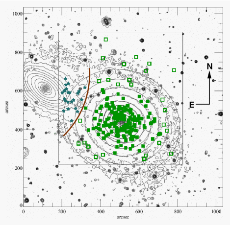
Figure 5.— $I$-band photometry from Cappellari et al. (2006), with the locations of detected PNe and the field of the PN.S observation marked. The heavy arc marks the division between the two galaxies for assigning membership to PNe, so squares are members of NGC 3379 while stars are members of NGC 3384. The filled symbols for NGC 3379 are used for objects that lie within the isophotal radius out to which the entire galaxy has been mapped.

6. Comparing Stellar and PN Properties

Having produced a clean sample of PNe from NGC 3379, we are now in a position to compare it to the properties of the unresolved stellar population. It is important to ascertain whether they are sampling the same underlying sources, as we can only exploit the potential synergy between absorption-line kinematics at small radii and PN.S results at large radii if they really form a single tracer population. We therefore now compare both photometric and kinematic properties of PNe to the results available for the diffuse stellar light to see how well they match up.

6.1. Spatial Distribution

The simplest comparison that we can make is between the number counts of PNe and the surface photometry of NGC 3379. To make a direct comparison, we must correct the number counts for incompleteness. As we have seen in §5.1, at small radii PNe are lost against the bright background of the galaxy, so we use the results of those simulations to determine the fraction that are missing and correct the PN counts accordingly. At large radii, the limited field of view of PN.S and the presence of NGC 3384 restrict the regions in which PNe can be found, so we must correct for this geometric factor by using the areas outlined in Figure 5 to determine the completeness of sampling.

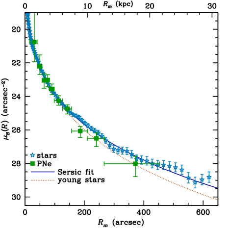
Figure 6.— Radial profiles of stars and PNe in NGC 3379. Stars show the stellar photometry, and squares the PN number counts, with an arbitrary vertical normalization. The PNe counts have been corrected for completeness (see § 5.1. Vertical error bars in this and subsequent figures show the 1-$\sigma$ uncertainties on the data (based on counting statistics and completeness correction uncertainties), while the horizontal bars show the radial range over which the PNe have been binned. The solid line is a Sersic (1968) profile fit to the stellar photometry, while the dotted line shows the profile for a hypothetical younger PN population (see text).

For the stellar photometry, we have used the wide-field $B$-band observations of Capaccioli et al. (1990), supplemented by the HST $V$-band photometry of Gebhardt et al. (2000) to fill in the photometry within the central 10^′′. The photometry has been matched up by assuming a constant color offset of $B-V=1.03$. Major axis profiles have been transformed into intermediate axis values, $R_{m}\equiv a\sqrt{1-\epsilon}$, using the ellipticities, $\epsilon$, from the same literature. At large and small radii the observational uncertainties in ellipticity become rather large, so we fix $\epsilon=0$ for $R_{m}<0.8^{\prime\prime}$, and $\epsilon=0.16$ for $R_{m}>40^{\prime\prime}$.

Figure 6 compares the PN number counts (to a limit of $m^{*}+1.5$) to the stellar photometry. Clearly, the two match up reasonably well, although there might be some indication that the PNe are more centrally concentrated. This possibility should be investigated, given the suggestion by D+05 that the PN kinematics of NGC 3379 could be driven by a younger population, which should also be more centrally concentrated. The figure therefore also shows a model for the spatial distribution that might be expected for such a young population, constructed by fitting a Sersic (1968) profile to the photometry (also shown in Figure 6), and multiplying it by an extra $R^{-0.3}$ power law, which approximately matches the difference between the young and total stellar profiles in the models of D+05. This model fits the PN number counts better than the raw stellar photometry, but no better than a third model (not shown) incorporating a mild metallicity gradient such as has been seen in other elliptical galaxies (Méndez et al., 2005).

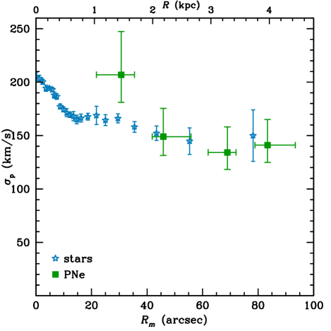
Figure 7.— Projected velocity dispersion profiles of stars (blue stars) and PNe (green squares) in the inner parts of NGC 3379. The stellar data are from Statler & Smecker-Hane (1999). Horizontal error bars show 68% of the radial range of the PNe.

6.2. Kinematics

Since the primary goal of this project is to map out the stellar kinematics of elliptical galaxies out to large radii, perhaps the most important comparison that we can make is between the kinematics derived from PNe and those from stellar absorption-line data. Fortunately, Statler & Smecker-Hane (1999) obtained deep long-slit absorption-line spectra of NGC 3379 at 8 different position angles. It is an indication of the difficulty in obtaining stellar kinematics out to large radii using conventional methods that even these data struggle to reach beyond 2 $R_{\rm eff}$. However, as we will see in §7, the kinematics of NGC 3379 are dominated by random motions, with little evidence for any azimuthal structure. We can therefore improve the signal-to-noise ratio without losing much dynamical information by averaging the rms velocity, $v_{\rm RMS}$, from the different position angles to form a single stellar velocity dispersion profile. Although the mean streaming velocity, $v$, is much smaller than the velocity dispersion, $\sigma$, at all radii along all position angles, we retain it in the rms velocity by defining $v_{\rm RMS}=\sqrt{v^{2}+\sigma^{2}}$. Figure 7 shows the resulting average dispersion profile, and compares it to the profile derived by binning the PNe in this range of radii in groups of $\sim 25$ and calculating the rms velocities in the resulting bins. To within the sizeable error bars, the kinematics of the PNe are indistinguishable from the stellar component.

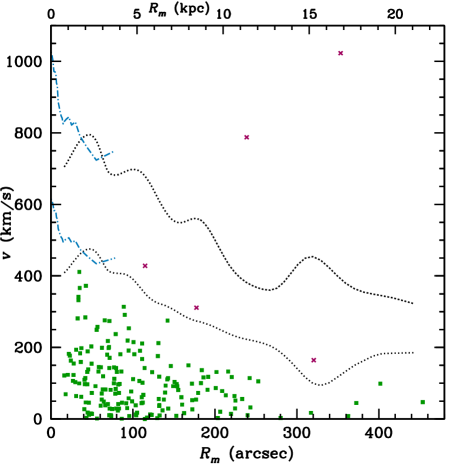
Figure 8.— Azimuthally-averaged velocity distribution of PNe in NGC 3379, plotted as a function of their projected radius. The dotted lines show the 3-$\sigma$ and 5-$\sigma$ envelopes of their velocity distribution (and the excluded unresolved point sources from §5.3 shown as crosses). The dash-dotted lines show the corresponding envelopes derived from the absorption-line stellar kinematics. A systemic velocity of 906 km s^-1 has been subtracted.

The marginally high first point for the PNe in Figure 7 is only $\sim 1.2\sigma$ away from the stellar data, so is not statistically significant. Further reassurance on this point can be derived from Figure 8, which shows the full azimuthally-averaged PNe data set, with lines showing the $3\sigma$ and $5\sigma$ bounds on the velocity distribution, derived using a moving window to calculate dispersions over a range of radii, thus creating a smooth profile. The figure also shows the 3-$\sigma$ and 5-$\sigma$ bounds over the limited range of radii that are provided by the absorption-line data. It is clear that there is no discontinuity between these data sets, and that the velocity dispersion declines smoothly and continuously from the absorption-line data at small radii out to the PNe at large radii. Since the errors on the absorption-line kinematics are much smaller than those on the PN data at small radii, we will not use the PN data from inside $40^{\prime\prime}$ for the subsequent analyses.

7. Kinematic Characterization

Having established the reliability of the PNe in NGC 3379 as tracers of the stars, we now turn to characterizing the global kinematic properties of the galaxy. First, we must determine the net velocity of the galaxy, which must be subtracted for all subsequent analysis of the system’s internal dynamics. To do so, we simply take the median velocity of all PNe that lie in the region in which the data are fairly uniformly complete, $60^{\prime\prime}<R_{m}<200^{\prime\prime}$ (see §5). The resulting zero-point velocity is found to be $906\,{\rm km}\,{\rm s}^{-1}$, in surprisingly good agreement with the established value of $911\pm 2\,{\rm km}\,{\rm s}^{-1}$ (Smith et al., 2000) given the potential for residual systematic velocity errors in the PN.S data (see §4). In order to minimize the impact of any systematic offset in the PN.S results, we adopt the $906\,{\rm km}\,{\rm s}^{-1}$ as the zero point for these data, although it really is not critical, since changes in this value of up to $20\,{\rm km}\,{\rm s}^{-1}$ have no significant impact on the derived dynamics.

7.1. Two-Dimensional Velocity Field

Before we can reduce the kinematics of NGC 3379 to more tractable one-dimensional profiles, it is important to ascertain that the dynamics of the system are sufficiently simple that these one-dimensional functions capture the essence of the object’s kinematics. We therefore begin by taking a more general look at the full velocity field.

Of course the kinematic detail which we can reliably recover is limited by the finite statistics of the PN data, but this limitation can be mitigated by some reasonable assumptions, using an approach patterned after Peng et al. (2004). The first assumption that we adopt is that the system has at least a triaxial symmetry, which implies that each position in phase space $(x,y,v)$ has a “mirrored” counterpart $(-x,-y,-v)$. We thus map all the PN data through this transformation and thereby double the sample size used to recover the velocity field. We also assume that the velocity field is relatively smooth and that the strongest observed inhomogeneities are due to small-number statistics. We therefore apply a smoothing function to the PN data to accentuate the true underlying velocity field. We first use a median filter in order to improve the signal-to-noise ratio per spatial bin, then smooth by convolving with a Gaussian kernel with width $\sigma\sim 46^{\prime\prime}$ (2.2 kpc). We replace each PN velocity by the local smoothed value, and also calculate the mean velocity and dispersion everywhere in the field of view. The resulting smoothed mean velocity and velocity dispersion fields are shown in Figure 9.

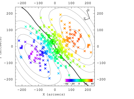
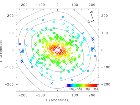
Figure 9.— Smoothed velocity field of PNe in NGC 3379, with the photometric major axis (PA=70^∘) oriented in the $x$-direction. Upper: Mean velocity field, with individual PN velocities plotted as crosses: see shaded bar for velocity scale. Iso-velocity contours are also plotted, with the heavy contour at zero velocity and subsequent contours at 10  km s^-1 intervals. Lower: Dispersion (rms velocity) field. Again, the bar shows the scale, and the contours run inwards from 60  km s^-1 to 180  km s^-1

7.2. Rotation

The most dramatic feature in Figure 9 is the clear rotation of the system, which is non-zero at a significance level of 3-$\sigma$. The projected rotation axis lies at a position angle of $\phi_{0}\sim 20^{\circ}$ east from north. This does not align with either the photometric major axis ($\sim 70^{\circ}$) or the photometric minor axis ($\sim-20^{\circ}$), implying that the galaxy cannot be a simple axisymmetric system. We note that the precise value of $\phi_{0}$ from our data is somewhat uncertain, because systematic offsets in our PN velocities are of order $\sim 20$ km/s, about half of the rotation amplitude in Figure 9. However, further indication of the galaxy’s triaxial nature comes from matching these kinematics to the absorption-line data at small radii, where the projected rotation axis is found to be $\sim-15^{\circ}$ (Statler & Smecker-Hane, 1999); such a twist in the rotation axis cannot occur in an axisymmetric system.

To better quantify this rotation, we have fitted the raw PN velocities with a simple rotation curve model,

$$v(\phi)=v_{0}\times\sin(\phi-\phi_{0}),$$ (5)

where $\phi$ is the position angle of the PN on the sky as measured from the center of NGC 3379, and the constants $v_{0}$ and $\phi_{0}$ respectively measure the amplitude of rotation and its projected axis. This fitting procedure has the advantage of being insensitive to the azimuthal completeness of the data; its applicability is discussed in Napolitano et al. (2001). The resulting best-fit parameters are $v_{0}=45\pm 15\,{\rm km}\,{\rm s}^{-1}$ and $\phi_{0}=20^{\circ}\pm 20^{\circ}$. We also looked for any indications of variation in these parameters with radius by dividing the data into three radial bins, but to within the errors the data are consistent with a flat rotation profile at a fixed position angle.

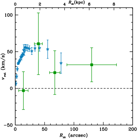
Figure 10.— Mean rotational velocity of stars and PNe along the major axis of NGC 3379. Boxes show PN.S data and stars show absorption-line kinematics from Statler & Smecker-Hane (1999).

We can also construct a more conventional major-axis rotation profile, for direct comparison with the major-axis long-slit absorption-line data. Figure 10 shows the results obtained by combining the PN data from a strip 50^′′ wide aligned with the photometric major axis, and mirrored through the center of the galaxy to double the sample size. The figure also shows the corresponding absorption-line data from Statler & Smecker-Hane (1999): in the central bin, the PN velocities are suppressed because the wide strip samples a long way up the minor axis of the galaxy, but at larger radii the amplitude of rotation is entirely consistent between PN.S and absorption-line data. It is also interesting to note that these data show no indication of the high rotation velocity predicted in the outer parts of elliptical galaxies by merger scenarios (Weil & Hernquist, 1996), although in any individual case such as this it is always possible that most of the rotation lies undetectably in the plane of the sky.

7.3. Velocity Dispersion Profile

It is apparent from inspection of Figure 9 that random motions dominate over the mean streaming motions throughout NGC 3379, so by accurately characterizing the random velocities we will capture most of the dynamical information that these data contain. Further, it is clear from Figure 9 that the velocity dispersion field is regular in appearance, and roughly aligned with the stellar isophotes. We can therefore characterize these random motions quite accurately with a simple azimuthally-averaged one-dimensional profile as a function of the intermediate axis radius, $R_{m}$.

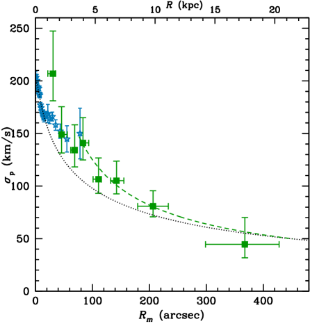
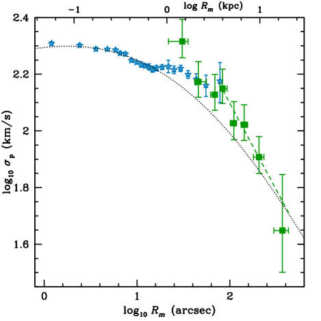
Figure 11.— Projected velocity dispersion profile for NGC 3379, showing data from stars (stars) and PNe (boxes), plotted on both linear (upper figure) and logarithmic axes (lower figure). Dashed lines show a power-law fit at large radii, while dotted lines show an isotropic constant mass-to-light ratio model.

As described in §6.2, we have calculated the empirical binned PN velocity dispersion profile, which we combine with the stellar absorption line data of Statler & Smecker-Hane (1999), presenting the result in Figure 11. The most striking feature of this plot is the rapid decline in the velocity dispersion with radius. A maximum-likelihood fit to the unbinned data at radii $R_{m}>80^{\prime\prime}$ (see below) gives a best-fit power law with an index of $-0.6\pm 0.2$. A possible concern is that the profile might be sensitive to the manner in which PNe have been flagged as contaminating objects in the tails of the distribution by the friendless algorithm (see §5.3): if the velocity distribution is significantly non-Gaussian at large radii, this algorithm could be overzealous in trimming objects from the tails of the distribution, systematically underestimating the true velocity dispersion. We have investigated this effect by constructing the dispersion profile after applying a more conservative application of the friendless algorithm that only truncates the velocity distribution at $5\sigma$, but find the difference to be insignificant. Thus, the decline in velocity dispersion with radius does not appear to be an artifact arising from the assignment of galaxy membership. In what follows we will apply the more usual $3\sigma$ cut, and PNe lying beyond this cut will no longer be plotted. This proximity in the slope of the velocity dispersion profile to the Keplerian value of $-0.5$ has been seen repeatedly in earlier PN data for NGC 3379 (Ciardullo et al. (1993), R+03, Sluis & Williams (2006)), but is extended by the new data set to even larger radii. Since at these radii we are well outside most of the luminous component of the galaxy, it acts very much like a point-mass potential, so the simplest interpretation of the Keplerian decline is that the mass is dominated by the luminous component and that we are seeing close-to-Keplerian isotropic orbits in its potential. However, as discussed in the Introduction, there is always the possibility that a more complex orbit distribution could mimic this behavior in a different gravitational potential. Indeed, it is apparent from Figure 11 that there is a fair amount of structure in the velocity dispersion profile, including a rapid transition from a shallow inner slope to a steep outer slope at a radius of $\sim 80^{\prime\prime}$. Due to the long-range nature of the gravitational force, such rapid changes are difficult to induce by varying the gravitational potential, which at least suggests that a transition in the orbital structure of the galaxy is occurring.

7.4. Higher-Order Velocity Moments

One clue as to the true nature of the orbital structure is provided by higher order velocity moments. In particular, the fourth moment, usually presented as the non-dimensional kurtosis, $\kappa\equiv\langle v^{4}\rangle/\langle v^{2}\rangle^{2}-3$, offers a useful diagnostic. In systems where the orbits are preferentially circular, the observed line-of-sight velocities tend to pile up at the circular speed, in extreme cases producing a line-of-sight velocity distribution with two peaks at the positive and negative circular speed. Such distributions are characterized by negative values of $\kappa$. Conversely, a system containing objects on radial orbits will tend to produce a centrally peaked line-of-sight velocity distribution with long tails, resulting in a positive value of $\kappa$. The halo of a galaxy with isotropic orbits and a constant circular-velocity curve (i.e. with a massive dark-matter halo) has a Gaussian line-of-sight velocity distribution, and $\kappa=0$ (Gerhard, 1993).

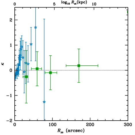
Figure 12.— NGC 3379 projected kurtosis profile, showing data from stars (stars) and PNe (squares).

We have therefore calculated the $\kappa$ profile for the PNe in NGC 3379, with the results presented in Figure 12. The figure also shows the higher-order moments obtained from the absorption-line spectra of Statler & Smecker-Hane (1999): they obtained the related Gauss-Hermite coefficient $h_{4}$ (van der Marel & Franx, 1993; Gerhard, 1993), which we have transformed into the kurtosis by the approximate relation $\kappa\simeq 8\sqrt{6}h_{4}$.

The stellar kurtosis in Figure 12 shows significant departures from zero, which may reflect structural transition regions in the galaxy’s central parts, or systematic observational uncertainties (Bender et al., 1994). We are most concerned with the kurtosis of the PNe in the halo, where we might see a signature of radially-biased orbits (see §1). As seen in Figure 12, here the kurtosis is consistent with zero out to $\sim 200^{\prime\prime}$ or $\sim 4$$R_{\rm eff}$ (outside this radius, the small number of data points make the kurtosis measurement unstable). The PN data therefore rule out the more pathological models of extreme radial or tangential orbit distributions, but the constraint is still too weak to directly preclude a massive dark matter halo with mild radial anisotropy. Stronger constraints can be made with sophisticated full orbit modeling techniques as undertaken by R+03, incorporating the information from the shape of the velocity distribution in a more robust way than is possible with binned moments.

8. Dynamical Models

A full analysis of the dynamics of NGC 3379 is beyond the scope of this paper, but we can obtain some insights, and hopefully move toward resolving the issue regarding the presence or otherwise of a dark halo, by a fairly simple spherically-symmetric Jeans-based analysis.

8.1. Is A Spherical Model Reasonable?

The assumption of spherical symmetry does not seem an unreasonable proposition given NGC 3379’s approximately circular appearance, and we can always modestly transform projected coordinates into an exactly circularly-symmetric approximation by mapping all quantities along isophote contours to the intermediate axis radius, $R_{m}\equiv\sqrt{ab}=a\sqrt{1-\epsilon}$. However, there is of course no guarantee that a roughly circular object is intrinsically close to spherical, since it could be axisymmetric and viewed along the axis of symmetry, or even have a more complex three-dimensional shape.

Even with this imponderable, we can make a probabilistic estimate of the galaxy’s three-dimensional stellar ellipticity, $\epsilon_{\rho}$, based on the known properties of the general population of elliptical galaxies. Given an observed projected axis ratio $q_{I}$, we can find the probability of the intrinsic short axis ratio $q_{\rho}$ via:

$$P(q_{\rho}|q_{I})\propto P(q_{\rho})P(q_{I}|q_{\rho}),$$ (6)

where the distribution of galaxies’ intrinsic axis ratios, $P(q_{\rho})$, has been estimated by Lambas et al. (1992). If we assume an oblate galaxy, then we also know that

$$P(q_{I}|q_{\rho})\propto\frac{q_{I}}{\sqrt{(1-q_{\rho}^{2})(q_{I}^{2}-q_{\rho}^{2})}}$$ (7)

(Binney & Merrifield, 1998, equations 4.30 and 4.32), and so can solve for the posterior probability distribution. Given the observed value $q_{I}=0.84$ for NGC 3379, the median value of the resulting axis-ratio distribution is $q_{\rho}\approx 0.7$. If we relax the assumption of oblateness to a more realistic triaxial distribution, the median $q_{\rho}$ becomes even larger, so we can say that it is odds-on that the intrinsic ellipticity of the NGC 3379 stellar density distribution is less than 0.3. Assuming any additional mass contributed by dark matter is at least this close to spherical, this measurement then places an upper limit on the ellipticity of the total density. Further, the gravitational potential is always rounder than the mass distribution that generates it, so in this case we obtain an upper limit on the potential axis ratio of $\sim 0.1$ and we expect the spherical approximation to be good to $\sim$10% (Kronawitter et al., 2000). Of course this calculation is probabilistic in nature, and we could just be unlucky to find a highly aspherical galaxy projected as round on the sky, but we have at least demonstrated that a spherical model is a plausible place to start.

We therefore proceed to analyze the dynamics of this system assuming spherical symmetry. Under this assumption, the Jeans equation relating velocity dispersion to the mass distribution can be written in the compact form

$${GM(r)\over r}=v_{\rm c}^{2}(r)=\left[\alpha(r)+\gamma(r)-2\beta(r)\right]\sigma_{r}^{2}(r),$$ (8)

where $M(r)$ is the mass contained within radius $r$, which can be transformed into the circular speed $v_{\rm c}$. On the right-hand side, $\alpha$ is the logarithmic gradient of the tracer population density $j(r)$, (here the PNe), $\alpha\equiv-d\ln j/d\ln r$, $\gamma$ is the logarithmic gradient of the radial mean-square velocity, $\gamma\equiv-d\ln\sigma_{r}^{2}/d\ln r$, and $\beta$ is the usual anisotropy parameter,

$$\beta\equiv 1-\sigma^{2}_{\theta}/\sigma^{2}_{r},$$ (9)

defined such that isotropic systems have $\beta=0$, radially-biased systems have $\beta>0$, and tangential bias gives $\beta<0$. The tangential mean-square velocity, $\sigma^{2}_{\theta}$, contains both the mean streaming and random component, as set out in §6.2. However, since we saw in §7 that the random motions dominate everywhere, it can loosely be thought of as just the random component.

Although equation 8 looks simple enough, the large number of unknown functions means that it is far from trivial to solve. The only quantity that we can disentangle from the dynamical terms is $\alpha(r)$, since this is given fairly directly by the observed spatial distribution of the tracer population. We therefore deal with this term first, before returning to the more general solution of equation 8.

8.2. The Spatial Distribution of the Kinematic Tracer

As we saw in Figure 6, the projected light distribution of both stars and PNe is well represented by a Sersic (1968) law fit to the surface brightness (measured in magnitudes per square arcsecond^-2),

$$\mu(R)-\mu(0)\propto(R/a_{s})^{1/m}.$$ (10)

The best-fit parameters for this system are $m=4.74$, $a_{S}=0.0013^{\prime\prime}$, and a central surface brightness of $\mu_{0}=12.2\,{\rm mag}\,{\rm arcsec}^{-2}$ in the $B$-band. This fit breaks down in the innermost arcsecond of NGC 3379, but it is entirely adequate for the large-scale modeling purposes of this analysis (see Figure 6). After allowing for a Galactic extinction of $A_{B}=0.105$ (Schlegel et al., 1998), the model fit integrates to yield a total absolute magnitude of $M_{B}=-19.8$. The scale parameter can also be transformed into an estimate of the effective radius of $R_{\rm S,eff}=47^{\prime\prime}$, a value which is used throughout this paper. As an aside, we note that this value does not match very well with the more usually adopted value of $R_{\rm eff}$= 35.5^′′ (Peletier et al., 1990) but also that none of the analysis here depends on the value adopted. The observed light distribution of equation 10 deprojects to a luminosity density of

$$j(r)\propto(r/a_{\rm S})^{-p}\exp{[-(r/a_{\rm S})^{1/m}]},$$ (11)

where $p$ is a known function of $m$ (Prugniel & Simien, 1997), and we can then readily calculate the logarithmic radial gradient of this quantity as a function of radius, $\alpha(r)$, or integrate it out in radius to obtain the luminosity contained within radius $r$, $L(r)$. This quantity can then be compared to the enclosed mass at any radius via the mass-to-light ratio, $\Upsilon(<r)=M(r)/L(r)$.

We can also calculate the contribution from the stars themselves to $M(r)$ if we know the mass-to-light ratio of the stellar population, $\Upsilon_{*}$, which allows us to convert the luminosity density into the stars’ contribution to the total mass density, $\rho_{*}(r)=\Upsilon_{*}\times j(r)$. The appropriate value for the stellar mass-to-light ratio of NGC 3379 has been studied in some detail by Cappellari et al. (2006), who used some of the latest stellar population synthesis models to match the observed spectrum of the galaxy to a credible stellar population, and hence infer its mass. From this analysis, the conversion from $B$-band luminosity density into stellar mass density is

$$\Upsilon_{*,B}=(7.3\pm 0.7)\Upsilon_{\odot,B},$$ (12)

where $\Upsilon_{\odot,B}$ is the mass-to-light ratio for the Sun in this band. One uncertainty in any such calculation is the form of the stellar mass function, since it is always possible to hide mass in the form of copious low-mass stars that contribute little to the total luminosity. The calculation by Cappellari et al. (2006) was based on the current best estimate for this mass function from Kroupa (2001), but it is worth noting that the adoption of the traditional Salpeter (1955) mass function raises the mass-to-light ratio by $\sim 30\%$, so the value in equation 12 is if anything a lower bound on the stellar mass-to-light ratio.

8.3. Solving the Jeans Equation

At this point, there are several ways of confronting equation 8 with the kinematic data to try to infer something about the dynamics of the tracer population and the potential within which it orbits. The most straightforward approach is to assume a model for both the mass distribution $M(r)$ and the anisotropy of the orbits, $\beta(r)$, and solve the equation for $\sigma(r)$. Both components of the velocity dispersion are then specified through equation 9, and we can project these dynamics back onto the sky for comparison with the observed velocity dispersion profile.

Given the near-Keplerian decline discussed in §7.3, and the extensive argument over whether or not NGC 3379 has a massive halo, the obvious place to start is with the simplest plausible model in which the mass follows the tracer population and the orbits are isotropic ($\beta\equiv 0$). There is only one free parameter in this model, the constant mass-to-light ratio $\Upsilon$, which we can determine by normalizing the predicted velocity dispersion profile to the observed one. Since this model is most credible as an approximation at small radii, where everyone agrees that the luminous component is more likely to dominate the mass, we have carried out this normalization over of the range $2^{\prime\prime}<R<15^{\prime\prime}$. The resulting model line-of-sight velocity dispersion profile (making use of formulae in MŁ05) is reproduced in Figure 11. In the central region, the fit to the observed velocity dispersion is very good, suggesting that this model is a satisfactory description of the inner parts of NGC 3379; indeed, previous analyses of the kinematics of the central part of NGC 3379 have consistently found that it can be modeled in this simple way (Kronawitter et al., 2000; Gebhardt et al., 2000; Cappellari et al., 2006). The normalization implies a central mass-to-light ratio relative to Solar in the $B$-band of $\Upsilon_{B}=6.3\Upsilon_{\odot,B}$. Comparing this value to the contribution from the stellar component, equation 12, it is clear that most, if not all, of the mass at these radii can be attributed to the stars; if we want clear evidence of dark matter, we will have to look further out in the galaxy.

Indeed, at larger radii in Figure 11 it is apparent that this simple model and the velocity dispersion data differ, due to the changes in slope in the velocity dispersion profile commented upon in §7.3. To try to understand the significance of this structure in the profile, we next consider a simple phenomenological model for the intrinsic velocity dispersion profile,

$$\sigma_{r}=\sigma_{0}\left(\frac{r}{r_{0}}\right)^{-\delta}\left[1+\left(\frac{r}{r_{0}}\right)^{\eta}\right]^{-1}.$$ (13)

This model is not motivated by any prejudice as to the mass distribution, but simply as an attempt to reproduce the observed change in logarithmic slope of the velocity dispersion at large radii. Once we have adopted a functional form for $\beta(r)$, the velocity dispersion is fully specified, and we can project the model for comparison with the line-of-sight velocity dispersion data. By iteratively adjusting the free parameters in equation 13, $\{\sigma_{0},r_{0},\eta,\delta\}$, the model can then be fitted to the observed profile. Since we are primarily interested in explaining the large-scale change in the slope of this profile, and not the detailed structure at intermediate radii, we only fit to the data at $R<8^{\prime\prime}$ and at $R>40^{\prime\prime}$. Once we have such a model that fits the kinematic data, we can solve equation 8 for $M(r)$, and hence calculate the enclosed mass-to-light ratio as a function of radius.

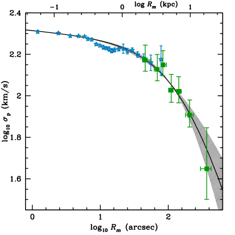
Figure 13.— Phenomenological fit to the NGC 3379 velocity dispersion data using the model of equation 13 assuming $\beta\equiv 0$. The line shows the best fit and the shaded region shows the range covered by acceptable fits.

Again, we start with the simplest possibility of an isotropic galaxy with $\beta\equiv 0$. As Figure 13 shows, the model can reproduce the observed velocity dispersion data very well over the fitted radial range. Obviously the data do not uniquely specify the model parameters, but, as the shaded region shows, the acceptable fits capture the range of possible smoothly-varying dispersion profiles fairly comprehensively.

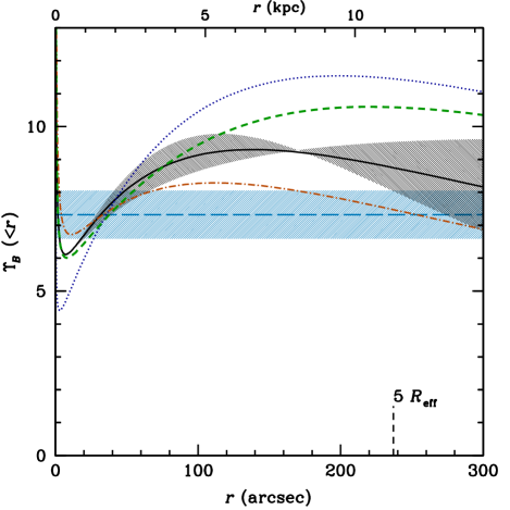
Figure 14.— Cumulative mass-to-light ratio profiles obtained by solving the Jeans equation using the phenomenological velocity dispersion model of equation 13. The solid line and shaded region show the best fit and the acceptable range of values derived from the fits in Figure 13 for an isotropic model; the dotted line shows the best-fit radially-biased model; the dot-dash line shows the best-fit tangentially-biased model; and the short-dashed line shows the best-fit variable-anisotropy model. The long-dashed line and surrounding shaded error region show the stellar mass-to-light ratio.

The result of inserting this model in equation 8 and solving for $\Upsilon_{B}(<r)$ is shown in Figure 14. The figure also shows the mass-to-light ratio of the stellar population from equation 12. As qualitatively predicted, the enhanced velocity dispersion at large radii translates into an increasing mass-to-light ratio, but the effect is far from dramatic. The PN data become very sparse outside $240^{\prime\prime}$ (5$R_{\rm eff}$), so if we adopt this as a benchmark value, we find that the mass-to-light ratio within this radius is $\Upsilon_{{\rm 5},B}=8.7^{+0.8}_{-0.7}$ $\Upsilon_{\odot,B}$. Given the value for the stellar component from equation 12, we thus infer a dark matter fraction within this radius of between 5% and 30%.

To this point, we have imposed the constraint of isotropy on the orbits, and clearly if we relax this imposition then the limits on the dark matter fraction will become even weaker. Simulations and the weak limits imposed by the higher order moments discussed in §7.4 suggest that plausible limits on the anisotropy parameter are $-0.5<\beta<0.5$, so as a simple first test of relaxing the orbital constraint we have repeated the above analysis using the extrema of this distribution. As the famous degeneracy between $\beta(r)$ and $M(r)$ would imply, models with $\beta=\pm 0.5$ can reproduce the observed velocity dispersion profile with the same accuracy that we saw for the isotropic model of Figure 13. When the best-fit models are then passed through the Jeans equation to solve for the mass-to-light ratio, we see the impact of anisotropy. As shown in Figure 14, the effects of varying the anisotropy in this way dominate the statistical uncertainty from the range of models that fit the data for a given anisotropy. At our benchmark radius of 5$R_{\rm eff}$, the permitted range of mass-to-light ratios is $\Upsilon_{{\rm 5},B}=6.8-12.2\Upsilon_{\odot,B}$, implying an enclosed dark matter fraction of somewhere between none and 45%, which is still on the low side – simple $\Lambda$CDM-based models suggest that the value at these radii should be around 60% (Napolitano et al., 2005).

Clearly, we could play the game of adopting ever more complicated models for $\sigma_{r}(r)$ and $\beta(r)$ to try and fit every observed feature, but the simplified nature of this entire spherical Jeans-based analysis means that we are unlikely to learn much more. However, as one final embellishment, we consider a model in which the orbits are isotropic at small radii, but undergo a transition to a radial bias at large radii. Such an arrangement was the principal suggestion made by D+05 to explain the declining velocity dispersion in NGC 3379, and, as discussed in §7.3, is hinted at by the data themselves, as the dispersion profile in Figure 11 seems to undergo a transition between slopes at a radius of $\sim 70^{\prime\prime}$. To model this arrangement, we adopt the functional form used by MŁ05 of

$$\beta(r)={0.5r\over r+r_{\rm a}},$$ (14)

where $r_{\rm a}\simeq 1.4$ $R_{\rm eff}$  $\simeq 65$”. The Jeans analysis result from this anisotropy function is also plotted in Figure 14. Perhaps unsurprisingly, this result lies somewhere between the isotropic case and the $\beta=0.5$ case. It implies a mass-to-light ratio within the benchmark radius of $\Upsilon_{{\rm 5},B}\simeq 10.6\Upsilon_{\odot,B}$, corresponding to a dark matter fraction of $\simeq 30\%$. Again, there is evidence for dark matter, but not the dominant amount that $\Lambda$CDM models predict. It also conflicts with the results from the D+05 simulations that motivated it, which have a dark matter fraction within this radius of $\simeq 60\%$. We return to this discrepancy in §9.

8.4. Comparison to Previous Data Modeling

Before we look at the apparent conflict between mass models motivated by simulations and those that result from the analysis of real data, it makes sense to look a little more closely at the credibility of the data modeling. In particular, it is useful to explore how reliably different analyses reproduce the same answers, and how consistent the results obtained from different types of data are.

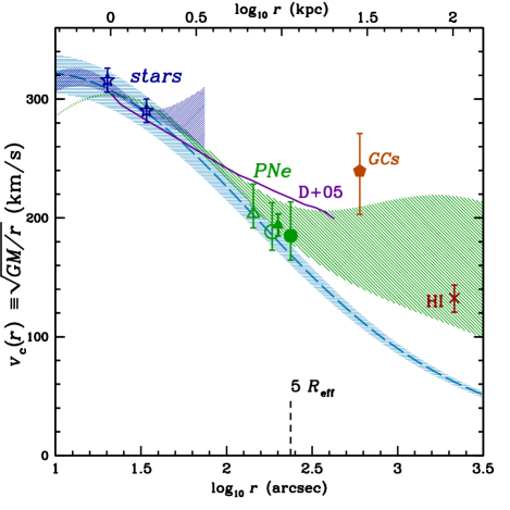
Figure 15.— Summary of models determining the NGC 3379 circular velocity profile. From stellar absorption-line data, axisymmetric three integral models from Shapiro et al. (2006) and Gebhardt et al. (2000) are shown as stars, and the range of spherical models determined by Kronawitter et al. (2000) based on distribution functions is shown as the inner shaded region. Previous results from Jeans analyses of PNe are shown as a filled triangle (Ciardullo et al., 1993), an open circle (R+03), and an open triangle (Sluis & Williams, 2006). A combined orbit-model fit to PNe and stellar data (R+03) is shown as the extended shaded region. A globular cluster result from Bergond et al. (2006) and the HI circular speed from Schneider (1985) are also shown. The result from this paper is shown as a filled circle. The dashed line and surrounding shaded error region shows the contribution to the circular velocity from the stellar component. The solid line shows the average result from the simulations of Dekel et al. (2005).

A summary of the available stellar-kinematic mass modeling for NGC 3379 is provided in Figure 15, where we have transformed the enclosed mass into a circular speed for more direct comparison with the rotation curves of spiral galaxies, and as a quantity independent of the distance and luminosity model. As the caption describes, this figure shows the results from stellar absorption-line data at small radii and those obtained from PNe at larger radii, as well as the combined analysis of both types of data by R+03.

We have also plotted the recent globular cluster enclosed mass estimate from Bergond et al. (2006). Since the globular cluster population is more extended than the stellar component, it offers a probe of the enclosed mass at even larger radii. Unfortunately, however, NGC 3379 has a fairly meager population of globular clusters, so the statistics are not yet good, making it impossible to disentangle mass effects from orbital anisotropy (which could be completely different from the anisotropy in the stellar orbits). Further, the more extended nature of their distribution and the small numbers available mean that it may be difficult to decontaminate the sample of interloping NGC 3384 clusters.

One further mass probe at even greater distances is provided by the kinematics of the rotating ring of HI that is seen to surround this galaxy at a radius of $\sim 100\,{\rm kpc}$ (Schneider, 1985). Again, NGC 3384 confuses the issue somewhat since this ring encompasses it as well as NGC 3379. However, if we adopt the simplest approach of dividing the mass between the two galaxies in the same ratio as their luminosities, attributing two thirds of the mass to NGC 3379, we finally obtain the outermost point shown in Figure 15. What is most striking about this plot is the consistency of the results. When different observations of the same tracer are employed, the results are very similar. Equally, when data sets are analyzed using different methods, be they Jeans analysis, distribution function fitting or combining a library of orbits, or making different assumptions about the symmetry of the galaxy, very comparable results are obtained. When completely different tracers are employed, the results still match up to within the respective errors. Ultimately, all these experiments agree that although there is strong evidence for dark matter on the largest scales, within the benchmark radius of 5$R_{\rm eff}$ the circular velocity curve is well matched to that inferred from the stellar component alone (also shown in Figure 15), so the amount of dark matter there is at most modest.

9. Scantily-Clad or Fully-Clothed?

The relative consistency of the various models derived from kinematic data returns us to the question of why the conclusion from these studies differs so significantly from that reached by working in the opposite direction of generating “observations” from simulations, and comparing them to the data. Specifically, D+05 claimed that they were able to reproduce the earlier PN.S results on the velocity dispersion profile by “observing” a simulated galaxy merger that took place in the framework of standard $\Lambda$CDM dark matter halos. This contrasts with the findings of R+03 and Napolitano et al. (2005) that the data were not consistent with $\Lambda$CDM halos.

D+05 concluded that three factors were responsible for the discrepancy:

1. Stars are thrown into radial halo orbits during the merger process.

2. The triaxial nature of the galaxies can depress $\sigma_{\rm p}$ at some viewing angles.

3. The PNe trace young stars formed in the merger rather than the old stars usually assumed.

We therefore consider these possibilities in turn.

The first factor seems plausible, since any stars thrown out from near the centre of a galaxy in a merger process must end up on fairly radial orbits. Indeed, it seems to be a generic expectation for galaxy halos (Diemand et al., 2005; Abadi et al., 2006; Hansen & Moore, 2006), although there are some dissenting views on even this basic point (González-García & Balcells, 2005; Athanassoula, 2005). However, it is certainly not the explanation for the discrepancy between the simulations and the data-fitting results, as this possibility has been fully incorporated in the data fitting process of R+03. In fact, the anisotropy profile $\beta(r)$ found in this way was very similar to that of the simulations. So there is something else at work here besides the obvious effects of radial anisotropy.

The second factor, a possible unfavorable viewing angle for NGC 3379, is harder to rule out on the basis of observations of a single object. Indeed, it is known that a flattened system viewed face on will have its mass systematically underestimated if it is assumed to be spherical (Magorrian & Ballantyne, 2001). However, similar results were discussed by R+03 in three other galaxies (NGC 821, 4494, and 4697). We would have to be very unlucky for all these systems to be face-on, especially since some of them appear significantly flattened on the sky.

The final factor invoked by D+05 also does not seem particularly plausible. Although there is a prediction that the bright end of the PNLF is populated by younger stars (Marigo et al., 2004), and one claim of the detection of such a system (Sambhus et al., 2006), this phenomenon has not been seen elsewhere. This lack of variation is particularly definitive in the best-studied case of our neighboring spiral M31 where one might expect recent star formation events to produce dramatic variations in the PN properties, yet no differences at all are found in the bright end cut-off of the PN luminosity function even when comparing the properties of bulge and disk populations at the level of subtlety afforded by a sample of almost 2800 PNe (Merrett et al., 2006). The apparent universality of the PN luminosity function in stellar populations of all ages is completely inexplicable if the bright end of this function is only populated where there are relatively young stars.

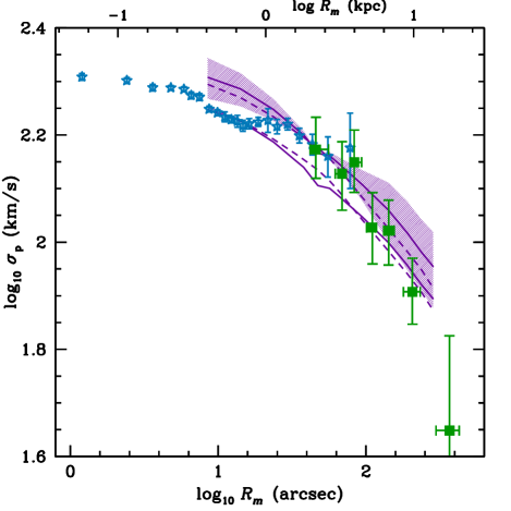
Figure 16.— Comparisons of projected velocity dispersion profiles between observations and Dekel et al. (2005) galaxy simulations. Symbols are as in Figure 11, with the addition of a solid line showing the dispersion profile of the old stars in the simulation, and a dashed line showing the profile for the young stars. Two possible normalizations are shown for each component. The shaded area illustrates the region of scatter for one case.

So, if none of these explanations holds water, why do the conclusions derived from simulations differ so dramatically from those presented here? One issue is that the simulations do not reproduce the observations as unambiguously as one might want, and that there is significant uncertainty as to how the simulation should be normalized to best match the data. Figure 16 compares the simulation’s velocity dispersion profile to that of the data. It is apparent from this figure that the over-all slope of the simulation’s profile does not match the data particularly well: the power-law index for the outer parts of the simulation lies in the range 0.2 – 0.4, as compared to the value of 0.4 – 0.8 that we found for the data in §7.3. The match is a bit better to just the young stars in the simulation, but, as discussed above, it is difficult to see why the detected PNe should be associated with such a sub-population. Even where there is a crude match to the slope of the profile, the simulations do not reproduce the structure seen in the data, so there is an ambiguity in the velocity normalization depending on the radius at which one chooses to match the two, as Figure 16 illustrates. This uncertainty is compounded by the fact that there is a similar ambiguity in the normalization of simulation and data in the spatial coordinate as well: as was mentioned in §8.2, the observational measurement of NGC 3379’s effective radius can depend significantly on the manner in which it is determined. Coupling this uncertainty with the systematically different way in which $R_{\rm eff}$ was determined from the simulations (based on the radius within which half the mass is projected) means that matching the spatial scale of the simulation to the data generates an additional significant source of uncertainty.

The differences between the simulations and NGC 3379 extend beyond the kinematics. We note that the D+05 simulations contain a central blue “hump” in the stellar population (D+05 Figure 2a) that is not seen in NGC 3379. This phenomenon arises from the well-documented problem of the over-collapse of baryons in simulations of gas-rich mergers (e.g., Meza et al., 2003). Although D+05 state that their results are unaffected by this feature, it does raise a concern as to what subtler phenomena the simulation might also be failing to match. Since these systematically-incorrect gas dynamics will very strongly affect the motions of any new stars that form, it adds a further question mark to any conclusions based just on the young star population, although, as extensively discussed, there are already many question marks hanging over the association of the detected PNe with such a population. Additionally, this extra light adds an extra uncertainty in matching up the observed photometry to that of the simulation, compounding the issue associated with matching the spatial scales of the two. And finally, dissipation in mergers is strongly linked to the radius and velocity dispersion of the remnant’s center (Cox et al., 2006), so inaccuracies in this arena could very well lead to errors in the slope of the dispersion profile.

Not withstanding these problems in matching the simulations to the NGC 3379 data, we can still make a direct comparison between the mass profile results of R+03 and of D+05 (Fig. 15). Although the relative normalization is ambiguous, one can obtain a reasonably close match, given the run-to-run scatter of the simulations. So if the total mass profiles of R+03 and D+05 are not so different, why do the conclusions about dark matter differ? The answer lies in the decomposition of the total mass profile into stellar and dark matter components. As Figure 17 shows, the dark matter fraction in the simulations differs by more than a factor of two from that inferred from the data over a wide range of radii, and requires that the galaxy have a sizeable ($\sim 20$%) dark matter fraction at even the smallest radii. This discrepancy can be largely traced to the different values adopted for the $B$-band stellar mass-to-light ratio, $\Upsilon_{*,B}$. In order to match up the inner rotation curve of the simulations to those derived from the data, we find that the simulations only work if $\Upsilon_{*,B}=4-5\,\Upsilon_{\odot,B}$. This value clearly attributes less mass to the stellar component (and hence more mass to the dark halo) than the value in equation 12 adopted in this paper, which was derived from stellar population synthesis results. Although the lower value is not completely implausible for this galaxy (Gerhard et al., 2001), it is not really satisfactory to assign a mass-to-light ratio in this ad hoc manner, and it is surely preferable to adopt an astrophysically-motivated and constrained estimate.

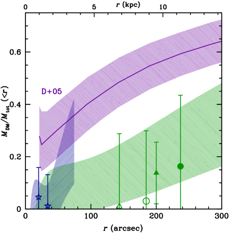
Figure 17.— The enclosed dark matter fraction as a function of radius for the D+05 simulations, compared to the results derived directly from observations of NGC 3379. Symbols for the data are as in Figure 15.

The bottom line here is that a significant conflict exists between the results derived from modelling the data directly and those obtained by matching the data to simulations, and it is not clear which analysis is flawed. The Jeans modeling has the advantage that, by construction, the data fit the model very well, but has the disadvantage that the model itself, with its imposed spherical symmetry and simple view of the tracer population, does not provide an entirely realistic picture of a galaxy. Conversely, the simulations are constructed to be as realistic as possible in describing the properties of a galaxy, but then are not designed to reproduce any particular galaxy with great accuracy. Ultimately, the solution must be to keep working from both directions, producing more sophisticated dynamical models from the data and putting better physics into a broader suite of simulations to match the properties of particular systems. Until these processes meet somewhere in the middle, we really will not be able to say definitively whether NGC 3379 is as lacking in dark matter as the modeling of this paper suggests, or whether it has the ample dark-matter clothing that D+05 found in their simulations.

10. Summary and Outlook

This paper presents the first fully-processed results from the PN.S survey of nearby ordinary elliptical galaxies, which has yielded a catalog of 191 PNe in NGC 3379. The data processing is discussed in detail. Given the novel nature of the instrument, we have gone into the description of the data processing in some detail. Comparison with existing smaller data sets has confirmed that the resulting kinematic measurements have velocity errors well within what is required for studying the large-scale dynamics of elliptical galaxies. The data on NGC 3379 have allowed us to study the kinematics of this galaxy out to almost ten effective radii. We detect a small amount of rotation, but random motions dominate throughout, the velocity dispersion showing the regular pattern expected for a near-spherical galaxy. There is no evidence for the large amounts of angular momentum stored in rotation at large radii that are predicted by merger simulations of elliptical formation.

We are able to confirm and extend the previous findings that the velocity dispersion falls with radius in a near-Keplerian manner. A spherical Jeans model confirms that an isotropic model with a modest amount of dark matter at large radii can fit the data very well. These results are found to be consistent with previous studies of the stellar and PN kinematics of the galaxy, and also fit reasonably well with the mass inferred from other tracers. The amount of dark matter is low compared to the predictions of $\Lambda$CDM, and, contrary to previous claims, this discrepancy cannot be resolved simply by changing the orbital anisotropy of the tracer population.

Our results continue to conflict with those found through comparison with merger simulations by D+05, which claimed that the observed kinematics are consistent with the presence of a conventional dark halo around the galaxy. We have explored the various explanations that have been advanced to explain this discrepancy, but do not find any to be entirely convincing. Just as there are shortcomings in the spherical Jeans modeling of the data, so there are issues in matching a simulation to a specific galaxy, and it is not clear which is more likely to be in error. One interesting difference is that the D+05 model contains significant amounts of dark matter even at very small radii, whereas the Jeans-based models do not. We have traced much of this difference to the mass-to-light ratios adopted for the stellar component, which differ by almost a factor of two. We thus appear to be arriving at the same ambiguity that beset attempts to decompose rotation curves of spiral galaxies into luminous and dark components, in that the amount of mass to attribute to the stellar component was not well constrained. Although this issue remains a challenge, it is not necessarily insurmountable, and we hope to have made at least a first step toward addressing it by setting the mass-to-light ratio of the stellar component on the basis of astrophysically-motivated population synthesis models matched to the photometry of the individual galaxy, rather than leaving it as a variable parameter with which to re-enforce our prejudices.

In order to advance the data modelling approach to the study of elliptical galaxies, to try to reconcile the results with those from simulations, we propose to follow a two-pronged strategy. First, we intend to perform more sophisticated modeling of the data. By relaxing some of the constraints such as spherical symmetry, we will be able to see what effect these artificial limitations might be having on the inferences that we draw. Further, we can make more efficient use of the data than simply binning velocities to determine a dispersion profile: with more detailed analysis, we can use the complete projected phase space distribution, and can also extract the information in a manner that is more robust than taking moments. Second, we will carry out a comparable analysis on the other ordinary elliptical galaxies for which we are obtaining data with PN.S. By analyzing a broader sample in a coherent and consistent manner, we will be able to see just how common systems like NGC 3379 are, thus ruling out some of the less interesting explanations for its strange properties such as an unfortunate viewing angle. We will also be able to start to investigate how the large-scale dynamical properties of elliptical galaxies correlate with other factors such as their environment. Hopefully, this further work will answer unequivocally some of the fundamental questions that remain outstanding in the study of the most ordinary of elliptical galaxies.

References

- Abadi et al. (2006) Abadi, M. G., Navarro, J. F., & Steinmetz, M. 2006, MNRAS, 365, 747
- Arnaboldi et al. (1998) Arnaboldi, M., Freeman, K. C., Gerhard, O., Matthias, M., Kudritzki, R. P., Méndez, R. H., Capaccioli, M., & Ford, H. 1998, ApJ, 507, 759
- Athanassoula (2005) Athanassoula, E. 2005, in AIP Conf. Proc. 804: Planetary Nebulae as Astronomical Tools, ed. R. Szczerba, G. Stasinska, & S. K. Gorny, 333–340
- Bender et al. (1994) Bender, R., Saglia, R. P., & Gerhard, O. E. 1994, MNRAS, 269, 785
- Bergond et al. (2006) Bergond, G., Zepf, S. E., Romanowsky, A. J., Sharples, R. M., & Rhode, K. L. 2006, A&A, 448, 155
- Bertin & Arnouts (1996) Bertin, E., & Arnouts, S. 1996, A&AS, 117, 393
- Bertola et al. (1993) Bertola, F., Pizzella, A., Persic, M., & Salucci, P. 1993, ApJ, 416, L45
- Binney & Mamon (1982) Binney, J., & Mamon, G. A. 1982, MNRAS, 200, 361