High Resolution Molecular Gas Maps of M33

Abstract

New observations of CO ($J=1\to 0$) line emission from M33, using the 25 element BEARS focal plane array at the Nobeyama Radio Observatory 45-m telescope, in conjunction with existing maps from the BIMA interferometer and the FCRAO 14-m telescope, give the highest resolution ($13^{\prime\prime}$) and most sensitive ($\sigma_{rms}\sim 60$  mK) maps to date of the distribution of molecular gas in the central 5.5 kpc of the galaxy. A new catalog of giant molecular clouds (GMCs) has a completeness limit of $1.3\times 10^{5}$ $M_{\sun}$. The fraction of molecular gas found in GMCs is a strong function of radius in the galaxy, declining from 60% in the center to 20% at galactocentric radius $R_{gal}\approx 4$ kpc. Beyond that radius, GMCs are nearly absent, although molecular gas exists. Most (90%) of the emission from low mass clouds is found within 100 pc projected separation of a GMC. In an annulus $2.1<R_{gal}<4.1$  kpc, GMC masses follow a power law distribution with index $-2.1$. Inside that radius, the mass distribution is truncated, and clouds more massive than $8\times 10^{5}$ $M_{\sun}$ are absent. The cloud mass distribution shows no significant difference in the grand design spiral arms versus the interarm region. The CO surface brightness ratio for the arm to interarm regions is 1.5, typical of other flocculent galaxies.

1. Introduction

The nearby galaxy M33 is an ideal site to study molecular gas and star formation in the larger context of a disk galaxy. Most of our knowledge of star formation and molecular clouds is informed by nearby star forming regions such as Taurus and Orion, but studies of star formation across the Milky Way as a whole are confused by our perspective from within the Galactic disk. In contrast, the M33 disk face is visible ($i\approx 52^{\circ}$, Corbelli & Salucci, 2000), so it is easier to study molecular gas in relationship to other components of the galaxy. In addition, M33 is near enough ($D=840$ kpc, Freedman et al., 2001) that individual molecular clouds can be resolved with a large single-dish telescope or millimeter interferometer.

Because of the perspective that observations of M33 offer, the galaxy has been the target of many large-scale studies of molecular gas. Wilson & Scoville (1989) observed the inner region of the galaxy in CO ($J=1\to 0$) with the NRAO 12-m and followed up with high resolution observations using the Owens Valley interferometer (Wilson & Scoville, 1990). The high resolution observations were used to study the properties of individual molecular clouds and compare to clouds in the Milky Way. A further study (Wilson et al., 1997) took advantage of the disk visibility to study variations in the properties of molecular gas across a range of galactocentric radii. Following improvements in millimeter-wave instrumentation, large-scale surveys of the galaxy became possible, such as that of Engargiola et al. (2003, hereafter EPRB) who used the BIMA millimeter interferometer to identify all GMCs across the star forming disk. Rosolowsky et al. (2003) studied a limited area of the disk, comprising about 1/3 of the clouds in the BIMA survey, at higher resolution. The study determined individual cloud properties including virial masses, confirmed the work of Wilson & Scoville (1990), and constrained GMC formation mechanisms by comparing the predicted and observed values for GMC angular momentum. Finally, Heyer et al. (2004, hereafter HCSY) used the FCRAO 14-m to complete a single-dish survey of the entire galaxy. Comparison with IRAS data determined the local star formation rate as a function of the surface density of molecular gas.

The existing observations, while providing a wealth of data, also raise additional questions that merit another look at the molecular gas in M33. In particular, comparison of the interferometer-only study of EPRB with the single-dish survey of HCSY shows that the interferometer recovered only 20% of the CO flux in the galaxy! Because the typical size scales of molecular clouds in M33 should roughly match the synthesized beam of the interferometer, such a small fraction of flux recovery is unexpected. What is the nature of the remaining molecular gas? One clue comes from the steep mass distribution of GMCs in M33. Unlike the Milky Way, EPRB found that the mass distribution was “bottom heavy” i.e. most of the molecular mass was found in clouds near their sensitivity limit. Thus, it appears that most of the missing flux is comprised of low-mass molecular clouds that the interferometer could not detect. This prompts several questions about the nature of such clouds: Where are these low mass molecular clouds located relative to the GMCs? Does the fraction of material found in GMCs vary over the galaxy? These questions are not easily answered by the existing observations, because the diffuse, extended emission of the lower-mass clouds is not easily detected by a radio interferometer, and the existing single dish observations do not have the angular resolution to define individual clouds.

To study the distribution of low mass clouds in more detail, we mapped the inner 2 kpc of M33 using the BEARS receiver on the 45-m telescope at the Nobeyama Radio Observatory (NRO). The NRO 45-m data give better sensitivity than previous observations and allow detection of a greater fraction of the CO in the central region. We present two new maps: a BIMA+FCRAO map of the entire galaxy and a BIMA+FCRAO+NRO map of the inner 2 kpc. The maps are complementary — the first surveys the entire galaxy at $13^{\prime\prime}$ (50 pc) resolution, sufficient to identify individual GMCs, while the second has 50% better point source sensitivity and a factor of 3.5 better column density sensitivity, though having poorer resolution ($20^{\prime\prime}=75$ pc) and limited coverage. Section 2 of this paper describes the new observations at NRO, while §3 explains the data processing and production of the maps. Section 4 presents the new GMC catalog. The new catalog demonstrates significant variations in the mass distribution across the face of the galaxy, as described in §5. Section 6 summarizes the results.

2. Nobeyama Radio Observatory Observations

The BEARS array on the 45 m telescope at Nobeyama Radio Observatory consists of 25 SIS mixer receivers arranged in a $5\times 5$ array with 41$\farcs$1 between the elements (Sunada et al., 2000). With the $14^{\prime\prime}$ beam size at 115 GHz, the elements are separated by 3 resolution elements on the sky. The basic unit of the M33 observations consisted of nine separate pointings arranged in a $3\times 3$ grid, each offset from the previous by 14″. This strategy observes a $(3.5^{\prime})^{2}$ region at half-Nyquist sampling. To acquire fully sampled data, this observation must be repeated three additional times with a 7″ offset in each direction. Thus, a fully-sampled map consists of 900 individual pointings separated by $7^{\prime\prime}$; a half-sampled map contains 225 pointings separated by $14^{\prime\prime}$. The BEARS receiver requires using the 25-element autocorrelator array as a back end. It has a total bandwidth of 512 MHz split into 1024 channels, resulting in a nominal velocity resolution of 1.3 km s^-1 in the ¹²CO ($J=1\to 0$) line.

Figure 1.— M33 field locations observed with the NRO 45-m. The boundaries of the observed fields established by the 3.5^′ size of the BEARS receiver are indicated on an H$\alpha$ map of the galaxy Massey et al. (2006). Of the 14 fields shown, the six fields with grey borders were observed with full sampling and the remaining 8 fields were sampled half as densely. A dashed ellipse is drawn at $R_{gal}=2$ kpc, illustrating that the survey covers the galaxy out to this distance. Properties of the fields are given in Table 1.

The observation strategy divided M33 into $(3.5^{\prime})^{2}$ regions defined by the footprint of the receiver array on the sky. Figure 1 shows the fields observed, and Table 1 gives their positions. For each field observed with half-Nyquist sampling, we observed the nine individual position offsets in 20 second scans, then position switched to an absolute reference position. The reference positions were chosen to be H II regions at large galactocentric radius ($R_{gal}$). These regions may contain CO emission, but they were always chosen so that the velocity of any emission in the reference beam would be much different from the line velocity in the observation position. In good observing conditions, two scans could be obtained between reference positions. In marginal weather, the number of scans had to be decreased to one, and the reference position was an offset of $30^{\prime}$ in azimuth instead of an absolute position. One pass through the nine positions of a field took five to six minutes depending on the settle time for the telescope, and typical observations utilized 12 cycles obtaining 180 seconds of integration time at each position. This completed a half-Nyquist observation of a field in 90 minutes. Before and between each field, we updated the pointing solution for the telescope using the S40 receiver to observe SiO ($J=1\to 0,v=0,1$) maser emission from IRC+30021. In low wind conditions, the pointing solution drifted by $<5^{\prime\prime}$ over the hour required to observe a single field. When the wind velocity was steadily above 5 m s^-1, the pointing drift could exceed $10^{\prime\prime}$ over an hour.

Table 1NRO/BEARS Field Parameters

Field	Central Position	Scans	Frac. Retained	Sampling
1	01:33:34.4 +30:34:51.2	108	0.94	Half-Nyq.
2	01:33:34.4 +30:38:23.6	108	0.99	Half-Nyq.
3	01:33:34.4 +30:41:42.2	108	0.97	Half-Nyq.
4	01:33:34.4 +30:45:07.7	108	0.84	Half-Nyq.
5	01:33:50.9 +30:34:51.2	108	0.96	Half-Nyq.
6	01:33:50.9 +30:38:23.6	382	0.71	Nyquist
7	01:33:50.9 +30:41:42.2	324	0.84	Nyquist
8	01:33:50.9 +30:45:14.5	323	0.87	Nyquist
9	01:34:06.8 +30:34:51.2	112	0.95	Half-Nyq.
10	01:34:06.8 +30:38:23.6	436	0.73	Nyquist
11	01:34:06.8 +30:41:42.2	108	0.96	Half-Nyq.
12	01:34:06.8 +30:45:07.7	108	0.97	Half-Nyq.
13	01:34:06.8 +30:48:40.0	320	0.71	Nyquist
14	01:34:22.8 +30:48:40.0	163	0.46	Nyquist

We observed from 2005 February 9 to February 17 as long as M33 was at suitable elevation, excluding time lost to maintenance and bad weather. In that time, we completed observations of 14 of the $(3.5^{\prime})^{2}$; six fields are Nyquist sampled and the remaining eight fields are half-Nyquist sampled (see Figure 1 and Table 1 for details).

Since each element of the BEARS receiver consists of a double side band SIS receiver, we calibrated the array with observations using a single-sideband receiver to obtain an accurate intensity scale. At the latitude of the Nobeyama Radio Observatory, M33 transits above the elevation limit of the 45-m telescope ($80^{\circ}$) rendering it unobservable for 90 minutes in the middle of the observations. During that time we calibrated the efficiency of each pixel of the BEARS receiver by comparing observations of NGC 7538 ($\alpha_{2000}=23^{\mathrm{h}}11^{\mathrm{m}}45\fs 5$ ,$\delta_{2000}=+61^{\circ}28^{\prime}09^{\prime\prime}$) made with each element of the array to those made of the same position with the single-sideband S100 receiver. The intensity scaling factor for each BEARS pixel relative to the S100 receiver was the ratio of the integrated intensities in the respective observations. The BEARS spectra were multiplied by these scaling factors averaged over the course of the observing run. The scaling factors ranged from 1.7 to 3.6 with a median value of 2.4. Daily variation of the scaling factors was $\lesssim 20\%$ for all elements; this variation dominates the uncertainty in the overall flux calibration. This scaling places BEARS spectra onto the S100 intensity scale, and the spectra must be scaled up by a further factor of 2.56 ($=1/\eta_{mb}$) to correct for the main beam efficiency. With all corrections, the noise level of the final map is 85 mK on the $T_{A}^{*}$ scale.

3. Data Reduction

3.1. Nobeyama Radio Observatory Data

Inspection revealed several pathologies in the NRO/BEARS data. These are: (1) pointing errors induced by high wind speeds, (2) baseline variations, and (3) interloper signals in the base band. Because of the data volume — 62300 raw spectra — automated processing was needed to correct these problems. Scans taken when wind velocities exceeded 7.5 m s^-1 were rejected in their entirety. Spectral baselines were established for every spectrum by a fourth-order b-spline fit with break points established every 100 km s^-1, ignoring regions within 32 channels of the beginning and end of the spectrum, within 20 channels of a bad correlator section near channel 300, and within 30 km s^-1 of the H I line-of-sight velocity at observed and reference positions in M33. These exclusions prevented the routine from fitting a baseline to actual CO emission in M33. The baseline fit accounts for low-order baseline ripples of arbitrary shape but cannot account for high-order “standing wave” patterns in the resulting data caused by interloper signals in the base band. Spectra affected by such signals can be readily identified because the rms residual from the b-spline fit is dramatically larger than for the remainder of the observations. The small number of spectra for which the rms residual is 4 times the median were rejected. Table 1 reports the fraction of scans that remain after wind speed and baseline rejection. The acceptable spectra were Hanning smoothed and down-sampled to a final channel width of $2.6$ km s^-1 before being gridded into a data cube using a Gaussian smoothing kernel with a FWHM of $20^{\prime\prime}$.

3.2. Merging the Interferometer and Single Dish Maps

The first step in the analysis was to merge the FCRAO (HCSY) and BIMA (EPRB) data sets. As noted in §1, the interferometer map recovers only $\sim$ 20% of the flux found in the single-dish map, though the interferometer map detects nearly all the GMCs in the galaxy. The 14-m FCRAO dish recovers all flux at the small spatial frequencies not sampled by the BIMA observations, which have minimum baselines $\lesssim$ 7 m. Therefore, the two maps can be combined to produce a single high-resolution, fully-sampled map. The power in the overlapping range of spatial frequencies shows that the flux scales of the single-dish and interferometer maps are consistent within their uncertainties, and no relative flux scaling is required.

To assess systematic uncertainties in the resulting map, the data sets were combined using two techniques: (1) image-domain linear combination as described by Stanimirovic et al. (1999) and implemented by Helfer et al. (2003) and (2) Fourier-domain combination (Bajaja & van Albada, 1979) implemented in MIRIAD (Sault et al., 1995). The two methods gave results indistinguishable within the uncertainties. Figure 2 shows the result produced by the linear method, which is used throughout this paper. This map will be called the “the merged map.” Its final resolution is $13^{\prime\prime}\times 2.03\mbox{ km s}^{-1}$ (a projected beam size of 53 pc), and its median noise level is 240 mK. The boundaries of the FCRAO and BIMA maps do not exactly coincide, but the region of overlap (shown in Figure 2) covers the majority of the galaxy to a radius of $R_{gal}\approx 5.5$ kpc.

Figure 2.— Map of the integrated intensity of CO emission across M33 from the merged BIMA+FCRAO map. Intensity at each position is integrated over a 10 channel (20.3 km s^-1) window centered on line-of-sight projection of the rotation velocity at that position. To limit the visual confusion, only a single red contour is drawn at a level of three times the value of the local noise. Since there are over $2\times 10^{4}$ independent positions in the map, some of the emission above this contour level will be due to statistical fluctuations alone. Section 4 discusses how spectral information can be used to distinguish real features from statistical outliers. The green boundary demarcates the border of the region observed with both BIMA and FCRAO. Only in this overlapping region does the map contain information at all spatial frequencies. The center of the galaxy at $\alpha_{2000}=1^{\mathrm{h}}~{}33^{\mathrm{m}}~{}50\fs 8$, $\delta_{2000}=+30^{\circ}~{}39^{\prime}~{}36\farcs 7$ is marked with a cross. The boundaries of the spiral arms adopted in §5.3 are shown in blue.

3.3. Combining All Data

The NRO 45-m map shows no systematic differences from the merged map. Figure 3 compares the two maps in the region of overlap after convolving the merged map to match the 20^′′ resolution of the NRO map. The noise in the NRO map shows greater variation with position than in the merged map, and therefore many positive and negative outliers are seen in the pixel comparison plot (Figure 3, left). Despite that, the concentration of points near the locus of equality shows agreement in the relative calibration between the two maps. The spectral comparison of the emission from the central $7^{\prime}$ (1.7 kpc) of the galaxy (Figure 3, right) highlights the agreement in the flux calibration across the observing band. The plot also shows that the combination with the BIMA data does not significantly affect the amount of flux found in the merged data set. The agreement between all three data sets is quite good except near $V_{LSR}=105$ km s^-1 where emission in the reference position of the NRO 45-m data produces a negative, though irrelevant, feature in the data.

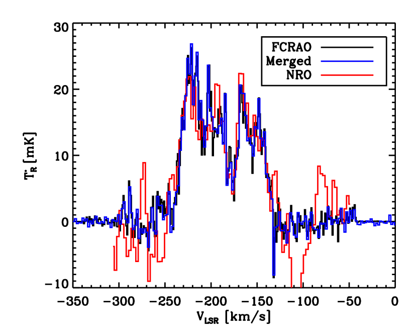
Figure 3.— Comparisons of the merged BIMA+FCRAO map with the NRO observations. (left) This panel compares the individual data values over the shared region between the two maps on an element-by-element basis showing reasonably good agreement within the uncertainties of the map. (right) This panel compares the average spectrum that would be derived for each data cube using a Gaussian beam with FWHM of $7^{\prime}$ (1.7 kpc) centered on the central position of the galaxy. The three spectra are for the merged BIMA+FCRAO data cube (blue), the FCRAO data set alone (black), and the NRO data (red).

Because the two data sets agree well over their common area, a final map of the central region of M33 requires simply averaging the two data cubes. The average was weighted by the inverse square of the noise estimate determined for each pixel in the data cube where the Chauvenet criterion (Taylor, 1997) was applied iteratively to remove high-significance outliers (see EPRB for details). The final data cube has a typical rms noise temperature of 60 mK and a resolution of 20^′′ $\times$ 2.6 km s^-1, corresponding to a projected resolution of 81 pc. At this angular resolution, the noise level of of the BIMA+FCRAO map is 100 mK, so combining the data yields a 40% improvement in the sensitivity. The NRO+FCRAO+BIMA map is shown in Figure 4; it will be referred to here as “the combined map.” Because of variable integration time and atmospheric conditions, the noise varies spatially across the map. Figure 5 shows the 1$\sigma$ rms noise level as a function of position for the final data cube. Table 2 compares the properties of the various maps.

Table 2 Map Properties

	FCRAO	BIMA+FCRAO	BIMA+FCRAO+NRO
	single dish	“merged”	“combined”
Resolution	$45^{\prime\prime}\times 1.0\mbox{ km s}^{-1}$	$13^{\prime\prime}\times 2.03~{}\mbox{km s}^{-1}$	$20^{\prime\prime}\times 2.6~{}\mbox{km s}^{-1}$
$V_{LSR}$ Coverage (km s-1)	$[-340,0]$	$[-340,0]$	$[-300,-49]$
Maximum $R_{gal}$ (kpc)	5.5	5.5	2.0
Mass Sensitivity ($M_{\odot}$)	$7.6\times 10^{4}$	$5\times 10^{4}$	$3.5\times 10^{4}$
Column Density Sensitivity(cm-2)	$8.2\times 10^{19}$	$7.5\times 10^{20}$	$2.2\times 10^{20}$
Central Flux (K km s-1)	$1.48\pm 0.02$	$1.47\pm 0.02$	$1.50\pm 0.01$

Figure 4.— Integrated intensity of CO emission in the central region of M33 from the combined NRO+BIMA+FCRAO data cube. At each position, the data have been integrated over a 20 channel (52 km s^-1) wide window centered on the line-of-sight projection of the rotation velocity at that position as derived from the rotation curve of Corbelli (2003), and the result is shown in negative grey scale. The noise varies across the map because of variable integration time and weather, and contours show the statistical significance based on local estimates of the noise level. Contour levels are $-4,-2$ (dotted),2,4…14 times the local rms. The center of the galaxy is indicated with a cross and is itself devoid of CO.

Figure 5.— Map of the 1$\sigma$ rms noise in the combined NRO+BIMA+FCRAO data cube. The noise varies because of differences in integration time across the map and changing atmospheric conditions during the observing. Dark areas indicate higher noise as shown by the scale bar on the right. Contours are drawn at noise levels of 60, 80, and 100 mK

4. Revisiting the Giant Molecular Clouds of M33

EPRB presented the first complete catalog of GMCs in M33 based on the BIMA survey data alone. The $13^{\prime\prime}$ (50 pc) resolution of the interferometer data is ideal for identifying individual GMCs though insufficient for measuring cloud sizes. The combination of the FCRAO and BIMA maps is even better for identifying GMCs because the data are not subject to many of the pathologies associated with interferometer-only data such as spatial filtering and non-linear flux recovery. In addition, the sensitivity of the merged map is marginally increased over the BIMA data alone because FCRAO and BIMA sample some of the same spatial frequencies. As shown in Figure 4, the molecular gas is distributed in many complexes with low surface brightness filaments connecting the complexes, which are also connected in velocity space. The bright CO complex in the north of the map contains the most massive molecular cloud in the galaxy (Cloud 1 of EPRB).

We have generated a new catalog of GMCs in M33 from the merged data set. The combined map is less suitable for the identification of GMCs since the coarser spatial and velocity resolution match GMCs poorly resulting in a higher completeness limit in the resulting catalog. The merged catalog is restricted to the region of overlap between the BIMA and FCRAO maps where all spatial information is recovered. The catalog was generated using a contouring method, as used by EPRB. The first step was to identify all regions in the data set with larger than a 2.7$\sigma_{rms}$ detection in two adjacent, independent channels. For each such detection, all pixels with significance larger than 2$\sigma_{rms}$ and connected to the 2.7$\sigma_{rms}$ “core” became part of the cloud candidate. For each candidate, we calculated the probability ($P$) of drawing the most significant spectrum from a random distribution of noise (see Appendix A of EPRB). We then multiplied by the number of independent measurements in the catalog region ($N\approx 2\times 10^{6}$) and considered $-\ln(NP)$ as the statistic of merit. The final catalog contains all candidates with $-\ln(NP)>8.0$ and with CO velocity centroids within 20 km s^-1 of the H I velocity centroid (Deul & van der Hulst, 1987) at that location. The selection criteria differ from those of EPRB, who included high significance detections across the entire bandpass and found four clouds at large velocity separation from the atomic gas. Subsequent observations of those apparent clouds showed that they are not real CO emitters but rather could be attributed to malfunctions in the BIMA correlator (Rosolowsky, Blitz & Engargiola, unpublished). We have selected a 20 km s^-1 separation from the H I velocity since this velocity range contains 90% of the CO flux (Figure 6) while containing no spurious sources.

Figure 6.— Cumulative distribution function (CDF) of CO emission found within a given velocity separation of the H I centroid, averaged over the entire CO map. Since 90% of the CO emission is found within 20 km s^-1 (dotted line), we limit our search for GMCs over this range.

Table 4 gives the new cloud catalog wherein objects are named “M33GMC.” Clouds are listed in order of increasing galactocentric radius. The cloud masses are based on a CO-to-H₂ conversion factor of $2\times 10^{20}\mbox{ cm}^{-2}(\mbox{K km s}^{-1})^{-1}$ and the previously-quoted distance of 840 kpc to M33 (Freedman et al., 2001). The conversion factor is appropriate for the GMCs in M33 and does not appear to vary significantly over the inner 4 kpc of the galaxy (Rosolowsky et al., 2003). The method for calculating mass differs from that of EPRB; masses here are based on the method of Rosolowsky & Leroy (2006). This method attempts to account for the amount of emission not included above the 2$\sigma_{rms}$ cutoff in the data cube by extrapolating the emission profile to the 0 K km s^-1 intensity contour. Accounting for this emission roughly doubles the derived cloud masses. Cloud major and minor axes and orientations are also given in Table 4; however, the sizes are not corrected for beam convolution and are thus upper limits. Deconvolution of the cloud sizes is unstable for large beam sizes (50 pc) and low signal-to-noise values (Rosolowsky & Leroy, 2006).

Table 3Catalog of GMC Properties

M33GMC	Position	$V_{\mathrm{GMC}}$	$V_{\mathrm{HI}}$	$R_{gal}$	$V_{\mathrm{GMC}}-V_{\mathrm{HI}}$	$-\ln(NP)$	Mass	$\sigma_{v}$	Size	Arm
	$(\alpha_{2000},\delta_{2000})$	(km s-1)	(km s-1)	(kpc)	(km s-1)		($10^{5}~{}M_{\odot}$)	(km s-1)	(pc$\times$pc)	Classification
1	01:33:52.4 +30:39:18	$-169.0$	$-169.0$	0.18	$0.0$	62.5	$3.1\pm 0.9$	$3.5\pm 0.9$	$82\times 62~{}(122^{\circ})$	Arm
2	01:33:49.5 +30:40:03	$-191.8$	$-185.3$	0.18	$-6.6$	42.9	$2.1\pm 0.5$	$4.5\pm 1.9$	$68\times 54~{}(12^{\circ})$	Arm
3	01:33:48.1 +30:39:31	$-168.4$	$-169.1$	0.21	$0.7$	15.1	$2.5\pm 2.1$	$2.6\pm 2.9$	$80\times 62~{}(105^{\circ})$	Arm
4	01:33:48.3 +30:38:53	$-158.0$	$-159.7$	0.23	$1.7$	32.3	$1.0\pm 0.5$	$2.3\pm 0.8$	$62\times 53~{}(85^{\circ})$	Arm
5	01:33:52.4 +30:40:32	$-209.9$	$-201.4$	0.24	$-8.4$	34.0	$1.7\pm 1.1$	$2.7\pm 1.2$	$67\times 58~{}(159^{\circ})$	Arm
6	01:33:49.6 +30:41:08	$-193.6$	$-199.5$	0.46	$5.9$	9.3	$1.6\pm 1.5$	$2.4\pm 2.0$	$82\times 60~{}(36^{\circ})$	Arm
7	01:33:56.8 +30:40:08	$-192.6$	$-195.0$	0.46	$2.4$	63.9	$3.5\pm 1.0$	$3.0\pm 0.8$	$115\times 63~{}(105^{\circ})$	Arm
8	01:33:44.6 +30:38:54	$-163.7$	$-161.0$	0.47	$-2.7$	12.3	$1.4\pm 1.0$	$3.1\pm 3.6$	$68\times 58~{}(103^{\circ})$	Arm
9	01:33:51.2 +30:41:29	$-220.3$	$-215.4$	0.50	$-4.9$	14.2	$2.5\pm 1.3$	$3.6\pm 1.8$	$98\times 50~{}(35^{\circ})$	Interarm
10	01:33:53.5 +30:41:41	$-224.9$	$-219.8$	0.53	$-5.1$	34.8	$1.7\pm 0.7$	$2.7\pm 1.1$	$70\times 53~{}(34^{\circ})$	Interarm
11	01:33:57.0 +30:41:08	$-213.4$	$-211.1$	0.54	$-2.2$	20.0	$1.4\pm 1.2$	$2.3\pm 0.9$	$68\times 60~{}(29^{\circ})$	Interarm
12	01:33:55.5 +30:41:37	$-221.8$	$-216.4$	0.55	$-5.4$	51.0	$4.8\pm 1.1$	$6.5\pm 1.7$	$107\times 82~{}(155^{\circ})$	Interarm
13	01:33:49.9 +30:37:27	$-149.5$	$-149.8$	0.57	$0.1$	12.4	$1.1\pm 1.4$	$4.9\pm 3.2$	$60\times 48~{}(90^{\circ})$	Interarm
14	01:33:47.9 +30:41:29	$-203.5$	$-200.6$	0.63	$-2.9$	32.1	$0.9\pm 0.5$	$1.6\pm 1.4$	$62\times 57~{}(70^{\circ})$	Arm
15	01:33:52.5 +30:42:15	$-214.0$	$-216.2$	0.68	$2.2$	21.7	$2.6\pm 1.6$	$3.7\pm 2.6$	$91\times 52~{}(172^{\circ})$	Interarm
16	01:33:43.1 +30:37:31	$-139.5$	$-142.8$	0.69	$3.2$	10.1	$0.4\pm 0.3$	$1.8\pm 2.5$	$60\times 49~{}(95^{\circ})$	Interarm
17	01:33:54.8 +30:37:43	$-167.7$	$-164.9$	0.69	$-2.8$	88.9	$2.2\pm 0.4$	$3.0\pm 1.0$	$63\times 57~{}(89^{\circ})$	Arm
18	01:33:59.9 +30:40:45	$-209.8$	$-207.3$	0.70	$-2.4$	204.3	$7.7\pm 0.9$	$4.5\pm 0.6$	$93\times 68~{}(107^{\circ})$	Interarm
19	01:33:52.9 +30:37:17	$-152.7$	$-154.0$	0.71	$1.3$	31.5	$4.7\pm 1.4$	$4.1\pm 1.3$	$165\times 68~{}(1^{\circ})$	Interarm
20	01:33:45.3 +30:36:52	$-144.2$	$-139.9$	0.73	$-4.3$	30.6	$1.9\pm 1.7$	$2.4\pm 1.5$	$66\times 59~{}(87^{\circ})$	Interarm
21	01:33:59.7 +30:41:32	$-221.5$	$-217.3$	0.74	$-4.2$	64.2	$4.5\pm 1.1$	$4.9\pm 1.2$	$82\times 64~{}(105^{\circ})$	Interarm
22	01:33:41.0 +30:39:14	$-166.2$	$-165.6$	0.77	$-0.6$	192.9	$6.0\pm 0.7$	$4.0\pm 0.9$	$75\times 66~{}(128^{\circ})$	Arm
23	01:33:57.8 +30:42:21	$-233.7$	$-229.9$	0.77	$-3.8$	14.3	$1.7\pm 1.0$	$3.2\pm 1.6$	$81\times 59~{}(165^{\circ})$	Interarm
24	01:33:43.5 +30:41:09	$-195.0$	$-195.7$	0.83	$0.7$	37.2	$2.2\pm 1.0$	$3.9\pm 1.3$	$73\times 52~{}(135^{\circ})$	Arm
25	01:33:44.3 +30:41:39	$-198.8$	$-198.8$	0.88	$-0.1$	15.9	$1.7\pm 1.4$	$4.1\pm 2.2$	$80\times 54~{}(76^{\circ})$	Arm
26	01:33:55.8 +30:43:02	$-227.3$	$-226.6$	0.88	$-0.7$	36.5	$6.3\pm 1.6$	$3.3\pm 1.2$	$137\times 72~{}(7^{\circ})$	Interarm
27	01:33:39.1 +30:38:00	$-149.4$	$-148.8$	0.91	$-0.7$	17.5	$1.3\pm 1.2$	$3.0\pm 2.2$	$73\times 50~{}(93^{\circ})$	Arm
28	01:33:44.9 +30:36:01	$-138.7$	$-138.5$	0.93	$-0.2$	61.6	$3.6\pm 1.2$	$4.0\pm 0.9$	$70\times 69~{}(49^{\circ})$	Interarm
29	01:34:02.3 +30:39:12	$-201.1$	$-195.4$	0.98	$-5.6$	38.3	$4.2\pm 1.3$	$4.1\pm 2.5$	$86\times 67~{}(85^{\circ})$	Arm
30	01:33:57.2 +30:36:41	$-166.7$	$-161.9$	1.08	$-4.9$	36.3	$1.1\pm 0.8$	$1.7\pm 0.7$	$65\times 61~{}(130^{\circ})$	Arm
31	01:34:02.8 +30:38:38	$-185.8$	$-186.4$	1.09	$0.6$	33.6	$5.9\pm 2.0$	$6.6\pm 2.8$	$173\times 62~{}(83^{\circ})$	Arm
32	01:33:42.1 +30:35:29	$-128.0$	$-129.7$	1.11	$1.5$	12.1	$0.6\pm 0.5$	$2.4\pm 2.3$	$56\times 51~{}(179^{\circ})$	Interarm
33	01:33:41.3 +30:41:47	$-205.6$	$-196.1$	1.11	$-9.5$	16.6	$2.5\pm 0.9$	$3.1\pm 1.2$	$79\times 60~{}(56^{\circ})$	Arm
34	01:33:36.9 +30:39:30	$-167.7$	$-163.6$	1.13	$-4.1$	43.1	$6.4\pm 1.5$	$3.7\pm 0.7$	$138\times 63~{}(88^{\circ})$	Arm
35	01:33:41.6 +30:35:14	$-127.2$	$-130.5$	1.17	$3.2$	8.1	$2.0\pm 2.5$	$5.9\pm 5.0$	$64\times 56~{}(136^{\circ})$	Interarm
36	01:34:01.3 +30:43:55	$-229.2$	$-228.3$	1.20	$-0.9$	44.5	$3.0\pm 0.8$	$2.9\pm 1.0$	$69\times 64~{}(60^{\circ})$	Interarm
37	01:33:35.7 +30:36:25	$-134.0$	$-132.8$	1.25	$-1.3$	54.4	$5.0\pm 1.1$	$2.7\pm 0.8$	$133\times 72~{}(112^{\circ})$	Interarm
38	01:33:34.8 +30:37:02	$-136.0$	$-137.7$	1.26	$1.6$	18.9	$1.5\pm 0.6$	$2.3\pm 0.6$	$69\times 59~{}(22^{\circ})$	Interarm
39	01:34:07.2 +30:41:41	$-217.7$	$-215.2$	1.27	$-2.5$	8.9	$2.0\pm 1.2$	$2.7\pm 1.4$	$75\times 54~{}(73^{\circ})$	Interarm
40	01:34:06.8 +30:39:28	$-202.5$	$-200.4$	1.32	$-2.1$	38.0	$1.3\pm 0.6$	$4.1\pm 1.8$	$62\times 54~{}(46^{\circ})$	Interarm
41	01:33:59.2 +30:36:08	$-153.3$	$-150.7$	1.33	$-2.6$	85.3	$2.8\pm 0.6$	$3.8\pm 1.1$	$101\times 57~{}(141^{\circ})$	Arm
42	01:34:01.7 +30:36:43	$-153.7$	$-154.7$	1.37	$1.0$	40.2	$3.1\pm 1.1$	$2.6\pm 0.9$	$79\times 67~{}(21^{\circ})$	Arm
43	01:33:32.1 +30:36:59	$-144.7$	$-141.4$	1.45	$-3.3$	14.5	$0.3\pm 0.3$	$1.6\pm 1.1$	$49\times 48~{}(142^{\circ})$	Interarm
44	01:33:31.9 +30:37:58	$-152.5$	$-153.0$	1.46	$0.4$	9.6	$1.4\pm 0.9$	$3.3\pm 1.4$	$75\times 54~{}(101^{\circ})$	Interarm
45	01:33:48.4 +30:44:44	$-227.4$	$-224.7$	1.46	$-2.7$	8.2	$2.1\pm 1.3$	$3.3\pm 1.8$	$82\times 64~{}(131^{\circ})$	Arm
46	01:34:08.8 +30:39:11	$-194.1$	$-193.2$	1.51	$-0.9$	119.5	$3.4\pm 0.7$	$3.0\pm 0.8$	$75\times 61~{}(85^{\circ})$	Interarm
47	01:33:50.4 +30:33:59	$-134.0$	$-129.9$	1.52	$-4.2$	30.5	$4.1\pm 0.9$	$3.6\pm 1.1$	$111\times 59~{}(54^{\circ})$	Arm
48	01:34:06.3 +30:37:41	$-163.5$	$-164.7$	1.52	$1.2$	51.8	$2.9\pm 0.7$	$3.5\pm 1.0$	$83\times 62~{}(79^{\circ})$	Arm
49	01:33:33.5 +30:41:22	$-185.6$	$-180.3$	1.63	$-5.4$	40.9	$2.5\pm 0.7$	$2.6\pm 1.1$	$82\times 57~{}(37^{\circ})$	Interarm
50	01:33:42.8 +30:33:10	$-119.3$	$-119.6$	1.65	$0.4$	49.9	$2.7\pm 1.6$	$2.8\pm 1.1$	$82\times 68~{}(6^{\circ})$	Arm
51	01:34:11.6 +30:43:15	$-220.0$	$-219.7$	1.66	$-0.3$	29.9	$2.3\pm 0.8$	$2.8\pm 1.2$	$77\times 62~{}(70^{\circ})$	Interarm
52	01:33:37.4 +30:43:11	$-201.0$	$-197.2$	1.68	$-3.8$	17.6	$0.9\pm 0.6$	$2.3\pm 1.1$	$59\times 53~{}(164^{\circ})$	Arm
53	01:34:04.0 +30:35:57	$-146.7$	$-146.7$	1.69	$-0.1$	14.4	$0.7\pm 0.5$	$1.6\pm 1.3$	$64\times 58~{}(87^{\circ})$	Arm
54	01:34:01.1 +30:46:09	$-238.6$	$-237.8$	1.69	$-0.7$	29.0	$1.5\pm 1.2$	$3.8\pm 2.3$	$76\times 55~{}(30^{\circ})$	Arm
55	01:34:08.6 +30:37:40	$-156.7$	$-168.8$	1.70	$12.2$	9.7	$0.7\pm 1.0$	$2.3\pm 1.9$	$64\times 53~{}(96^{\circ})$	Arm
56	01:33:59.9 +30:34:49	$-144.5$	$-140.5$	1.70	$-3.9$	43.3	$2.4\pm 1.1$	$3.5\pm 1.6$	$79\times 61~{}(113^{\circ})$	Arm
57	01:34:12.9 +30:42:00	$-209.8$	$-209.5$	1.70	$-0.2$	24.0	$1.8\pm 1.0$	$2.7\pm 1.6$	$86\times 52~{}(42^{\circ})$	Interarm
58	01:33:46.7 +30:45:29	$-232.2$	$-227.6$	1.73	$-4.5$	8.2	$1.2\pm 0.9$	$2.3\pm 1.8$	$66\times 50~{}(46^{\circ})$	Arm
59	01:34:10.8 +30:44:53	$-234.6$	$-236.0$	1.78	$1.4$	18.9	$2.7\pm 1.5$	$3.2\pm 2.5$	$74\times 66~{}(108^{\circ})$	Interarm
60	01:33:52.4 +30:33:10	$-127.6$	$-125.0$	1.79	$-2.5$	14.3	$1.9\pm 1.4$	$3.2\pm 1.4$	$73\times 59~{}(79^{\circ})$	Arm
61	01:33:46.9 +30:32:41	$-117.6$	$-114.3$	1.80	$-3.3$	73.4	$3.4\pm 1.2$	$4.1\pm 1.4$	$79\times 63~{}(29^{\circ})$	Arm
62	01:34:02.6 +30:46:32	$-245.6$	$-242.2$	1.80	$-3.4$	34.7	$1.9\pm 0.6$	$3.2\pm 1.2$	$74\times 56~{}(51^{\circ})$	Arm
63	01:33:52.5 +30:46:28	$-240.2$	$-238.1$	1.82	$-2.1$	17.5	$1.4\pm 1.3$	$3.0\pm 3.2$	$69\times 52~{}(173^{\circ})$	Arm
64	01:34:04.3 +30:46:33	$-248.8$	$-244.2$	1.84	$-4.6$	11.8	$3.0\pm 2.0$	$2.5\pm 2.8$	$72\times 63~{}(121^{\circ})$	Arm
65	01:33:29.0 +30:40:23	$-179.6$	$-177.0$	1.85	$-2.6$	21.3	$1.3\pm 0.9$	$4.2\pm 2.6$	$69\times 55~{}(95^{\circ})$	Interarm
66	01:34:13.3 +30:39:06	$-196.2$	$-196.5$	1.89	$0.3$	15.5	$1.1\pm 0.9$	$2.9\pm 2.4$	$75\times 48~{}(141^{\circ})$	Interarm
67	01:33:38.5 +30:32:20	$-123.6$	$-119.4$	1.89	$-4.2$	13.9	$0.9\pm 1.4$	$2.8\pm 2.0$	$66\times 50~{}(65^{\circ})$	Arm
68	01:33:44.2 +30:32:05	$-106.3$	$-111.9$	1.93	$5.6$	11.7	$0.5\pm 0.7$	$1.7\pm 2.4$	$62\times 53~{}(179^{\circ})$	Arm
69	01:34:10.8 +30:37:11	$-168.9$	$-169.0$	1.95	$0.1$	32.8	$4.1\pm 1.4$	$4.4\pm 1.7$	$78\times 61~{}(59^{\circ})$	Interarm
70	01:33:37.9 +30:44:45	$-211.0$	$-210.3$	2.00	$-0.7$	34.2	$3.7\pm 1.8$	$5.3\pm 1.6$	$79\times 59~{}(128^{\circ})$	Interarm
71	01:33:37.0 +30:31:58	$-121.5$	$-116.2$	2.01	$-5.3$	54.0	$0.9\pm 0.6$	$1.8\pm 0.7$	$65\times 58~{}(70^{\circ})$	Arm
72	01:33:32.1 +30:32:29	$-136.7$	$-126.5$	2.03	$-10.2$	16.9	$0.4\pm 0.3$	$2.0\pm 1.3$	$56\times 47~{}(179^{\circ})$	Arm
73	01:33:33.4 +30:32:14	$-130.4$	$-122.3$	2.03	$-8.1$	25.1	$1.0\pm 0.8$	$2.4\pm 1.5$	$71\times 52~{}(107^{\circ})$	Arm
74	01:34:12.4 +30:37:16	$-189.0$	$-179.9$	2.06	$-9.1$	44.3	$1.8\pm 1.3$	$4.1\pm 1.9$	$66\times 58~{}(115^{\circ})$	Interarm
75	01:33:33.2 +30:31:56	$-110.3$	$-116.9$	2.10	$6.5$	30.5	$0.8\pm 0.4$	$1.5\pm 0.6$	$62\times 57~{}(61^{\circ})$	Arm
76	01:34:10.7 +30:36:15	$-159.2$	$-164.3$	2.11	$5.0$	128.2	$3.5\pm 0.5$	$1.7\pm 0.7$	$90\times 64~{}(168^{\circ})$	Interarm
77	01:34:16.6 +30:39:17	$-189.5$	$-191.1$	2.13	$1.6$	59.6	$3.7\pm 0.9$	$2.6\pm 1.3$	$85\times 67~{}(47^{\circ})$	Interarm
78	01:33:30.3 +30:32:16	$-139.9$	$-125.1$	2.14	$-14.8$	17.4	$1.7\pm 2.7$	$2.4\pm 2.3$	$126\times 59~{}(73^{\circ})$	Arm
79	01:33:23.9 +30:39:09	$-158.9$	$-160.8$	2.15	$2.0$	14.5	$1.3\pm 1.0$	$4.0\pm 2.3$	$65\times 50~{}(133^{\circ})$	Interarm
80	01:33:40.7 +30:46:04	$-218.6$	$-217.6$	2.17	$-0.9$	88.3	$8.2\pm 1.3$	$5.3\pm 1.0$	$145\times 71~{}(12^{\circ})$	Interarm
81	01:34:06.6 +30:47:52	$-256.4$	$-254.2$	2.18	$-2.3$	106.6	$6.2\pm 0.7$	$3.5\pm 0.8$	$91\times 68~{}(124^{\circ})$	Arm
82	01:33:29.7 +30:31:56	$-132.8$	$-122.9$	2.22	$-10.0$	49.4	$3.8\pm 1.4$	$4.7\pm 1.8$	$97\times 71~{}(126^{\circ})$	Arm
83	01:34:03.7 +30:48:16	$-252.7$	$-250.0$	2.23	$-2.7$	24.8	$0.6\pm 0.5$	$1.7\pm 0.8$	$57\times 53~{}(80^{\circ})$	Arm
84	01:34:15.3 +30:46:27	$-247.6$	$-240.1$	2.23	$-7.5$	8.4	$1.0\pm 1.3$	$2.5\pm 1.0$	$70\times 54~{}(50^{\circ})$	Interarm
85	01:34:15.8 +30:46:34	$-236.3$	$-240.1$	2.27	$3.8$	9.7	$0.9\pm 0.7$	$3.1\pm 2.8$	$68\times 50~{}(60^{\circ})$	Interarm
86	01:33:59.1 +30:48:59	$-248.1$	$-245.3$	2.40	$-2.8$	264.1	$12.8\pm 0.8$	$5.0\pm 0.7$	$178\times 82~{}(21^{\circ})$	Interarm
87	01:34:04.7 +30:49:00	$-250.2$	$-249.4$	2.42	$-0.9$	17.5	$2.8\pm 1.6$	$3.2\pm 1.2$	$91\times 71~{}(73^{\circ})$	Interarm
88	01:34:08.4 +30:33:51	$-159.5$	$-155.9$	2.44	$-3.6$	31.6	$1.6\pm 0.9$	$2.6\pm 1.4$	$76\times 53~{}(37^{\circ})$	Interarm
89	01:34:11.7 +30:48:32	$-259.3$	$-248.0$	2.45	$-11.3$	34.6	$3.3\pm 1.2$	$4.4\pm 1.4$	$142\times 57~{}(137^{\circ})$	Arm
90	01:33:23.9 +30:32:00	$-122.4$	$-120.6$	2.46	$-1.8$	52.3	$4.0\pm 1.3$	$3.7\pm 1.0$	$87\times 70~{}(101^{\circ})$	Arm
91	01:34:09.2 +30:49:06	$-249.0$	$-247.5$	2.51	$-1.5$	301.1	$11.1\pm 0.8$	$5.0\pm 0.8$	$83\times 71~{}(61^{\circ})$	Interarm
92	01:33:46.5 +30:48:22	$-233.2$	$-234.5$	2.51	$1.3$	22.9	$1.1\pm 0.8$	$2.5\pm 1.2$	$63\times 53~{}(157^{\circ})$	Interarm
93	01:34:14.1 +30:48:29	$-252.8$	$-249.9$	2.52	$-2.9$	14.0	$0.6\pm 0.6$	$1.9\pm 2.2$	$57\times 57~{}(81^{\circ})$	Arm
94	01:34:22.0 +30:39:46	$-205.2$	$-204.0$	2.53	$-1.2$	8.5	$0.7\pm 0.6$	$4.3\pm 3.8$	$82\times 51~{}(119^{\circ})$	Interarm
95	01:33:42.1 +30:47:46	$-237.0$	$-233.6$	2.53	$-3.4$	37.5	$5.0\pm 1.2$	$3.4\pm 1.3$	$163\times 66~{}(59^{\circ})$	Interarm
96	01:33:21.3 +30:32:04	$-120.4$	$-123.4$	2.59	$2.9$	20.5	$1.9\pm 1.1$	$2.5\pm 1.1$	$71\times 61~{}(98^{\circ})$	Arm
97	01:34:14.6 +30:35:11	$-162.8$	$-166.8$	2.59	$4.0$	9.9	$0.6\pm 0.7$	$2.7\pm 4.0$	$63\times 47~{}(99^{\circ})$	Interarm
98	01:33:38.9 +30:47:23	$-225.1$	$-225.3$	2.59	$0.2$	10.2	$0.8\pm 1.0$	$3.0\pm 2.3$	$60\times 57~{}(98^{\circ})$	Interarm
99	01:34:13.8 +30:34:38	$-174.1$	$-171.3$	2.65	$-2.8$	43.3	$4.4\pm 1.4$	$4.5\pm 1.2$	$89\times 72~{}(162^{\circ})$	Interarm
100	01:34:08.1 +30:32:50	$-145.3$	$-149.5$	2.66	$4.2$	16.0	$2.3\pm 1.5$	$2.6\pm 1.6$	$110\times 59~{}(29^{\circ})$	Interarm
101	01:34:17.7 +30:48:36	$-248.5$	$-245.5$	2.68	$-3.0$	24.8	$1.2\pm 1.0$	$2.2\pm 1.7$	$67\times 51~{}(66^{\circ})$	Arm
102	01:34:18.5 +30:48:23	$-245.1$	$-244.2$	2.68	$-0.9$	14.0	$1.2\pm 0.8$	$3.5\pm 1.8$	$64\times 49~{}(29^{\circ})$	Arm
103	01:34:10.0 +30:49:53	$-261.1$	$-258.6$	2.70	$-2.4$	10.3	$1.8\pm 0.6$	$3.5\pm 1.9$	$97\times 54~{}(92^{\circ})$	Interarm
104	01:33:18.5 +30:40:56	$-178.8$	$-172.7$	2.77	$-6.1$	15.2	$1.1\pm 0.9$	$2.3\pm 1.6$	$67\times 63~{}(164^{\circ})$	Interarm
105	01:34:13.6 +30:33:44	$-156.6$	$-157.9$	2.82	$1.3$	158.2	$5.0\pm 0.7$	$4.0\pm 0.9$	$70\times 64~{}(30^{\circ})$	Interarm
106	01:34:19.2 +30:49:05	$-227.5$	$-246.1$	2.83	$18.6$	10.0	$0.7\pm 0.7$	$3.1\pm 2.2$	$58\times 50~{}(177^{\circ})$	Arm
107	01:33:18.5 +30:41:34	$-178.6$	$-175.5$	2.85	$-3.1$	31.7	$1.5\pm 0.8$	$3.0\pm 1.5$	$69\times 57~{}(171^{\circ})$	Interarm
108	01:33:39.3 +30:28:20	$-104.3$	$-104.9$	2.88	$0.6$	8.9	$0.8\pm 1.0$	$2.0\pm 1.4$	$79\times 49~{}(59^{\circ})$	Interarm
109	01:34:22.6 +30:48:45	$-249.5$	$-244.2$	2.93	$-5.3$	23.6	$5.5\pm 1.4$	$3.1\pm 1.2$	$138\times 68~{}(88^{\circ})$	Arm
110	01:34:10.0 +30:31:52	$-148.7$	$-148.5$	3.01	$-0.1$	10.9	$0.6\pm 0.8$	$2.3\pm 1.5$	$72\times 47~{}(9^{\circ})$	Interarm
111	01:33:13.6 +30:39:28	$-160.6$	$-160.0$	3.02	$-0.7$	38.0	$1.3\pm 0.7$	$2.8\pm 2.2$	$59\times 59~{}(171^{\circ})$	Interarm
112	01:33:54.0 +30:51:04	$-247.5$	$-255.8$	3.03	$8.4$	10.6	$1.4\pm 1.8$	$2.9\pm 3.8$	$61\times 53~{}(49^{\circ})$	Interarm
113	01:33:32.0 +30:47:37	$-214.4$	$-214.0$	3.04	$-0.4$	25.5	$0.9\pm 0.6$	$3.5\pm 2.2$	$52\times 51~{}(144^{\circ})$	Interarm
114	01:33:15.3 +30:41:14	$-165.0$	$-166.7$	3.07	$1.7$	24.2	$1.3\pm 0.5$	$3.1\pm 1.7$	$74\times 54~{}(62^{\circ})$	Interarm
115	01:33:18.4 +30:29:38	$-106.5$	$-102.4$	3.10	$-4.0$	11.9	$0.5\pm 0.7$	$1.9\pm 1.6$	$68\times 56~{}(92^{\circ})$	Interarm
116	01:34:17.7 +30:33:41	$-159.3$	$-157.3$	3.11	$-2.0$	21.2	$2.2\pm 2.4$	$3.6\pm 2.0$	$106\times 67~{}(132^{\circ})$	Interarm
117	01:33:12.0 +30:39:32	$-162.7$	$-159.8$	3.15	$-2.9$	21.6	$1.3\pm 0.9$	$3.8\pm 1.5$	$84\times 48~{}(27^{\circ})$	Interarm
118	01:34:18.7 +30:33:48	$-166.7$	$-158.8$	3.17	$-7.9$	10.0	$0.6\pm 1.1$	$2.3\pm 2.1$	$61\times 54~{}(54^{\circ})$	Interarm
119	01:34:21.7 +30:34:55	$-187.6$	$-179.0$	3.18	$-8.7$	12.7	$0.7\pm 0.7$	$3.6\pm 1.8$	$88\times 47~{}(90^{\circ})$	Interarm
120	01:34:27.4 +30:49:12	$-248.4$	$-245.0$	3.24	$-3.5$	21.6	$4.0\pm 1.1$	$3.7\pm 1.2$	$111\times 61~{}(51^{\circ})$	Interarm
121	01:34:16.7 +30:51:39	$-266.9$	$-264.3$	3.25	$-2.6$	10.3	$1.9\pm 1.1$	$3.1\pm 2.0$	$80\times 60~{}(25^{\circ})$	Interarm
122	01:34:31.7 +30:47:37	$-252.5$	$-246.2$	3.32	$-6.3$	16.1	$1.7\pm 1.2$	$2.5\pm 1.6$	$96\times 64~{}(61^{\circ})$	Arm
123	01:34:31.9 +30:47:42	$-243.2$	$-246.1$	3.34	$2.8$	11.3	$2.3\pm 1.2$	$3.1\pm 1.3$	$66\times 66~{}(12^{\circ})$	Arm
124	01:34:33.0 +30:46:47	$-243.0$	$-242.0$	3.35	$-1.1$	125.2	$10.0\pm 1.1$	$4.1\pm 0.8$	$117\times 87~{}(149^{\circ})$	Arm
125	01:34:15.9 +30:52:19	$-266.1$	$-262.0$	3.37	$-4.1$	11.8	$2.3\pm 1.4$	$3.3\pm 1.6$	$87\times 55~{}(79^{\circ})$	Interarm
126	01:34:34.5 +30:46:19	$-221.8$	$-235.1$	3.42	$13.2$	96.0	$3.5\pm 0.7$	$3.9\pm 1.0$	$78\times 60~{}(27^{\circ})$	Arm
127	01:33:05.7 +30:35:08	$-144.4$	$-144.0$	3.47	$-0.4$	31.4	$0.9\pm 0.6$	$2.0\pm 1.1$	$62\times 61~{}(86^{\circ})$	Interarm
128	01:33:44.0 +30:51:47	$-241.5$	$-236.9$	3.52	$-4.6$	16.6	$1.9\pm 1.8$	$4.6\pm 5.2$	$61\times 54~{}(56^{\circ})$	Interarm
129	01:33:39.9 +30:51:22	$-251.0$	$-233.2$	3.58	$-17.8$	8.4	$0.6\pm 0.5$	$2.7\pm 1.8$	$57\times 48~{}(172^{\circ})$	Interarm
130	01:34:14.4 +30:30:26	$-151.8$	$-150.7$	3.61	$-1.2$	16.3	$0.6\pm 0.5$	$2.3\pm 1.3$	$82\times 57~{}(9^{\circ})$	Interarm
131	01:34:22.8 +30:32:41	$-166.0$	$-158.1$	3.68	$-7.9$	33.0	$2.4\pm 1.0$	$2.7\pm 1.1$	$91\times 63~{}(92^{\circ})$	Interarm
132	01:33:23.6 +30:25:40	$-112.2$	$-109.8$	3.70	$-2.5$	78.9	$4.4\pm 0.7$	$3.1\pm 0.8$	$82\times 69~{}(121^{\circ})$	Interarm
133	01:34:39.0 +30:43:57	$-220.1$	$-217.6$	3.71	$-2.5$	11.8	$0.5\pm 0.4$	$1.3\pm 1.4$	$61\times 54~{}(63^{\circ})$	Arm
134	01:33:13.0 +30:27:22	$-115.4$	$-119.7$	3.71	$4.2$	19.7	$2.7\pm 1.7$	$3.0\pm 1.1$	$116\times 60~{}(2^{\circ})$	Interarm
135	01:33:10.6 +30:27:43	$-122.5$	$-117.0$	3.76	$-5.6$	28.5	$2.2\pm 0.8$	$2.8\pm 1.1$	$82\times 54~{}(39^{\circ})$	Interarm
136	01:34:38.3 +30:40:30	$-199.9$	$-202.6$	3.80	$2.7$	108.1	$10.7\pm 1.1$	$8.4\pm 1.5$	$239\times 106~{}(52^{\circ})$	Arm
137	01:33:03.7 +30:39:56	$-164.4$	$-165.2$	3.87	$0.7$	16.9	$0.8\pm 0.8$	$3.2\pm 1.4$	$55\times 51~{}(144^{\circ})$	Interarm
138	01:34:41.4 +30:47:10	$-236.3$	$-238.6$	3.95	$2.4$	12.4	$1.4\pm 0.9$	$2.8\pm 2.6$	$74\times 55~{}(112^{\circ})$	Interarm
139	01:34:04.1 +30:55:09	$-256.5$	$-256.6$	3.98	$0.0$	11.8	$1.9\pm 1.0$	$4.2\pm 2.6$	$75\times 53~{}(37^{\circ})$	Interarm
140	01:34:33.4 +30:35:17	$-176.5$	$-172.7$	4.02	$-3.7$	24.0	$1.6\pm 0.9$	$2.1\pm 1.1$	$115\times 57~{}(132^{\circ})$	Interarm
141	01:34:36.0 +30:36:22	$-182.7$	$-179.8$	4.06	$-2.9$	8.1	$0.9\pm 1.1$	$5.3\pm 4.3$	$74\times 53~{}(146^{\circ})$	Interarm
142	01:34:29.7 +30:55:30	$-253.3$	$-262.9$	4.42	$9.6$	10.3	$1.6\pm 0.4$	$3.8\pm 1.3$	$62\times 60~{}(36^{\circ})$	Interarm
143	01:34:07.2 +30:57:52	$-266.8$	$-258.6$	4.68	$-8.1$	8.4	$1.3\pm 1.1$	$2.3\pm 2.9$	$96\times 56~{}(45^{\circ})$	Interarm
144	01:32:44.2 +30:35:12	$-144.0$	$-148.0$	5.17	$4.0$	10.3	$1.2\pm 0.6$	$4.0\pm 2.3$	$69\times 51~{}(55^{\circ})$	Interarm
145	01:33:16.9 +30:52:53	$-219.7$	$-216.6$	5.21	$-3.1$	9.2	$0.9\pm 0.4$	$3.6\pm 2.1$	$61\times 48~{}(50^{\circ})$	Interarm
146	01:32:42.1 +30:36:35	$-155.4$	$-153.8$	5.39	$-1.6$	8.5	$0.9\pm 0.5$	$2.1\pm 1.1$	$58\times 52~{}(166^{\circ})$	Interarm
147	01:32:42.2 +30:22:27	$-101.6$	$-101.4$	5.98	$-0.1$	12.4	$1.1\pm 0.6$	$2.5\pm 1.2$	$62\times 55~{}(92^{\circ})$	Interarm
148	01:33:10.5 +30:56:42	$-202.4$	$-214.4$	6.50	$12.0$	8.6	$1.0\pm 0.9$	$6.9\pm 3.5$	$59\times 49~{}(175^{\circ})$	Interarm
149	01:32:11.5 +30:30:18	$-134.2$	$-128.5$	7.65	$-5.7$	8.4	$0.9\pm 0.9$	$3.3\pm 2.5$	$58\times 51~{}(19^{\circ})$	Interarm

It is possible that the catalog method adopted in this study will blend together individual GMCs into a larger complex that, at higher resolution, would be identified as separate clouds. In their study of this problem, EPRB found many instances of cloud groups identified as distinct in the high-resolution work of Wilson & Scoville (1990) that were merged in the EPRB catalog. The same effects must be present in the current catalog and will affect studies of the mass distributions below §5. In general, appropriately decomposing a blend moves an individual cloud to multiple clouds of lower masses, steepening the mass distribution and reinforcing any truncations in the distribution (provided the mass of the original cloud was near the truncation mass). We proceed with this caveat in mind but make no effort to separate the catalog objects into smaller units. Decomposing blends is inaccurate at this physical resolution (50 pc; Rosolowsky & Leroy, 2006).

The new catalog contains 149 clouds to an estimated completeness limit of $1.3\times 10^{5}$ $M_{\sun}$. The limit is based on linearly scaling the completeness limit derived from EPRB’s detailed examination of the BIMA-only survey to the sensitivity limit in the BIMA+FCRAO data. The noise level of the merged map does not vary significantly in the region where molecular clouds are found, although it does increase in the outer regions of the galaxy. The original catalog of EPRB contained 144 clouds (omitting the spurious high-velocity outliers) with total mass $1.7\times 10^{7}$ $M_{\sun}$. Total mass of clouds in the new catalog would be $2.0\times 10^{7}$ $M_{\sun}$ using the same mass formula as EPRB. This increase in the mass estimate stems from inclusion of the low surface brightness emission that is not detected in the interferometer-only map. The larger increase in the catalog GMC mass, to $3.9\times 10^{7}$ $M_{\sun}$, comes from accounting for the flux below the 2$\sigma_{rms}$ limit. This total mass accounts for about 1/3 of all the mass implied by emission in the merged map, $1.2\times 10^{8}$ $M_{\sun}$. (This differs from the value reported by HCSY in part because we include helium and adopt a different distance and CO-to-H₂ conversion factor.) The remaining 2/3 of the emission is from sources that are of smaller mass than GMCs. This represents quite a contrast to the inner Milky Way, where the GMCs comprise 80% of the molecular mass (Williams & McKee, 1997).

The amount of CO emission from low mass clouds can be examined by averaging the data in annuli of galactocentric radius. Figure 7 compares the radial surface density profile for GMCs ($M>10^{5}~{}M_{\odot}$) and for all CO emission. Within 1 kpc of M33’s center, GMCs comprise $\lesssim$60% of the total molecular mass, and the fraction decreases rapidly with radius to $<$10% near $R_{gal}\approx 4.0$ kpc. Beyond that radius, GMCs vanish almost entirely with only a few, low-mass clouds beyond this radius although there is plenty of molecular gas. The dearth of GMCs beyond 4 kpc is real: the catalog completeness limit is only 10% higher in mass at $R_{gal}=5$ kpc than at $R_{gal}=0$. Thus there are significantly fewer GMCs per unit total molecular mass beyond $R_{gal}=4.1$ kpc than within that radius. The radius 4 kpc corresponds to the outer ends of the major spiral arms in M33 identified in N I and S I (Humphreys & Sandage, 1980). In addition, the neon abundance shows a sharp drop at this radius (Willner & Nelson-Patel, 2002). However, star formation as traced by H$\alpha$ continues out to $R_{gal}=6.7$ kpc (Kennicutt, 1989), and the disk is gravitationally unstable to that radius (Corbelli, 2003). Whatever the explanation for the changing conditions at $R_{gal}>4$ kpc, star formation in the outer part of M33 must occur in molecular clouds with $M\lesssim 1.3\times 10^{5}$ $M_{\sun}$. It is worth noting that this effect confounded the total mass estimate of EPRB who extrapolated the GMC mass to the total mass of the galaxy based on the fraction of emission in GMCs for the center of the galaxy.

Figure 7.— Radial surface density of molecular gas mass. The top panel shows the total mass surface density (upper curve) and the surface density of mass in GMCs ($M>10^{5}~{}M_{\odot}$ — lower curve). The bottom panel shows the ratio between these quantities. Error bars show the uncertainties in each 500 pc bin. At nearly all radii, GMCs comprise a minority of the total molecular gas mass, and the fraction declines from the galactic center. There appears to be a sharp cutoff in the distribution of GMCs at $R_{gal}\sim 4.0$ kpc, but the total molecular gas surface density profile continues beyond that radius.

The location of the low mass clouds in the inner region of M33 is shown directly in the combined map (Figure 8) with its 50% lower rms noise. The size of objects identified in the merged map is indicated with ellipses, representing the size and orientation of the objects as they would appear in the combined map after accounting for the differing resolutions and sensitivities. Emission beyond the boundaries of the identified GMCs arises from low mass clouds. This emission forms a filamentary structure, generally surrounding and linking the high mass GMCs. The GMCs themselves appear to define the compact peaks of the lower surface brightness structures. The low mass clouds are clearly correlated with the high mass GMCs, and we quantify this relationship by measuring the amount of flux found within a given separation from the edge of a catalog GMC. The results are shown in Figure 9 which plots the cumulative distribution of CO flux as a function of projected separation from the edge of the catalog GMCs shown in Figure 8. The curve rises from $\sim 30\%$ at zero separation (the amount of flux in GMCs) to over 90% at 100 pc separation. The dotted curve indicates the fraction of the area found within the same separation, which would be the curve that the flux distribution would follow if there were no spatial correlation between low mass and high mass clouds. The excess above the dotted curve shows the spatial correlation of the emission. There is no evidence for a galaxy-spanning, diffuse molecular gas component, confirming the conclusions of Rosolowsky et al. (2003).

Figure 8.— Map of the integrated intensity of CO emission in the central region of M33 in gray scale from the combined NRO+BIMA+FCRAO map. The gray scale runs linearly from 0 to 8 K km s^-1 and a contour is drawn at 1 K km s^-1. Positions of GMCs are indicated with red (blue) ellipses for clouds above (below) the $1.3\times 10^{5}~{}M_{\odot}$ completeness limit of the revised catalog from the BIMA+FCRAO map. The extent of the ellipses is determined by the size of the object in the merged map, extrapolated to the zero intensity contour and convolved to the resolution of the combined map. The border of the NRO observations is shown as a green line. Faint CO emission associated with low mass clouds is found around the high mass molecular clouds.

Figure 9.— Cumulative distribution of CO flux as a function of separation from the edges of the GMCs shown in Figure 8 using the combined BIMA+FCRAO+NRO map. The solid line represents the flux distribution and the dotted line shows the cumulative distribution of the survey area. The excess of the flux curve over the area curve shows the spatial correlation of the CO flux from low-mass clouds with the cataloged GMCs. Since the separation is measured from the edge of GMCs rather than the center, the curves begin with the 33% of the emission found in GMCs which are found in the 10% of the map area.

5. Variations in the GMC Mass Distribution

5.1. Radial Variation

The cloud size distribution varies with galactocentric radius in a surprising way. Fig. 7 shows the absence of GMCs beyond 4.1 kpc, but the most massive clouds ($M>8\times 10^{5}$ $M_{\sun}$) are also absent inside a radius of 2.1 kpc. Indeed all six clouds with $M>8\times 10^{5}$ $M_{\sun}$ are at $2.1\lesssim R_{gal}\lesssim 2.5$ kpc. Evidently something in the inner galaxy eliminates very large clouds, and something in the outer galaxy eliminates GMCs nearly altogether.

To examine the cloud distribution more quantitatively, we consider two regions divided at $R_{gal}=2.1$ kpc. This division yields approximately equal GMC mass in each region. Figure 10 shows the mass functions for the GMCs in these two regions. The mass distributions are significantly different. In the outer GMC region (the annulus $2.1<R_{gal}<4.1$ kpc), the GMC mass distribution follows a power law from high mass down to the completeness limit of the catalog. In the inner region, however, despite the existence of many more GMCs (about three times more per unit area), the mass distribution is truncated at the high end and may also fall slightly below a power law distribution at the low end. A two-sided KS test (Press et al., 1992) shows there is only a 0.8% probability that the two samples could be drawn from a single distribution while exhibiting such a large difference.

Figure 10.— Cumulative mass distribution of GMCs in the inner (blue, $R_{gal}<2.1$ kpc) and outer (black, $R_{gal}>2.1$ kpc) regions of M33. A power law cumulative mass distribution is shown for the outer galaxy (black dashed line), and truncated and non-truncated power law distributions are shown for the inner galaxy (blue dashed and red solid lines respectively). The vertical dotted line indicates the completeness limit for the survey.

The cumulative mass distribution functions can be characterized quantitatively by truncated power-law functions with the form:

$$N(M^{\prime}>M)=N_{0}\left[\left(\frac{M}{M_{0}}\right)^{\gamma+1}-1\right],$$ (1)

where $N_{0}$, $M_{0}$, and $\gamma$ are parameters, and the fit is restricted to clouds above the completeness limit of $1.3\times 10^{5}~{}M_{\odot}$. This functional form is adopted for comparison with the GMC population in the Milky Way. The parameter $\gamma$ is the index of the mass distribution. If $\gamma<-2$, most of the mass is found in low mass clouds, and if $\gamma>-2$, the high mass clouds dominate as is the case for the inner Milky Way. As long as $N_{0}$ is significantly larger than unity, the mass distribution has a truncation near $M=2^{1/(\gamma+1)}M_{0}$. In the inner Milky Way, the mass distribution is commonly expressed as a differential mass distribution. The differential mass distribution is well-characterized by a power-law with a truncation at large cloud masses ($M_{0}\sim 6\times 10^{6}~{}M_{\odot}$ Williams & McKee, 1997, and references therein):

$$\frac{dN}{dM}\propto\left(\frac{M}{M_{0}}\right)^{\gamma},~{}M<M_{0}.$$ (2)

A similar form of the distribution, albeit with different slopes, has been reported in the outer Milky Way (e.g. Heyer et al., 2001), the LMC (Fukui et al., 2001), M33 (EPRB), and other systems farther afield. Fitting the cumulative distribution instead of the differential one is a better way to describe the data because the cumulative function is not affected by biases introduced by binning, and it can account for uncertainties in the cloud masses (Rosolowsky, 2005). Table 4 gives the best-fit coefficients for the M33 data, and the resulting distributions are plotted Figure 10. As noted above, there is no significant truncation of the mass distribution for the outer galaxy clouds, and Table 4 reports coefficients for a simple power law fit. For comparison, Table 4 also includes the fit to the cumulative mass distribution of all the clouds in the catalog. Both the fits and Figure 10 indicate that the primary difference between the two distributions is the truncation in the upper end of the mass distribution of the inner galaxy clouds. No such truncation is apparent in the outer portion of the galaxy, and including one in the fit does not appreciably change the derived values or goodness of fit. In the mass range where the inner galaxy distribution fits a power law, $1.3<M/(10^{5}~{}M_{\odot})<5.0$, the two distributions are indistinguishable. While the inner galaxy has a larger fraction of its molecular gas in GMCs (Figure 7), the formation or survival of the highest-mass GMCs ($\gtrsim 7\times 10^{5}~{}M_{\odot}$) is suppressed. One possibility is that high mass clouds are sheared apart by galactic tides in this region; but this possibility is unlikely because clouds with masses of $10^{7}~{}M_{\odot}$ would be stable according to the criteria of Stark & Blitz (1978).

Table 4Parameters of Mass Distributions in M33

Objects	$\gamma$	$N_{0}$	$M_{0}/(10^{5}~{}M_{\odot})$
All Clouds	$-2.0\pm 0.2$	$11\pm 2$	$14\pm 7$
Radial Variation
Outer galaxy	$-2.1\pm 0.1$	$\cdots$	$34\pm 14$
Inner galaxy	$-1.8\pm 0.2$	$21\pm 11$	$7.4\pm 0.5$
Inner galaxy	$-2.4\pm 0.2$	$\cdots$	$23\pm 5$
North-South Variation
North	$-2.0\pm 0.2$	$5.4\pm 4.3$	$34\pm 12$
North	$-2.25\pm 0.15$	$\cdots$	$34\pm 11$
South	$-1.4\pm 0.2$	$41\pm 11$	$6.4\pm 0.5$
South	$-2.4\pm 0.3$	$\cdots$	$20\pm 16$
Arm-Interarm Variation
Arm	$-1.9\pm 0.2$	$5\pm 4$	$16\pm 5$
Interarm	$-2.2\pm 0.2$	$4\pm 4$	$13\pm 4$

The mass truncation and differences in the slope of the distribution may be effected by several aspects of the observations and the cataloging procedure, but none of the likely effects would produce a truncation where none is present. Wilson & Scoville (1990) have already reported a truncation in the mass distribution of GMCs, but it is difficult to assess their results as their survey is spatially incomplete and selected targets based on dust and CO priors. Since the merged data span the entire galaxy, spatial biases will not affect the mass distribution. The Wilson & Scoville (1990) data had significantly higher resolution and several of the clouds considered as separate in their study are not resolved into individual clouds here (or in EPRB, see their §3.5 and Figures 13 and 14). Blending will act to minimize the effects of truncation since separate small clouds will appear as a single cloud of higher mass, so the truncations are certainly present in the GMC mass distributions. The correction for emission found below the $2\sigma$ boundary of the clouds will also change the mass distribution slightly. Since flux loss primarily affects clouds near the completeness limit (since most of the emission in these clouds is below the identification contour), correcting for the effects of the flux loss will move these clouds to higher mass, thereby steepening the spectrum. Since this is a correction for an instrumental effect, making this correction likely improves estimates of the mass distribution. Finally, regardless of the precise nature of the systematic effects on the measured mass distributions, this reported measurement is differential between two regions cataloged with a uniform method. As such, the reported differences must reflect some underlying difference in the character of molecular gas in the two regions.

Similar variations in the GMC mass distribution as a function of position in a galaxy have not been directly quantified in previous work, but there is some evidence for such variations in the Milky Way. Rosolowsky (2005) argued for different mass distribution functions between the inner and outer Galaxy. This variation within the Milky Way is uncertain, however, because differences in cloud cataloging methods can produce apparent differences in the mass distribution while the underlying cloud populations are the same. In addition, large arm-interarm contrasts observed in many spiral galaxies suggest that the mass distribution of GMCs changes azimuthally (see also §5.3).

5.2. North-South Variation

The right-hand panel of Figure 3 implies that the approaching and receding sides of the galaxy have a significant flux asymmetry. The northern (approaching) portion of the galaxy has a total flux of $8200\mbox{ Jy km s}^{-1}$ whereas the southern (receding) half of the galaxy has a flux of $7800\mbox{ Jy km s}^{-1}$, a difference of $5\%$. The asymmetry is also seen in the H I (where the approaching half of the galaxy has 13% more flux than the receding) and the H$\alpha$ (5%) distributions (based on the images of Massey et al., 2006), making M33 slightly lopsided. Motivated by this flux asymmetry, we also consider the variation in the GMC mass distributions between the northern and southern halves of the galaxy. We define the southern (receding) portion of the galaxy as the portion of the disk with galactocentric azimuth within $90^{\circ}$ of the kinematic major axis and the northern region as the complement of the southern region. We fit truncated power-laws to the two distributions and report the derived parameters in Table 4. Like the variation between the inner and the outer galaxies, there is substantial difference between the northern and southern mass distribution, particularly at high masses. The southern portion of the galaxy lacks high mass clouds that are present in the northern portion of the galaxy. Both mass distributions have some evidence for truncation at the high masses, though the evidence is relatively weak for clouds in the northern portion of the galaxy. While it would be interesting to separate the variation in the mass distributions into 4 separate regions (inner vs. outer and northern vs. southern), we lack sufficient numbers of clouds for reliable fits. Since differences between the inner and outer regions of the galaxy are more pronounced, we focus our analysis on these difference, though with better data, the north-south asymmetry could be explored.

5.3. Arm-Interarm Variation

For galaxies with well defined spiral structure, the spiral arms contain nearly all of the molecular material in the galaxy (Vogel et al., 1999; Regan et al., 2001; Nieten et al., 2006). The Milky Way appears to be such a galaxy (e.g. Dame et al., 2001; Stark & Lee, 2006). Molecular gas in the interarm regions of spiral galaxies appears to have different properties than that found in the arms (Walsh et al., 2002; Tosaki et al., 2002; Stark & Lee, 2006) though Tosaki et al. (2003) suggest that the properties of individual GMCs may not vary significantly. While our observations lack the resolution to assess whether the GMC properties are substantially different in interarm regions of M33, we can investigate whether there is variation in the mass distributions of GMCs in and out of spiral arms. Unfortunately, the spiral arms in M33 are not nearly as well defined as they are in the Milky Way. Humphreys & Sandage (1980) identified ten spiral arms in the flocculent structure of M33 with two arms being dominant. Humphreys & Sandage attributed the two primary arms to spiral density waves. This conjecture was bolstered by observations in the near infrared, which revealed that the spiral structure of the old stellar population, and hence the stellar mass, was dominated by these two “grand design” spiral arms (Regan & Vogel, 1994). The remaining eight arms are mainly located in the outer galaxy. They were primarily defined by the presence of young stellar associations but also correlate well with narrow filaments of atomic gas (Deul & van der Hulst, 1987, EPRB). Humphreys & Sandage attributed these eight secondary arms to an unknown mechanism other than density waves.

For present purposes, we have defined the locations of the M33 spiral arms using a 3.6 $\mu$m image of the galaxy taken using the IRAC instrument of the Spitzer Space Telescope (Gehrz et al., 2005). A small correction was made for dust emission in the 3.6 µm image leaving emission primarily from the old stellar population. An azimuthally-symmetric exponential disk was fit to the result. The spiral arms become apparent as regions of positive surface brightness after subtracting the model disk. Detailed analysis will be presented elsewhere, but Figure 2 shows the spiral arm locations with respect to the CO emission.

Figure 11 compares the mass distributions of GMCs in and out of the grand design spiral arms of M33. Only slight differences are seen. The distributions in both arm and interarm regions show a truncation at high mass, but massive GMCs are found in both environments. The truncation levels and masses are roughly equal. Although a two-sided KS test suggests that the distributions have different shapes, the difference is barely significant ($P_{KS}=0.04$). Unlike the sharp cutoff in the inner galaxy mass distribution, the arm and interarm mass distributions lack a specific feature that sets them apart. Table 4 gives parameters of truncated power law fits.

Figure 11.— Comparison of the cumulative mass distributions for arm and interarm GMCs. Truncated power law fits reveal a slightly shallower underlying slope for the “arm” distribution, though the level of truncation in the distributions appears similar between the two populations.

In addition to comparing arm-interarm mass distributions of GMCs, we examined arm-interarm variations in the column density of molecular material. Figure 12 shows the ratio of the average surface density of CO found in spiral arms compared to that in interarm regions as a function of galactocentric radius. In the inner part of the galaxy, the ratio has a roughly constant value of 1.5, comparable to other flocculent galaxies (NGC 5055: 2–3, Kuno et al., 1997; NGC 6946: $\sim 1.4$, Walsh et al., 2002). The value is significantly smaller than galaxies with stronger grand-design structure such as M31, where the ratio approaches 20 (Nieten et al., 2006), or M51, where contrasts of a factor of 17 have been observed (Garcia-Burillo et al., 1993). In M33, much of the “interarm” molecular material is associated with the secondary spiral arms identified by Humphreys & Sandage (1980). However this is a natural consequence of star formation associated with GMCs. Wherever GMCs exist, one would expect newly formed stars to exist as well and create secondary “arms.” The strong correlation between GMCs and high mass stars (as traced by H II regions) was established in EPRB. Regardless of the visual appearance, in the inner regions of M33, the CO distribution is only weakly coupled to the stellar mass distribution, as evidenced by the small arm/interarm variation.

Figure 12.— The ratio of surface densities of molecular gas between the arm and interarm regions of M33. The inner regions of the galaxy show a constant value of $\sim 1.5$ but there is an apparent increase at larger galactocentric radius.

The increase in the arm-interarm contrast at large galactocentric radius appears statistically significant. However, at these distances, the spiral density wave becomes poorly defined and may be following enhancements in the stellar light distribution associated with star formation in molecular clouds thereby increasing the arm-interarm contrast. Carefully determining the location and amplitude of the spiral pattern present in the old stellar population will clarify these results.

5.4. Understanding Variations in GMC Mass Distributions

The results of §§4 and 5 demonstrate that the mass distribution of GMCs is changing significantly across the face of the galaxy. The highest mass GMCs are found at intermediate galactic radii (2 kpc $\lesssim R_{gal}\lesssim$ 4 kpc) and no clouds with masses larger than $8\times 10^{5}~{}M_{\odot}$ occur outside this region. These changes are circumstantially related to variations in the galaxy roughly demarcated at these radii ($\sim$2 and $\sim$4 kpc). To generally describe the galaxy, we divide it into three sections at small ($R_{gal}<2$ kpc), intermediate ($2<R_{gal}<4$ kpc) and large ($R_{gal}>4$ kpc) galactic radii. At small galactocentric radii, the spiral structure is not as well-defined as it is for intermediate radii (Humphreys & Sandage, 1980; Regan & Vogel, 1994). At large radii, the disk of the galaxy develops a warp (Corbelli & Schneider, 1997; Corbelli & Salucci, 2000) and ultimately becomes gravitationally stable ($R_{gal}>6$ kpc; Corbelli, 2003). These divisions between these gross features of the galaxy correspond roughly to the regions where we see changes in the molecular cloud mass distribution.

While this correlation is suggestive, the likely regulator of the molecular cloud masses is structure of the atomic gas from which the GMCs must have formed (Rosolowsky et al., 2003; Blitz et al., 2007). The GMCs are found at the peaks of the atomic gas distribution (EPRB), a generic feature of the ISM in galaxies dominated by atomic gas (Blitz et al., 2007). In M33, the atomic gas is distributed in what appears to be a filamentary network (Deul & van der Hulst, 1987). The character of this network varies with radius in the galaxy consisting of small, relatively faint filaments in the inner galaxy whereas there are large (kiloparsec scale) filaments in at intermediate radii associated with the spiral arms and then large, less bright filaments are large radius. We quantify this description by decomposing the bright filamentary network into a set of clouds and examining the “cloud” properties. While we adopt a similar procedure to the segmentation that identifies GMCs, such “clouds” do not necessarily represent distinct physical objects. The segmentation is a way to measure the characteristic sizes and masses of objects in the atomic ISM of M33 across the galaxy.

To generate a catalog of H I objects, we apply a three-tiered brightness cut at $T_{A}=64,48,$ and $32$ K to the map of Deul & van der Hulst (1987). Connected regions of pixels are identified at each brightness cut. New regions at a given brightness cut are identified as new clouds. Regions containing pixels from higher levels have those pixels assigned to the closest predefined region. Here “closest” means the region that was identified at a higher level to which a pixel is connected by the shortest path contained entirely within the new region. The algorithm is similar to CLUMPFIND (Williams et al., 1994), but the coarse contouring levels prevent every local maximum from being identified as as a cloud. The shortest-path criterion is necessary for decomposing the H I emission since the “clouds” blend into a continuous network at the low brightness thresholds. Figure 8 suggest that a similar criterion would be necessary for identifying GMCs in a CO map with higher sensitivity. We reiterate that the decomposition is only a means to characterize the sizes of structures in the atomic gas across the galaxy in a uniform manner.

In Figure 13, we show the integrated intensity map of Deul & van der Hulst (1987), restricted to the GMC survey area, with the ellipses indicating measurements of the major ($\ell_{maj}$) and minor ($\ell_{min}$) axes of the clouds in blue. For each H I cloud of mass $M$, we calculate the characteristic mass ($M_{char}$) of objects that would form by gravitational instability along the filament using the prescription of Elmegreen (1994). A major result of Elmegreen’s analysis including both spiral potential and magnetic fields is that the fragmentation of neutral gas into “superclouds” (which would be substructures in the “clouds” we catalog) can be evaluated in terms of the local quantities that characterize the gas, rather than using disk-averaged values. The characteristic mass of these superclouds is thought to establish the upper cutoff observed in the molecular cloud mass distribution in the Milky Way (Elmegreen, 1994; Kim et al., 2003). In this picture, disk instabilities form atomic superclouds which are (marginally) self-gravitating and GMC complexes form by turbulent fragmentation and collapse inside the superclouds. The total mass of the parent supercloud would then establish the maximum mass of the distribution.

Figure 13.— Map of the integrated intensity of H I 21-cm emission from Deul & van der Hulst (1987) with locations of H I clouds indicated. The clouds are identified based on the algorithm described in §5.4. The clouds are simply convenient descriptors of the filamentary structure of the atomic gas and do not necessarily correspond to physically relevant objects.

We apply the local fragmentation formalism to all the H I clouds emphasizing the principal result of the Elmegreen analysis: the use of local conditions to evaluate the characteristic fragmentation masses. This application will illustrate how variations in the cataloged atomic cloud properties would translate into variations in the characteristic mass of superclouds and thus into the cutoffs in the GMC mass distribution. In terms of the properties of the identified atomic gas clouds, the characteristic mass of superclouds is given by Elmegreen (1994) as:

$$M_{char}=\pi\ell_{min}c_{g}\sqrt{\frac{\mu}{2G}}$$ (3)

where $\mu$ is the mass per unit length of the clouds ($M/\ell_{maj}$) and $c_{g}$ is the three-dimensional velocity dispersion of the gas, taken to be 18 km s^-1 for M33 (Corbelli & Schneider, 1997) assuming isotropy. We plot the characteristic mass of supercloud formation as a function of galactocentric radius in Figure 14. The figure shows that the atomic structures that could support fragmentation into large mass superclouds are most abundant at intermediate values of $R_{gal}$. Indeed, the factor-of-three variation in the maximum mass is consistent with the idea that the mass of fragmentation controls the variations in the maximum mass of molecular clouds seen between inner and intermediate radii. However, the results do not adequately explain the abrupt fall-off in the number of GMCs seen at large $R_{gal}$ since there are apparently massive clouds at this radius which fulfill the instability criteria. Other additional factors may contribute to the dearth of GMCs at this radius. The surface density of the H I disk becomes comparable to the stellar disk at $R_{gal}\approx 4.5$ kpc which will result in a significant increase in the H I scale height (Blitz & Rosolowsky, 2006), not accounted for in our simplification of Elmegreen (1994). The disk also develops a warp (Corbelli & Schneider, 1997; Corbelli & Salucci, 2000) at this radius though the disk remains gravitationally unstable to structure formation out to larger $R_{gal}$ (Corbelli, 2003).

Figure 14.— Characteristic mass of fragmentation as a function of $R_{gal}$ for the H I clouds identified in Figure 13. The mass is calculated using the formula from Elmegreen (1994) and the measured H I cloud properties. The characteristic mass of fragmentation peaks at intermediate $R_{gal}$ which may explain the abundance of high mass clouds in that region.

The locations and mass distributions of GMCs are consistent with being governed by the structure in the atomic gas. For $R_{gal}\lesssim 2$ kpc it appears that massive stars establish the structure of the ISM based on the preponderance of wind-driven shells in the inner galaxy (Deul & den Hartog, 1990). The GMCs in the inner galaxy appear on the edges of these holes (EPRB) suggesting that the clouds are formed in the shells swept up in winds from high mass stars. At intermediate and large (i.e. $R_{gal}\gtrsim 4$ kpc) galactic radii, there are substantially fewer wind-driven shells (Deul & den Hartog, 1990, EPRB), and the molecular ISM becomes more concentrated along the spiral arms (Figure 12). At large radii, GMCs disappear entirely, as does significant spiral structure, and the rotation curve flattens appreciably (Corbelli, 2003). The molecular gas that is present at large radii may be the result of small scale compressions of the neutral ISM producing less massive molecular clouds. Given that applying simple instability analysis to real galactic disks only leads to suggestive correlations, resolving the variation of cloud mass distributions will likely require sophisticated simulations of molecular cloud formation across the galactic disk with sufficient detail to match to these observations. Further progress on the effects of spiral structure and molecular cloud formation will be possible in conjunction the high resolution map VLA+GBT map of H I emission by Thilker & Braun (forthcoming). Progress on simulations and observations will facilitate the critical evaluation of the above conjectures and better establish the association between the molecular and atomic phases of the ISM. The variations in the mass distributions of molecular clouds reported in this paper will represent an important observational feature to reproduce in theoretical analyses.

6. Summary and Conclusions

New maps of CO ($J=1\to 0$) emission in M33, produced by combining existing interferometric and single-dish maps, including new single-dish observations from the NRO 45-m, give an improved catalog of giant molecular clouds (GMCs) and a more sensitive measurement of the non-GMC CO emission. The GMC properties in the new catalog are unaffected by the spatial filtering and non-linear flux recovery of the existing interferometer catalog. The relative calibrations of all three data sets agree, and the total flux in the merged and combined maps match the FCRAO map in the regions of overlap. The GMC properties in the new catalog are corrected for instrumental effects using the method of Rosolowsky & Leroy (2006) resulting in superior estimates of the cloud properties.

Improvements in the estimates of cloud properties as well as a high sensitivity map of the inner galaxy yield several new results. The fraction of molecular gas found in GMCs ($M>1.3\times 10^{5}~{}M_{\odot}$) declines with galactocentric radius, ranging from 60% at $R_{gal}=0$ to 20% at $R_{gal}=4.0$ kpc. Based on the higher sensitivity BIMA+FCRAO+NRO map, molecular gas that is not associated with GMCs is located in diffuse and filamentary structures around the GMCs. Nearly 90% of the diffuse emission is found within 100 pc projected separation of a catalog GMC boundary. Beyond 4.0 kpc, the GMC mass fraction cuts off sharply, though molecular gas is detectable to the edge of the surveyed region at $R_{gal}=5.5$ kpc. Even within the area $R_{gal}<4$ kpc, where GMCs are found, the mass distribution in the inner galaxy ($R_{gal}<2.1$ kpc) is significantly different from the mass distribution in the outer galaxy. In the annulus $2.1<R_{gal}<4.1$ kpc, the GMCs have a power-law mass distribution of $dN/dM\propto M^{-2.1}$. Inside 2.1 kpc, the GMC mass distribution is truncated at high mass ($\gtrsim 4\times 10^{5}~{}M_{\odot}$), but lower mass clouds appear to follow the same distribution in both regions. We argue that variations in the H I gas structure are responsible for the observed changes in the GMC mass distribution.

The southern (receding) half of the galaxy shows a truncated mass distribution when compared to the northern half of the galaxy. There is no obvious difference between the mass distribution of GMCs associated with the grand design spiral arms of the galaxy and those GMCs in the interarm region. In molecular surface brightness, M33 shows a arm-interarm contrast of 1.5, typical of other flocculent galaxies.

NRO/BEARS, FCRAO, BIMA

References

- Bajaja & van Albada (1979) Bajaja, E. & van Albada, G. D. 1979, A&A, 75, 251
- Blitz et al. (2007) Blitz, L., Fukui, Y., Kawamura, A., Leroy, A., Mizuno, N., & Rosolowsky, E. 2007, in Protostars and Planets V, ed. B. Reipurth, D. Jewitt, & K. Keil, 81–96
- Blitz & Rosolowsky (2006) Blitz, L. & Rosolowsky, E. 2006, ArXiv Astrophysics e-prints
- Corbelli (2003) Corbelli, E. 2003, MNRAS, 342, 199
- Corbelli & Salucci (2000) Corbelli, E. & Salucci, P. 2000, MNRAS, 311, 441
- Corbelli & Schneider (1997) Corbelli, E. & Schneider, S. E. 1997, ApJ, 479, 244
- Dame et al. (2001) Dame, T. M., Hartmann, D., & Thaddeus, P. 2001, ApJ, 547, 792
- Deul & den Hartog (1990) Deul, E. R. & den Hartog, R. H. 1990, A&A, 229, 362
- Deul & van der Hulst (1987) Deul, E. R. & van der Hulst, J. M. 1987, A&AS, 67, 509
- Elmegreen (1994) Elmegreen, B. G. 1994, ApJ, 433, 39
- Engargiola et al. (2003) Engargiola, G., Plambeck, R. L., Rosolowsky, E., & Blitz, L. 2003, ApJS, 149, 343
- Freedman et al. (2001) Freedman, W. L., Madore, B. F., Gibson, B. K., Ferrarese, L., Kelson, D. D., Sakai, S., Mould, J. R., Kennicutt, Jr., R. C., Ford, H. C., Graham, J. A., Huchra, J. P., Hughes, S. M. G., Illingworth, G. D., Macri, L. M., & Stetson, P. B. 2001, ApJ, 553, 47
- Fukui et al. (2001) Fukui, Y., Mizuno, N., Yamaguchi, R., Mizuno, A., & Onishi, T. 2001, PASJ, 53, L41
- Garcia-Burillo et al. (1993) Garcia-Burillo, S., Guelin, M., & Cernicharo, J. 1993, A&A, 274, 123
- Gehrz et al. (2005) Gehrz, R. D., Polomski, E., Woodward, C. E., McQuinn, K., Boyer, M., Humphreys, R. M., Brandl, B., van Loon, J. T., Fazio, G., Willner, S. P., Barmby, P., Ashby, M., Pahre, M., Rieke, G., Gordon, K., Hinz, J., Engelbracht, C., Alonso-Herrero, A., Misselt, K., Pérez-González, P. G., & Roellig, T. 2005, Bulletin of the American Astronomical Society, 37, 451
- Helfer et al. (2003) Helfer, T. T., Thornley, M. D., Regan, M. W., Wong, T., Sheth, K., Vogel, S. N., Blitz, L., & Bock, D. C.-J. 2003, ApJS, 145, 259
- Heyer et al. (2001) Heyer, M. H., Carpenter, J. M., & Snell, R. L. 2001, ApJ, 551, 852
- Heyer et al. (2004) Heyer, M. H., Corbelli, E., Schneider, S. E., & Young, J. S. 2004, ApJ, 602, 723
- Humphreys & Sandage (1980) Humphreys, R. M. & Sandage, A. 1980, ApJS, 44, 319
- Kennicutt (1989) Kennicutt, R. C. 1989, ApJ, 344, 685
- Kim et al. (2003) Kim, W., Ostriker, E. C., & Stone, J. M. 2003, ApJ, 599, 1157
- Kuno et al. (1997) Kuno, N., Tosaki, T., Nakai, N., & Nishiyama, K. 1997, PASJ, 49, 275
- Massey et al. (2006) Massey, P., Olsen, K. A. G., Hodge, P. W., Strong, S. B., Jacoby, G. H., Schlingman, W., & Smith, R. C. 2006, AJ, 131, 2478
- Nieten et al. (2006) Nieten, C., Neininger, N., Guélin, M., Berkhuijsen, E., & Beck, R. 2006, A&A, 000, in press
- Press et al. (1992) Press, W. H., Teukolsky, S. A., Vetterling, W. T., & Flannery, B. P. 1992, Numerical recipes in C. The art of scientific computing (Cambridge: University Press, —c1992, 2nd ed.)
- Regan et al. (2001) Regan, M. W., Thornley, M. D., Helfer, T. T., Sheth, K., Wong, T., Vogel, S. N., Blitz, L., & Bock, D. C.-J. 2001, ApJ, 561, 218
- Regan & Vogel (1994) Regan, M. W. & Vogel, S. N. 1994, ApJ, 434, 536
- Rosolowsky (2005) Rosolowsky, E. 2005, PASP, 117, 1403
- Rosolowsky & Leroy (2006) Rosolowsky, E. & Leroy, A. 2006, PASP, 118, 590
- Rosolowsky et al. (2003) Rosolowsky, E. W., Plambeck, R., Engargiola, G., & Blitz, L. 2003, ApJ, 599, 258
- Sault et al. (1995) Sault, R. J., Teuben, P. J., & Wright, M. C. H. 1995, in ASP Conf. Ser. 77: Astronomical Data Analysis Software and Systems IV, 433–+
- Stanimirovic et al. (1999) Stanimirovic, S., Staveley-Smith, L., Dickey, J. M., Sault, R. J., & Snowden, S. L. 1999, MNRAS, 302, 417
- Stark & Blitz (1978) Stark, A. A. & Blitz, L. 1978, ApJ, 225, L15
- Stark & Lee (2006) Stark, A. A. & Lee, Y. 2006, ApJ, 641, L113
- Sunada et al. (2000) Sunada, K., Yamaguchi, C., Nakai, N., Sorai, K., Okumura, S. K., & Ukita, N. 2000, in Proc. SPIE Vol. 4015, p. 237-246, Radio Telescopes, Harvey R. Butcher; Ed., ed. H. R. Butcher, 237–246
- Taylor (1997) Taylor, J. 1997, Introduction to Error Analysis, the Study of Uncertainties in Physical Measurements, 2nd Edition (Published by University Science Books, 648 Broadway, Suite 902, New York, NY 10012, 1997.)
- Tosaki et al. (2002) Tosaki, T., Hasegawa, T., Shioya, Y., Kuno, N., & Matsushita, S. 2002, PASJ, 54, 209
- Tosaki et al. (2003) Tosaki, T., Shioya, Y., Kuno, N., Nakanishi, K., & Hasegawa, T. 2003, PASJ, 55, 605
- Vogel et al. (1999) Vogel, S. N., Helfer, T. T., Sheth, K., Harris, A. I., Thornley, M. D., Regan, M. W., Blitz, L., Wong, T., & Bock, D. C.-J. 1999, in Science with the Atacama Large Millimeter Array (ALMA)
- Walsh et al. (2002) Walsh, W., Beck, R., Thuma, G., Weiss, A., Wielebinski, R., & Dumke, M. 2002, A&A, 388, 7
- Williams et al. (1994) Williams, J. P., de Geus, E. J., & Blitz, L. 1994, ApJ, 428, 693
- Williams & McKee (1997) Williams, J. P. & McKee, C. F. 1997, ApJ, 476, 166
- Willner & Nelson-Patel (2002) Willner, S. P. & Nelson-Patel, K. 2002, ApJ, 568, 679
- Wilson & Scoville (1989) Wilson, C. D. & Scoville, N. 1989, ApJ, 347, 743
- Wilson & Scoville (1990) —. 1990, ApJ, 363, 435
- Wilson et al. (1997) Wilson, C. D., Walker, C. E., & Thornley, M. D. 1997, ApJ, 483, 210