Central stars of planetary nebulae in the Galactic bulge

Abstract

Context. Optical high-resolution spectra of five central stars of planetary nebulae (CSPN) in the Galactic bulge have been obtained with Keck/HIRES in order to derive their parameters. Since the distance of the objects is quite well known, such a method has the advantage that stellar luminosities and masses can in principle be determined without relying on theoretical relations between both quantities.

Aims. By alternatively combining the results of our spectroscopic investigation with evolutionary tracks, we obtain so-called spectroscopic distances, which can be compared with the known (average) distance of the bulge-CSPN. This offers the possibility to test the validity of model atmospheres and present date post-AGB evolution.

Methods. We analyze optical H/He profiles of five Galactic bulge CSPN (plus one comparison object) by means of profile fitting based on state of the art non-LTE modeling tools, to constrain their basic atmospheric parameters ($T_{\rm\kern-1.04996ptef\kern-0.35002ptf}$, $\log g$, helium abundance and wind strength). Masses and other stellar radius dependent quantities are obtained from both the known distances and from evolutionary tracks, and the results from both approaches are compared.

Results. The major result of the present investigation is that the derived spectroscopic distances depend crucially on the applied reddening law. Assuming either standard reddening or values based on radio-H$\beta$ extinctions, we find a mean distance of $9.0\pm 1.6$ kpc and $12.2\pm 2.1$ kpc, respectively. An “average extinction law” leads to a distance of $10.7\pm 1.2$ kpc, which is still considerably larger than the Galactic center distance of 8 kpc. In all cases, however, we find a remarkable internal agreement of the individual spectroscopic distances of our sample objects, within $\pm 10$% to $\pm 15$% for the different reddening laws.

Conclusions. Due to the uncertain reddening correction, the analysis presented here cannot yet be regarded as a consistency check for our method, and a rigorous test of the CSPN evolution theory becomes only possible if this problem has been solved.

1 Introduction

Planetary nebulae (PN) in the direction of our Galactic bulge attract much interest, in particular because of their abundances. They are also important, however, because the Galactic bulge is one of the places in the universe with a reasonably well-known distance; for that reason it is a natural ground for testing methods of PN distance determination. Our purpose in this paper is to test so-called spectroscopic distances, i.e., distances obtained from a determination of the basic atmospheric parameters of PN central stars ($T_{\rm\kern-1.04996ptef\kern-0.35002ptf}$, $\log g$) using model atmospheres to interpret the observed central star spectra.

An alternative idea is to take good spectra of PN central stars in the Magellanic Clouds which until now has only been done in the far-UV (Herald & Bianchi, 2004). To perform such a campaign in the optical has to await the advent of new technologies and instrumentation, e.g., adaptive optics at optical wavelengths and/or space-born faint object high resolution spectroscopy. High spectral resolution is necessary, because unlike massive O stars, PN central star spectra are contaminated by strong nebular emissions affecting the main H and He diagnostic absorption lines. In view of this, the Galactic bulge has the essential advantage over the Magellanic Clouds that it is much closer to us. It also has a disadvantage: the interstellar extinction is much higher towards our bulge, and we do not fully understand the properties of the interstellar medium in that direction. We refer the reader to the study by Stasinska et al. (1992), who compared Balmer decrement extinctions versus radio-H$\beta$ extinctions and concluded that for most distant PN the ratio $R$ of total to selective extinction must be lower than the canonical value of 3.1, and suggested a value of $R$ = 2.7.

However, for the moment the advantage of a smaller distance more than compensates for the extinction disadvantage, and so we started a project made possible by the advent of the high-resolution spectrograph HIRES at the Keck 10-m telescope (Mauna Kea, Hawaii). Spectra of several bulge central stars were taken from 1994 to 1996, and a preliminary description of the best of these spectra was presented by Kudritzki et al. (1997).

The 10-year delay between observations and the present paper can be attributed to the lack of confidence in the last generation of model atmospheres. However, plane-parallel, metal-free non-LTE models are no longer the state of the art, and nowadays we are able to produce much more sophisticated models that take into account blocking and blanketing by numerous metal lines, and feature hydrodynamically plausible winds in an extended, expanding atmosphere. The analysis of the objects performed in the present paper is based on this new generation of model atmospheres, and it turned out that the determination of stellar atmospheric parameters (e.g. $T_{\rm\kern-1.04996ptef\kern-0.35002ptf}$ and $\log g$) appears to be robust enough for spectroscopic distance determinations.

Spectroscopic distances as determined here are not independent of stellar evolution theory; we can make the jump from $T_{\rm\kern-1.04996ptef\kern-0.35002ptf}$ and $\log g$ to mass and distance because we assume that the relation between core mass and luminosity, and the post-AGB evolutionary tracks, are correct. In summary, what we are testing here is whether or not the combination of post-AGB evolution theory and the presently best available model atmospheres can successfully predict the distance to the Galactic bulge from high-resolution optical spectra of a sample of five bulge PN central stars. We present a rigorous error analysis for this test.

This paper is organized as follows: In Section 2 we comment on the selection criteria for our sample, the observations and data reduction. Section 3 comprises a brief summary of the NLTE atmosphere code used for the analysis, the method applied to derive stellar and wind parameters from the spectra and some comments on the profile fits and spectroscopic results for the individual objects of our sample. In Section 4 we investigate those parameters which are not directly measurable from the spectra (particularly masses and radii), by introducing two different analysis methods, based either on evolutionary tracks or adopted distances. We compare the results, with particular emphasis on the involved error sources and the obtained degree of precision. We present the spectroscopic distances, and investigate the wind-momentum luminosity relation for our sample. In Section 5, we discuss the results and comment on several recent developments like the new trigonometric parallaxes by Harris et al. (2007). Section 6 summarizes our conclusions and provides future perspectives.

2 Object selection and observations

The PN central stars (CSPN) to be observed were selected among the brightest in the direction towards the Galactic center, according to the following criteria:

• located within 10 degrees of the direction to the Galactic center;

• angular size smaller than 10 arc sec, to reduce the probability of foreground PN;

• only low-excitation PN, to ensure low $T_{\rm\kern-1.04996ptef\kern-0.35002ptf}$, because in that way we know the stars are evolving at high luminosities towards higher $T_{\rm\kern-1.04996ptef\kern-0.35002ptf}$; in addition, at low enough $T_{\rm\kern-1.04996ptef\kern-0.35002ptf}$ it is easier to determine $T_{\rm\kern-1.04996ptef\kern-0.35002ptf}$ from the ionization equilibrium of He i and He ii stellar features.

For comparison with the previously studied “solar neighborhood” CSPN, we selected the central star of He 2$-$108. We have chosen this particular object because it has been analyzed by different groups and, more importantly, using different methods. Previous analyses performed in a similar way as our approach resulted in a spectroscopic distance of 6.0 kpc (Méndez et al. 1992 , see also Kudritzki et al. 1997 and 2006), whereas alternative approaches were either consistent with these values (Napiwotzki, 2006) or gave considerably different results (Pauldrach et al., 2004) (see Section 5).

The bulge CSPN spectrograms were obtained with the 10 m Keck telescope, Mauna Kea, Hawaii, using the high-resolution echelle spectrograph HIRES (Vogt et al., 1994). The spectra cover the range from 4250 Å to 6750 Å with a spectral resolution of 0.1 Å. Individual exposures were between 100 s and 1800 s, and several exposures were made for each of the objects, cf. Table 1. In order to avoid excessive contamination of one order by neighboring ones, particularly at shorter wavelengths, we selected the rather short slit “C5” ($7.0\times 1.148$ arcsec) for our observations. This ensured a clearly defined inter-order minimum and reduced the effect of scattered light from strong nebular lines, which produced a halo affecting in some cases more than one echelle order.

The CCD image contained 31 echelle orders, spread over $2048\times 1024$ pixels. During each observing night dark frames, flat fields, and Th-Ar comparison spectra were obtained immediately before and / or after the object exposure. The spectrograms of the central star of He 2$-$108 were obtained with the 3.6 m telescope and Cassegrain echelle spectrograph (CASPEC) of the European Southern Observatory, La Silla, Chile. For a description of the reductions we refer to Méndez et al. (1988b). From these spectrograms we used H$\beta$, He i $\lambda$$\lambda$4471, 4387, 4922 and He ii $\lambda$4200.

Additional spectra of the central star of He 2$-$108 were taken with the 3.5 m ESO New Technology Telescope (NTT) and EMMI Cassegrain spectrograph at the Cerro La Silla, Chile, in March 1994. From these spectrograms we used H$\gamma$, H$\alpha$, He i $\lambda$4713 and He ii $\lambda$$\lambda$4686 and 4541.

The usual calibration exposures (flat field, comparison spectra) were obtained. For brevity we will not explain the reduction of these simple spectra but will concentrate on the echelle spectra only.

HIRES spectra reduction was performed with IRAF, using the following procedure: First we removed hot pixels and cosmic rays and subtracted the dark frames. Thereafter, the run of the order maxima was fitted, and a pixel shift between object and flat field frames was identified. Next, the object images as well as the comparison spectra were corrected for the normalized flat field images and the individual echelle orders of the object spectra were extracted according to the fitting functions determined previously. Then the wavelength scale was calibrated using the comparison lines, which ensured an uncertainty of about 0.02 Å.

Finally, the extracted spectra were rectified. This process turned out to be quite delicate because of the high resolution of the spectra and the contamination by nebular light. Due to the high resolution, some of the broader stellar lines like H$\alpha$ were spread out over more than one echelle order, which made the identification of the stellar continuum in this range rather difficult. This challenge was met by interpolating the continuum run of neighboring echelle orders. With this method, we were able to rectify all echelle orders.

Table 1: Summary of observations (Galactic bulge objects).

	number of	total exposure
object	observations	time (seconds)
He 2$-$260	9	6700
M 1$-$37	6	12000
M 1$-$38	2	3300
M 2$-$12	5	5500
M 2$-$33	9	8080

The light of the nebula not only contaminates the stellar line profiles but also the stellar continuum. Therefore, an adequate correction is needed in order to obtain the real stellar line profiles, which (in case of absorption) become stronger in relation to the normalized continuum after accounting for the nebular continuum. When exposing the spectrograms, the nebulae were not fully covering the slit, and the insufficient spatial resolution of the nebulae prevented a simple subtraction. To correct for the nebular continuum passing through the slit, we applied the following procedure:

Pottasch (1983, p. 84) showed that the ratio $R_{\beta}$ of the integrated flux $F^{\rm neb}_{\beta}$ in the H$\beta$ line to the nebular continuum, $F^{\rm neb}_{\lambda}$,

$$R_{\beta}=\frac{F^{\rm neb}_{\beta}}{F^{\rm neb}_{\lambda}}\approx\rm const$$ (1)

only weakly varies as a function of the temperature and electron density in the planetary nebula, as long as the considered range is not too large. We adopt a representative value of $R_{\beta}=2000$ Å, as we expect the nebular electron temperatures to be relatively low, due to the low temperatures (28 000 K to 39 000 K) of our central stars. Since the spectrograms have already been normalized for stellar plus nebular continuum, the correction for nebular continuum must be performed using the equivalent width $W_{\beta}$ of the nebular H$\beta$ line instead of the flux $F^{\rm neb}_{\beta}$. The corrected flux of the stellar continuum then follows as

$$F^{\ast}_{\lambda}=1-\frac{W_{\beta}}{R_{\beta}}\,,$$ (2)

which, again, had to be normalized after the correction.

Table 2: Average values of $W_{\beta}/R_{\beta}$, required to correct for nebular continuum contamination (see text).

object	He 2$-$260	M 1$-$37	M 1$-$38	M 2$-$12	M 2$-$33
$W_{\beta}/R_{\beta}\leavevmode\nobreak\ \leavevmode\nobreak\ \leavevmode\nobreak\$	0.037	0.020	0.032	0.030	0.042

A similar calculation can be made using the H$\alpha$ and H$\gamma$ emission lines, if we adopt the Balmer Decrement. For cool nebulae we have $\mbox{H$\gamma$}/\mbox{H$\beta$}=0.47$ and $\mbox{H$\alpha$}/\mbox{H$\beta$}=2.86$  (Osterbrock, 1989). From this and the measured equivalent widths of the three emission lines, we found the average values for the correction term, $W_{\beta}/R_{\beta}$ (see Table 2).

2.1 Spectral morphology

The central stars in our sample turned out to be all of the H-rich variety, i.e., with clearly visible H Balmer lines, implying a roughly normal He abundance, and describable in a first approximation as late-O-type spectra, with the only exception of M 2$-$33, which has a somewhat hotter central star, O5f(H) (for a general attempt at central star classification, see Méndez 1991 and references therein).

In addition, it was immediately apparent that these stars show different degrees of wind contamination. He 2$-$260, M 2$-$12 and M 1$-$38 show O central star spectra dominated by stellar absorptions, while M 2$-$33 shows He ii $\lambda$4686 in emission, traditionally classified as Of.

Figure 1: Famous emission lines at $\lambda$$\lambda$4485, 4504 in the spectrum of M 1$-$37  (see text).

Finally, we have the spectacular spectrum of M 1$-$37, with rather weak He ii $\lambda$4541 in absorption and He ii $\lambda$4686 in emission, but with impressive P Cygni profiles in He i $\lambda$$\lambda$4471, 4922, 4387, 4713, and especially in Si iii $\lambda$$\lambda$4552, 4568, and 4575 (see Figure 6). The spectrum of this central star is unique and we are forced to classify it as peculiar. In fact, the Si iii lines are so strong that one might be tempted to classify this star as a low-gravity B0 or B2 (see, e.g., Walborn & Fitzpatrick 1990), which is of course impossible since He ii features are present. Strong Si iii at higher temperatures is already a hint of a strong Si overabundance or at least of very specific, Si iii enhancing atmospheric properties.

Another interesting detail is the presence of very strong emission lines at $\lambda$$\lambda$4485, 4504 (Figure 1). These famous lines, frequently seen in late-O supergiants and CSPNs (see, e.g., Swings & Struve 1940, Wolff 1963, Heap 1977 and Thackeray 1977), have been attributed to S iv by Werner & Rauch (2001).

3 Determination of stellar and wind parameters

3.1 The model atmosphere

For the determination of the atmospheric and wind parameters of these stars we use the non-LTE, spherically symmetric model atmosphere code fastwind (Fast Analysis of STellar atmospheres with WINDs), which was first introduced by Santolaya-Rey et al. (1997). Since then many improvements have been implemented, most notably the inclusion of line blocking/blanketing effects and the calculation of a consistent temperature structure by exploiting the condition of flux-conservation in the inner part of the atmosphere and the electron thermal balance (e.g., Kubát et al. 1999) in the outer part of the atmosphere. An in-depth explanation of the methods used in the code as well as a comparison of representative results with those from alternative NLTE codes cmfgen (Hillier & Miller, 1998) and WM-basic (Pauldrach et al., 2001) can be found in Puls et al. (2005).

A number of spectroscopic investigations of CSPN have been performed using fastwind without blanketing (e.g., Kudritzki et al. 1997) and with blanketing and wind clumping (Kudritzki et al., 2006), where the possibility of including wind clumping in the atmospheric treatment has been incorporated (and carefully tested) recently. Our approach follows closely the original approach by Schmutz (1995), i.e., we assume that clumping is a matter of small-scale density inhomogeneities in the wind, which redistribute the matter into clumps of enhanced density embedded in a rarefied, almost void medium. The amount of clumping is conveniently quantified by the so-called clumping factor, $f_{\rm cl}\geq 1$, which is a measure of the over-density inside the clumps (compared to a smooth flow of identical average mass-loss rate). Remember that all processes that are controlled by opacities depending on the square of the density (such as hydrogen recombination lines and bf/ff continua in hot stars) are preserved as long as the apparent mass-loss rate, $\dot{M}\sqrt{f_{\rm cl}}$, remains constant, irrespective of the individual values of $\dot{M}$ and $f_{\rm cl}$ themselves (at least as long as $f_{\rm cl}$ is spatially constant throughout the corresponding line/continuum forming flow).

In the present analysis we considered the possibility of clumping for some of the objects (namely He 2$-$108, M 1$-$38, M 2$-$12 and M 2$-$33), in order to explain certain inconsistencies between H$\alpha$ and He ii 4686 arising in unclumped models (see Section 3.3).

In a first approach, we used a rather simple stratification (but see Puls et al. 2006) for the clumping factor, allowing for an unclumped lower atmosphere (typically until $r=1.01\,R_{\ast}$, where $R_{\ast}$ is located at $\tau_{\rm Ross}=2/3$), and a linear increase of the clumping factor until we reach its maximum (fit-) value ($f_{\rm cl}=7$…$30$) at $r=1.1\,R_{\ast}$ (corresponding to typically 10% of $v_{\rm\infty}$), assuming that the wind-line forming region is uniformly clumped. In this way, we account for the fact that any instability (in particular the line-driven one, which is generally considered as the driver for wind clumping) needs a certain time to evolve and to become non-linear (e.g., Runacres & Owocki 2002). Although there are observational indications (from UV-spectroscopy) that clumping might start from the wind-base on (Hillier et al., 2003; Bouret et al., 2005), so far we have found no problems with our simplified approach.

3.2 Spectral analysis

Projected equatorial rotational velocities  $v\,\sin i$  (in the range from 50 $\mbox{km\,s}^{-1}$ to 100 $\mbox{km\,s}^{-1}$) were determined from the He-lines while fitting the theoretical profiles to the observed ones. Although rotation might not be the only effect for line broadening, the values derived in this way yield a fair estimate of the upper limits of $v\,\sin i$. The micro-turbulent velocity has been adopted as $v_{\rm mic}=10\,\mbox{km\,s}^{-1}$. Even though this parameter is not directly measurable (again, due to missing metallic lines), this value is consistent with evidence from O/early B-stars in the considered parameter range (Villamariz & Herrero, 2000).

The atmospheric parameters were determined from the hydrogen Balmer lines. H$\gamma$, H$\beta$, and H$\alpha$, as well as the He i singlets $\lambda$$\lambda$4387, 4922, the He i triplets $\lambda$$\lambda$4471, 4713 and the He ii $\lambda$$\lambda$4541 and 4686 lines (in case of He 2$-$108, He ii $\lambda$4200 was available as well). In a first step, we compared the observed profiles to synthetic ones from our grid of OB star atmospheres (Puls et al., 2005), leading to rough estimates for $T_{\rm\kern-1.04996ptef\kern-0.35002ptf}$, $\log g$, the wind strength parameter $Q=\dot{M}/(v_{\rm\infty}\,R)^{3/2}$ (Puls et al., 1996), and the helium abundance $Y_{\rm He}=N_{\rm He}/N_{\rm H}$.

To improve the solution, all atmospheric parameters (including the clumping factor) have been fine-tuned to allow for the best possible fit, where the specific radius of the model was chosen from the evolutionary tracks (see Section 4.1.1 and Figure 11), updated in parallel with the progress of the line fits. The final model was re-run with a radius adjusted to the $\log g$ corrected for rotational velocity (see Section 4.1.1 for details).

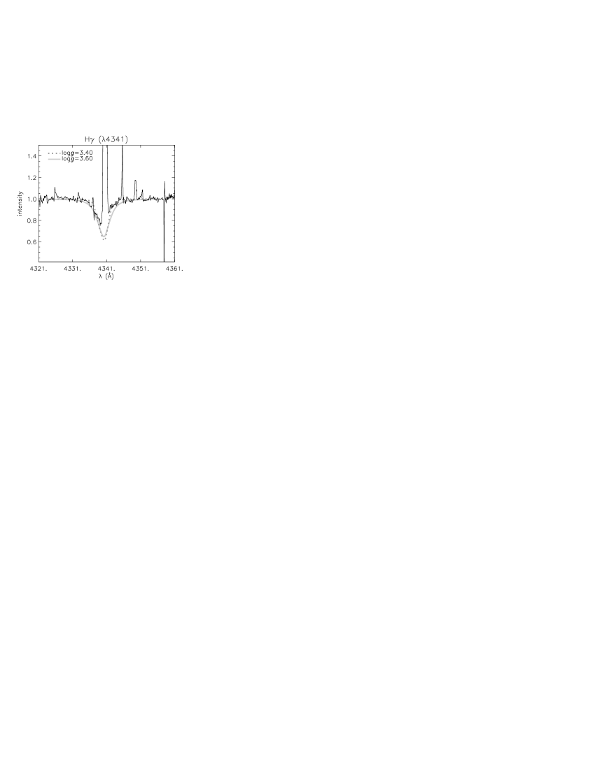
Figure 2: M 2$-$33: H$\gamma$ at different gravities. $T_{\rm\kern-1.04996ptef\kern-0.35002ptf}=39\,000$, $Y_{\rm He}=0.1$, $v\,\sin i=80$ and wind strength as derived from our complete analysis (see Table 3). Note the difficulty in deciding on the best fit.

At first, the line profiles of H$\gamma$ and H$\beta$ were used to determine $\log g$ for the possible range in $T_{\rm\kern-1.04996ptef\kern-0.35002ptf}$ as resulting from our crude estimates. The effect of different gravities on H$\gamma$ is displayed in Figure 2. Then, the effective temperature was derived, from the ratio of He i to He ii, whereas the absolute strengths of the helium lines define the helium abundance, $Y_{\rm He}$. Finally, the wind strength parameter, $\log Q$, and the clumping factor $f_{\rm cl}$ were determined, using all profiles, in particular H$\alpha$ and He ii 4686.

In case of strong mass-loss (well-developed H$\alpha$), $v_{\rm\infty}$ could be determined from the width of H$\alpha$ (we used $v_{\rm\infty}/v_{\rm esc}\approx 2$ to $3$ as a starting point), whereas in cases of weaker $\dot{M}$ the synthetic profile reacts too weakly on variations of $v_{\rm\infty}$ to allow for such a procedure. For these stars $v_{\rm\infty}$ was interpolated from the Table provided by Kudritzki et al. (1997), who used terminal velocities for CSPN of roughly similar parameters derived from UV resonance line profiles.

For all objects, we also checked the available silicon lines for consistency. The corresponding model atom is the same as used and described by Trundle et al. (2004) in their analysis of SMC B supergiants.

3.3 Wind clumping

During our first analysis of the spectra, for two of our objects, M 1$-$38 and M 2$-$12, it was impossible to fit H$\alpha$ and He ii $\lambda$4686 at the same mass-loss rate simultaneously (the predicted He ii emission was by far too large, compared to the observed absorption profiles, see Figure 8, dotted profiles).

Since at that time evidence had accumulated that WR and OB-star winds might be clumped (cf. Puls et al. 2006 and references therein), and since it was to be expected that clumping should affect H$\alpha$ and He ii in a different way for cooler objects, we investigated to what extent this process is able to solve the discussed problem. The assumption of a clumped wind leads to a satisfying solution.

Independent of this work, the same problem and solution was found in the re-analysis of a different sample of CSPN, and a detailed discussion of the involved physics can be found in the corresponding publication (Kudritzki et al., 2006). In brief, and as outlined above, small-scale clumping preserves the profiles of $\rho^{2}$-dependent lines, as long as the apparent mass-loss rate, $\dot{M}\sqrt{f_{\rm cl}}$, remains constant. Though for almost the complete OB star range H$\alpha$ follows this scaling (since H i is a trace ion), He ii becomes the dominant ion (or close to this) for late O-type objects, and the corresponding opacities scale (almost) linearly with density. In such a case then, the corresponding line profiles (in particular, He ii $\lambda$4686) do not react on wind-clumping, but depend on the actual mass-loss rate, $\dot{M}$, alone. Thus, a clumped wind with a mass-loss rate lower than derived from unclumped models can explain that He ii $\lambda$4686 is still in absorption (because the actual mass-loss rate is low), whereas the strong emission in H$\alpha$ is a consequence of clumping. Figure 8 illustrates this behavior, where the solid grey profiles have been calculated with a mass-loss rate reduced by a factor of $\sqrt{f_{\rm cl}}$ (compared to the dotted solution), and a clumped wind with $f_{\rm cl}=30$ has been assumed. Note that all other lines analyzed here react only weakly to the presence/absence of clumping, either because they are formed very close to the photosphere, or because they are also dependent on $\rho^{2}$ (such as He i at cooler temperatures).

Two additional comments: (i) For hotter objects ($T_{\rm\kern-1.04996ptef\kern-0.35002ptf}\ga$ 35…38 kK, depending on gravity), He iii becomes the dominant ion, and both H$\alpha$ and He ii $\lambda$4686 depend on the apparent mass-loss rate. In such a case, the comparison of both lines does not allow us to conclude on the degree of clumping. (ii) If the observed H$\alpha$ and He ii $\lambda$4686 lines show a similar degree of emission at cooler temperatures, this strongly suggests that the corresponding wind is unclumped, i.e., $f_{\rm cl}=1$.

3.4 Error estimates for quantities derived from the spectra alone

Thanks to the high quality of our spectra, fitting errors due to resolution limitations or instrumental noise do not play a role in our analysis. The major problem encountered here is the strong contamination of the hydrogen and He i lines by nebular emission in their cores and beyond. In certain cases (particularly in H$\alpha$, e.g. M 1$-$37 and M 1$-$38) the contamination is so severe that the uncertainties in the derived parameters depend mainly on our inability to identify the stellar profile unambiguously.

Apart from this principal problem, the second major source of errors is due to our “eye-fit” procedure (contrasted to automated methods, e.g., Mokiem et al. 2005), which in certain cases might not be able to find the global optimum in parameter space. Because of the severe nebular contamination, however, an automated method is very difficult to apply, due to the problems of defining the “true” stellar spectrum required for such a procedure.

In the following, we will summarize the typical errors resulting from our spectral analysis. Errors of quantities related to other diagnostics (masses, radii, distances and absolute mass-loss rates) will be discussed in Section 4.

3.4.1 Effective temperatures

Depending on the quality of the helium line fits and the nebula contamination, the typical formal errors in $T_{\rm\kern-1.04996ptef\kern-0.35002ptf}$ are about $\pm 1\,500$ K. This uncertainty becomes larger in the region around $T_{\rm\kern-1.04996ptef\kern-0.35002ptf}=32\,000{\ldots}36\,000$ K, if we account for the (known) problem of a possible inconsistency between the predicted line-strengths of He i triplets and singlets (due to subtle line overlap effects regarding the He i resonance line in the FUV, see Najarro et al. 2006). In this temperature range, the triplet lines are the more reliable ones (see also Mokiem et al. 2005), and are consequently used as a main indicator for the determination of $T_{\rm\kern-1.04996ptef\kern-0.35002ptf}$.

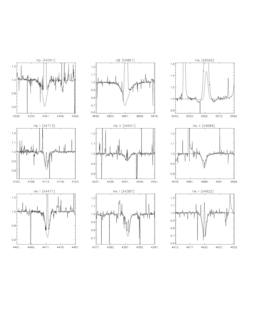
Figure 3: He 2$-$260: H and He i/He ii lines analyzed in this study, together with the predictions from our best fitting model (grey).

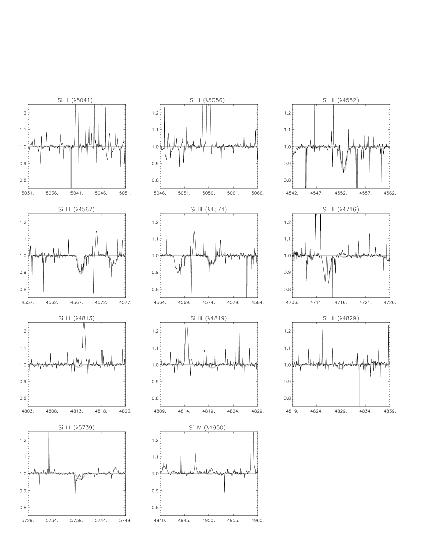
Figure 4: He 2$-$260: important Si lines present in our data set. Overplotted are the theoretical predictions for identical parameters as used in Figure 3 (solar Si abundance).

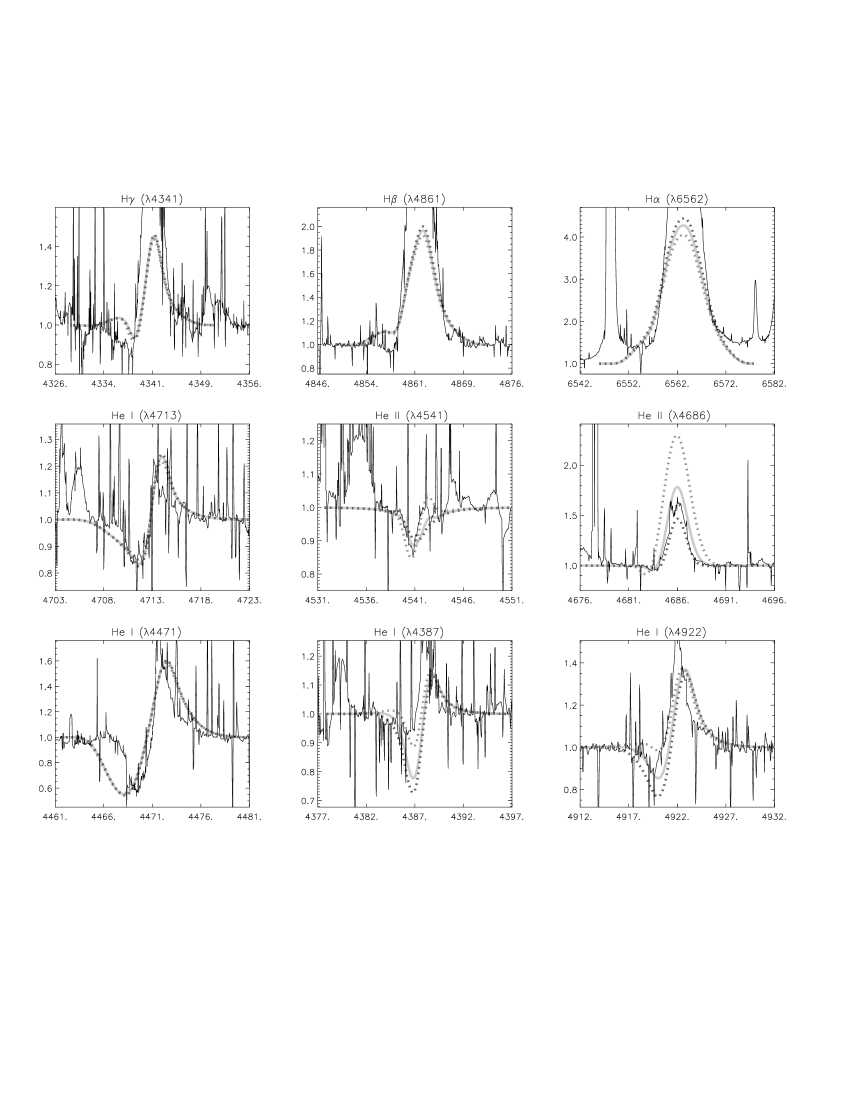
Figure 5: As Figure 3, but for M 1$-$37. The dotted profiles refer to models with different gravities, $\Delta\log g=\pm 0.3$ (stronger emission in He ii$\lambda$4686 for decreased gravity, see text).

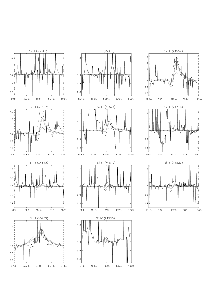
Figure 6: As Figure 4, but for M 1$-$37. A silicon abundance of roughly 30 times the solar one has to be adopted in order to reproduce the observations. Again, the dotted profiles refer to models with different gravities, $\Delta\log g=\pm 0.3$.

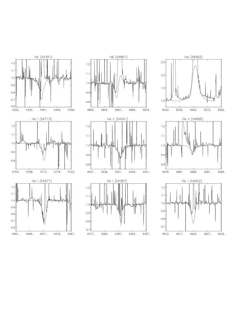
Figure 7: As Figure 3, but for M 1$-$38.

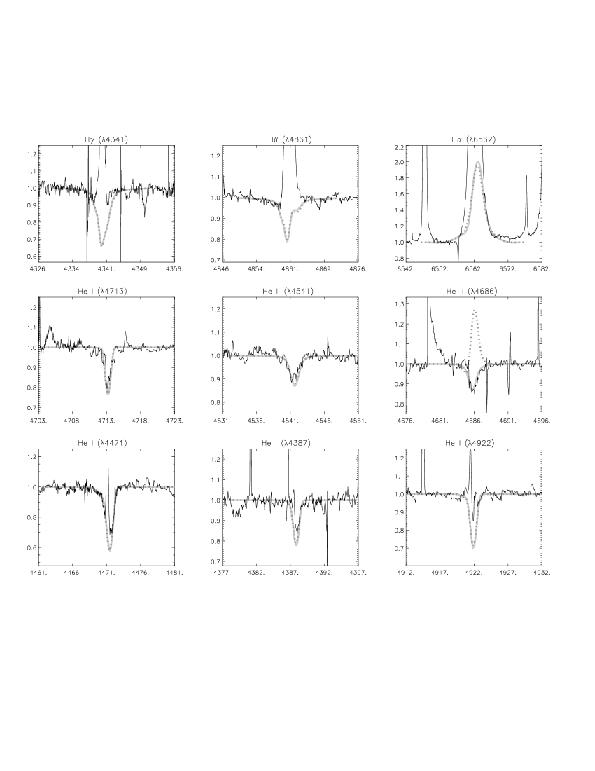
Figure 8: As Figure 3, but for M 2$-$12. The dotted profiles display the predictions from an unclumped model at larger mass-loss rate. Note that the only difference regards He ii $\lambda$4686 (see Section 3.3).

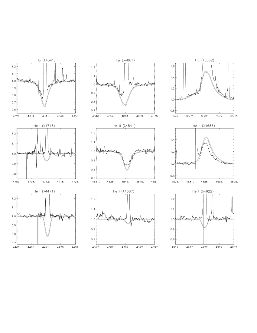
Figure 9: As Figure 3, but for M 2$-$33. The dotted profiles refer to a clumped model with $f_{\rm cl}=7$ (see text).

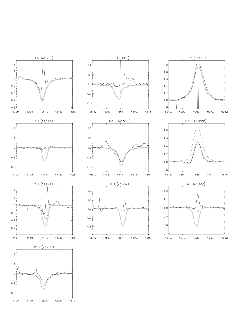
Figure 10: He 2$-$108, H and He line fits. Note the lower quality of the observed spectra, compared to the other objects. Solid: low $T_{\rm\kern-1.04996ptef\kern-0.35002ptf}$ solution, for an unclumped model and a mass-loss rate required to fit H$\alpha$ and He ii $\lambda$4686. Dotted: high $T_{\rm\kern-1.04996ptef\kern-0.35002ptf}$ solution, again for an unclumped model designed to match H$\alpha$. (see text).

3.4.2 Gravities

Because of the intrinsic coupling of $\log g$ and $T_{\rm\kern-1.04996ptef\kern-0.35002ptf}$ when deriving the gravity from the Balmer line wings (typically, a change by 1000 K corresponds to change in $\log g$ by 0.1, in the same direction), the precision of $\log g$ (which is of major importance in the present investigation) depends strongly on the precision of $T_{\rm\kern-1.04996ptef\kern-0.35002ptf}$ (from the He ionization balance) which in turn requires a reasonable determination of the helium abundance, $Y_{\rm He}$. With respect to the available spectra and their nebular contamination, this may not be warranted in all cases. Particularly for He 2-108, the uncertainties were large enough to persuade us to provide two different solutions for this object, at lower and higher $T_{\rm\kern-1.04996ptef\kern-0.35002ptf}$ (for details, see Section 3.5.6).

In most other cases, we adopt, in accordance with similar investigations, a typical error of $\Delta\log g=\pm 0.1$, since for larger differences the profile shape changes significantly. If the star is close to the Eddington limit, the effective gravity becomes smaller and smaller because of the increased radiation pressure (not only from Thomson scattering, but also from photospheric line pressure). The “true” gravity is given by $g_{\rm grav}=g_{\rm eff}+g_{\rm rad}$ (excluding centrifugal forces for the moment, but see Section 4.1.1), where the Balmer line wings actually “measure” $g_{\rm eff}$ because of their dependence on the electron density. As soon as $g_{\rm rad}\ga g_{\rm eff}$, any uncertainty in the calculated radiation pressure (intrinsic to the atmospheric models and strongly dependent on the completeness of the line list) results in a larger error for $g_{\rm grav}$, which we adopt in these cases by $\Delta\log g=0.15$.

3.4.3 Wind parameters

As outlined above, terminal velocities were derived, where possible, from the width of H$\alpha$. Particularly, we found $v_{\rm\infty}=500\pm 100$ km/s for M 1$-$37, and $v_{\rm\infty}=800\pm 160$ km/s for M 2$-$33. Strictly speaking, both values can be considered as lower limits only. For the other objects we adopted $v_{\rm\infty}$ from interpolating between “known” terminal velocities measured for different samples (cf. Kudritzki et al. 1997), and allowed for typical errors of 20%.

The precision of the wind-strength parameter, $\log Q$, on the other hand, depends on the validity of the derived velocity exponents, $\beta$ (Puls et al., 1996). To account for this fact, we have fitted $\log Q$ for different values of $\beta\pm\Delta\beta$, with $\Delta\beta=0.1$. In this case then, $\Delta\log Q$ is typically not larger than $\pm 0.1$ (see also Markova et al. 2004 and Repolust et al. 2004).

3.5 Comments on the individual objects

In the following, we compare our best fitting synthetic spectra with the observed ones, for all H and He lines which have been analyzed. For two of our objects, He 2$-$260 and M 1$-$37, the Si line “fits” are displayed as well. Whereas for all but one of our objects the Si lines matched nicely the observations at solar abundance (with He 2$-$260 being a prototypical object in this respect), we found a very large Si-abundance for M 1$-$37, which is still lacking any theoretical explanation.

Note that all of our objects display a rather strong H$\alpha$ emission, immediately pointing to large wind-strengths (cf. Table 3), which indeed are a factor of about 5 to 10 larger than for typical O and B supergiants. Further comments on this behavior are given in Section 4.3.

All results from our analysis including corresponding errors have been summarized in Table 3.

3.5.1 He 2$-$260

For this star, we obtained a convincing fit, displayed in Figures 3 and 4. The observed and synthetic H$\gamma$ lines agree well, i.e., $\log g$ is well determined within the nominal error. The second diagnostics for $\log g$, H$\beta$, would require a slightly larger value, but this would deteriorate not only H$\gamma$ but also He i $\lambda$$\lambda$4387 and 4922 as well as Si iii.

Compared to the other objects, H$\alpha$ shows the lowest emission, which immediately points to a “low” mass-loss rate. Since He ii $\lambda$4686 is closely reproduced in parallel (no clumping required to keep this line in absorption at the derived effective temperature of 28 000 K), and all other lines fit almost perfectly (including silicon, where Si iii is matched at solar abundance, and Si ii and Si iv are absent as predicted) we feel rather confident about the stellar and wind parameters of our model.

3.5.2 M 1$-$37

Although not classified as a Wolf-Rayet star, this star shows well developed P-Cygni profiles in He i (Figure 5) and Si iii (Figure 6), immediately pointing to an extremely dense wind (the densest in our sample).

To fit the He i lines, an enhanced helium abundance of at least $Y_{\rm He}=1.0$ is required, where even larger values cannot be excluded due to saturation effects. For lower helium content, on the other hand, a fit to the He i lines would require a larger mass loss rate, leading to too strong emission in H$\alpha$, H$\beta$ and H$\gamma$.

Although there is some (stellar?) absorption visible in the blue wings of H$\gamma$ and H$\beta$, we were not able to match these features, thus leaving the gravity rather unconstrained: Models calculated with different $\log g$ (and all other parameters kept constant) display only marginal differences in the spectra, which is not surprising since for such large wind-densities all lines are formed in the wind. However, if we changed not only $\log g$ but also $R_{\ast}$ (and $\dot{M}$ to conserve $Q$) according to the core mass-luminosity relation, differences became visible, because not all quantities scale exactly with $Q$ (cf. Puls et al. 2005). The differences for $\Delta\log g=\pm 0.3$ can be seen in Figs. 5 and 6. The largest reaction is found for He ii $\lambda$4686, where the emission becomes stronger with lower $\log g$ and larger $R_{\ast}$. Note, however, that this effect can be compensated by introducing a certain degree of clumping (see below).

As we were not able to derive $\log g$ spectroscopically, we adopted $\log g\approx 3.4$ from distance considerations (assuming that the star is located at $\approx$ 8 kpc). Lower values for $\log g$ would place the star further away, higher values to closer distances. Moreover, we adopt quite a large error of $\Delta\log g=\pm 0.3$, thereby allowing for distances in between 5.3 kpc and 11.5 kpc (see Table 3). This seems to be a reasonable range, comparing with our most distant object, M 2$-$12, located at 11.4 kpc according to our analysis.

The determination of $T_{\rm\kern-1.04996ptef\kern-0.35002ptf}$ from the ratio of He i to He ii provides similar problems as the definition of the other parameters. The adopted value of 31 000 K is an upper limit, depending alone on our fit to He ii $\lambda$4541. A lower limit on $T_{\rm\kern-1.04996ptef\kern-0.35002ptf}$ can be derived from the absence of stellar Si ii lines, which have been found to appear below $T_{\rm\kern-1.04996ptef\kern-0.35002ptf}=29\,000$ K. To fit the Si iii emission lines, an extremely large Si abundance is required (28 times the solar abundance). According to stellar evolution models the Si abundance should not change, even in H-deficient stars (Werner & Herwig, 2006), and we have no explanation for this finding. Leuenhagen & Hamann (1998) claim solar Si abundance for similar objects but mention overabundances (up to 40 times solar) for some [WCL] stars.

Both H$\alpha$ and He ii $\lambda$4686 are consistent with an unclumped wind of the quoted strength, although the complete H$\alpha$ line is hidden within the strong nebular emission. Note that there is no indication of clumping at the derived/adopted parameters of our final model, since the presence of clumping would decrease the He ii emission and require a higher $T_{\rm\kern-1.04996ptef\kern-0.35002ptf}$ to recover the observations, which is inconsistent with the other lines. Nevertheless, (moderate) clumping cannot be excluded, since a lower gravity (compensating for the decreased emission) is still possible. Note also that a clumped wind might be able to decrease the derived Si abundance.

3.5.3 M 1$-$38

All parameters can be derived with a reliable precision within the nominal errors. $\log g$ is well defined from the wings of H$\gamma$ and H$\beta$, and $T_{\rm\kern-1.04996ptef\kern-0.35002ptf}$ and (solar) $Y_{\rm He}$ are equally well constrained from He ii $\lambda$$\lambda$4541/4686 and He i $\lambda$4471. In contrast, however, we could not obtain a satisfying fit for the He i $\lambda$$\lambda$4387/4922 singlets (overestimated strengths, presumably due to the “singlet problem” outlined above), and we have discarded them from our analysis.

This object is the first where we needed a clumped wind, in order to fit H$\alpha$ and He ii $\lambda$4686 simultaneously at the derived effective temperature. Note that all other lines do not react on clumping, but are consistent with the derived “apparent” wind-strength, $\dot{M}\sqrt{f_{\rm cl}}$. This value and the individual quantities for $\dot{M}$ and $f_{\rm cl}\approx 20$ were determined by a compromise to fit the wind-induced asymmetries seen in most lines, the emission profile in H$\alpha$ and the absorption line profile of He ii $\lambda$4686.

3.5.4 M 2$-$12

Both H$\gamma$ and H$\beta$ are dominated by the strong nebular lines, and only the extreme wings become visible. This leads to a higher uncertainty in $\log g$, with an error of $\Delta\log g=+0.2/-0.1$.

As above, the synthetic He i singlets might appear as too strong, but in this case the nebular contamination forbids a reliable estimate on whether this is really the case. From the triplet lines and He ii $\lambda$$\lambda$4541/4686 then, we derive a well defined $T_{\rm\kern-1.04996ptef\kern-0.35002ptf}$ and helium abundance $Y_{\rm He}$, within the nominal errors. We prefer a somewhat reduced helium abundance, $Y_{\rm He}=0.08$, in order to fit the globally weak He-lines.

Again, a clumping factor of $f_{\rm cl}\approx 30$ is required to keep He ii $\lambda$4686 in absorption. Further details on this problem have been outlined in Section 3.3.

3.5.5 M 2$-$33

For this object, the quality of both the spectra and the fits is satisfactory, and nominal errors apply for all parameters except for $T_{\rm\kern-1.04996ptef\kern-0.35002ptf}$ and thus $\log g$ (see Figure 9). Since most of the He i absorption lines are very weak and thus dominated by nebular emission, the ratio of He i to He ii cannot be determined well enough to ascertain the effective temperature precisely. We estimate the corresponding error as $\Delta T_{\rm\kern-1.04996ptef\kern-0.35002ptf}=\pm 2\,000$ K.

Anyway, in this temperature range (roughly 39 000 K) He ii is no longer a dominant ion, and the corresponding opacities scale with $\rho^{2}$. According to our arguments given in Section 3.3, a unique determination of the clumping factor is no longer possible, and we adopt $f_{\rm cl}=1$. A comparison between such an unclumped and a clumped model is given in Figure 9: the dotted profiles refer to a clumped model with $f_{\rm cl}=7$, and the small difference in He ii$\lambda$4686 result from the fact that He iii recombines in the outmost wind ($v/v_{\rm\infty}\geq 0.8$).

3.5.6 He 2$-$108

This object has been previously analyzed in the literature, with two differing values for $T_{\rm\kern-1.04996ptef\kern-0.35002ptf}$ (and related quantities). A low temperature solution with $T_{\rm\kern-1.04996ptef\kern-0.35002ptf}$ = 35 000 K / 34 000 K was deduced by Kudritzki et al. (1997/2006), from the optical, whereas a high temperature solution with $T_{\rm\kern-1.04996ptef\kern-0.35002ptf}$ = 39 000 K was found by Pauldrach et al. (2004), on the basis of the Feiii/iv ionization equilibrium derived from the UV.

Given the low quality of the available spectra, none of these solutions can be excluded. Three of the four available He i lines appear to be weak, thus supporting the high temperature solution, whereas He i $\lambda$4471 seems to be much stronger, thus favoring the lower $T_{\rm\kern-1.04996ptef\kern-0.35002ptf}$. Rather than trying to find a compromise, we decided to show both solutions, and to follow the consequences throughout the remainder of this paper.

Our low temperature solution (Figure 10, solid) has been optimized for He i $\lambda$4471, and results in $T_{\rm\kern-1.04996ptef\kern-0.35002ptf}$ = 34 000 K, identical to the value derived by Kudritzki et al. (2006). In this case, both He i singlets $\lambda$$\lambda$4387/4922 and the He i $\lambda$4713 triplet are overestimated, whereas for the high temperature solution (dotted) it is basically the other way round. Note that the singlets at $T_{\rm\kern-1.04996ptef\kern-0.35002ptf}$ = 34 000 K might be overestimated, due to the singlet problem. At least at $T_{\rm\kern-1.04996ptef\kern-0.35002ptf}$ = 39 000 K, however, this problem is no longer relevant, and the agreement between observed and predicted singlets cannot be disputed.

The errors for our low temperature solution (from He i $\lambda$4471) have been estimated as +1 000/$-$2 000 K for $T_{\rm\kern-1.04996ptef\kern-0.35002ptf}$, and a standard error of $\Delta\log g=0.1$. In this case then, the helium abundance must be slightly enhanced, $Y_{\rm He}=0.15$.

From the simultaneous analysis of the Balmer lines and He ii $\lambda$4686, we found an interesting result on the clumping properties of the wind. In contrast to the other objects, He 2$-$108 seems to require larger clumping factors in the inner wind, compared to the outer one. First, note that, at $T_{\rm\kern-1.04996ptef\kern-0.35002ptf}\ga 34\,000$ K, there is no discrepancy between H$\alpha$ and He ii $\lambda$4686 (in agreement with the discussion given in Section 3.3). In contrast, however, there is now an inconsistency between H$\alpha$ and H$\gamma$/H$\beta$.

For the low temperature solution, we have “normalized” the (unclumped) mass-loss rate to fit H$\alpha$/He ii $\lambda$4686, and obviously the cores of H$\gamma$ and H$\beta$ are predicted as too deep. Thus, clumping must be larger in the inner wind, to allow for a refilling of both lines due to increased emission.

For the high temperature solution, an unclumped model designed to fit H$\alpha$ predicts too much He ii $\lambda$4686 emission (this inconsistency cannot be cured by clumped models, because of the high temperature), and, again, too little emission in H$\gamma$ and H$\beta$.

Note that He 2$-$108 is the only object in our sample which indicates such a stratified clumping. Because in the present analysis we are considering only depth independent clumping (see Section 3.1), we provide (both for the high and the low temperature solution) a clumping factor of unity in Table 3, consistent with the wind-lines, but are aware of the fact that the real mass-loss rate(s) might be smaller than indicated.

4 Deduced Parameters: Masses, radii, distances and wind-momentum rates

Table 3: Results of our analysis for the complete sample, using either “Method 1” or “Method 2” (see text). $\log g_{\rm spec}$ refers to the gravity as derived from spectroscopy, and $\log g_{\rm true}$ is an estimate (upper limit) for the true gravity, corrected for centrifugal acceleration and used to calculate related physical properties. Wind strength parameter $\log Q$ calculated with $\dot{M}$ in units $M_{\odot}$/yr, $v_{\rm\infty}$ in km/s and $R_{\ast}$ in $R_{\odot}$. Modified wind-momentum rate, $D_{\rm mom}$, calculated in cgs. The different distances resulting from “Method 1” refer to the different extinctions as given at the top of the table. All other parameters which are dependent on extinction refer to the “mean” value, $A_{V\,{\rm mean}}$ (see text).

Object name	He 2$-$260	M 1$-$37∗∗∗	M 1$-$38	M 2$-$12	M 2$-$33	He 2$-$108	He 2$-$108
PN G	$008.2+06.8$	$002.6-03.4$	$002.4-03.7$	$359.8+05.6$	$002.0-06.2$	$316.1+08.4$	$316.1+08.4$
$V$ (mag)	$14.27\pm 0.10$	$14.99\pm 0.25$	$14.45\pm 0.25$	$14.74\pm 0.10$	$14.40\pm 0.50$	$12.63\pm 0.10$	$12.63\pm 0.10$
$A_{V\leavevmode\nobreak\ {\rm optical}}$   (mag)	$1.95$	$2.49$	$2.62$	$2.55$	$1.06$	$1.30$	$1.30$
$A_{V\leavevmode\nobreak\ {\rm radio}}$   (mag)	$1.57$	$1.57$	$1.81$	$1.81$	$0.42$	$0.94$	$0.94$
$A_{V\leavevmode\nobreak\ {\rm mean}}\,^{*}$ (mag)	$1.76\pm 0.19$	$2.03\pm 0.46$	$2.21\pm 0.41$	$2.18\pm 0.37$	$0.74\pm 0.32$	$1.12\pm 0.18$	$1.12\pm 0.18$
$v_{\rm rad}$ (km/s)	$37\pm 10$	$235\pm 10$	$-75\pm 10$	$110\pm 10$	$-127\pm 10$	$-35\pm 10$	$-35\pm 10$
$v\,\sin i\,^{**}$ (km/s)	$<55\pm 10$	$<70\pm 10$	$<50\pm 10$	$<60\pm 10$	$<80\pm 10$	$<80\pm 10$	$<80\pm 10$
$T_{\rm\kern-1.04996ptef\kern-0.35002ptf}$ (K)	$28000\leavevmode\nobreak\ ^{+1500}_{-1500}$	$31000\leavevmode\nobreak\ ^{+1500}_{-2000}$	$31000\leavevmode\nobreak\ ^{+1500}_{-1500}$	$30500\leavevmode\nobreak\ ^{+1500}_{-1500}$	$39000\leavevmode\nobreak\ ^{+2000}_{-2000}$	$34000\leavevmode\nobreak\ ^{+1000}_{-2000}$	$39000\leavevmode\nobreak\ ^{+1500}_{-1500}$
$\log g_{\rm spec}$	$2.90\leavevmode\nobreak\ ^{+0.10}_{-0.10}$	$3.40\leavevmode\nobreak\ ^{+0.30}_{-0.30}$	$3.05\leavevmode\nobreak\ ^{+0.10}_{-0.10}$	$3.00\leavevmode\nobreak\ ^{+0.20}_{-0.10}$	$3.60\leavevmode\nobreak\ ^{+0.15}_{-0.15}$	$3.50\leavevmode\nobreak\ ^{+0.10}_{-0.10}$	$3.70\leavevmode\nobreak\ ^{+0.10}_{-0.10}$
$\log g_{\rm true}$	$2.95\leavevmode\nobreak\ ^{+0.09}_{-0.09}$	$3.45\leavevmode\nobreak\ ^{+0.27}_{-0.27}$	$3.08\leavevmode\nobreak\ ^{+0.09}_{-0.09}$	$3.05\leavevmode\nobreak\ ^{+0.18}_{-0.09}$	$3.65\leavevmode\nobreak\ ^{+0.14}_{-0.14}$	$3.56\leavevmode\nobreak\ ^{+0.09}_{-0.09}$	$3.74\leavevmode\nobreak\ ^{+0.09}_{-0.09}$
$Y_{\rm He}$ ($=N_{\rm He}/N_{\rm H}$)	$0.10\pm 0.02$	$1.00\pm 0.50$	$0.10\pm 0.02$	$0.08\pm 0.02$	$0.10\pm 0.02$	$0.15\pm 0.02$	$0.10\pm 0.02$
$\log Q$	$-12.3\pm 0.1$	$-10.9\pm 0.1$	$-12.3\pm 0.1$	$-12.6\pm 0.1$	$-11.7\pm 0.1$	$-11.7\pm 0.1$	$-11.7\pm 0.1$
$f_{\rm cl}$	$1$	$1$	$20$	$30$	$1$	$1$	$1$
$\beta$	$2.5\pm 0.1$	$3.0\pm 0.5$	$1.5\pm 0.1$	$1.5\pm 0.1$	$1.0\pm 0.1$	$1.2\pm 0.1$	$1.5\pm 0.1$
$v_{\rm\infty}$ (km/s)	$450\pm 90$	$600\pm 120$	$450\pm 90$	$450\pm 90$	$800\pm 160$	$700\pm 70$	$700\pm 70$
Method 1 ∗
$M_{\rm evol}$ ($M_{\odot}$)	$0.71\leavevmode\nobreak\ ^{+0.13}_{-0.06}$	$0.58\leavevmode\nobreak\ ^{+0.09}_{-0.06}$	$0.77\leavevmode\nobreak\ ^{+0.11}_{-0.10}$	$0.78\leavevmode\nobreak\ ^{+0.10}_{-0.16}$	$0.64\leavevmode\nobreak\ ^{+0.09}_{-0.05}$	$0.59\leavevmode\nobreak\ ^{+0.02}_{-0.02}$	$0.60\leavevmode\nobreak\ ^{+0.03}_{-0.02}$
$R_{\rm evol}$ ($R_{\odot}$)	$4.69\leavevmode\nobreak\ ^{+0.68}_{-0.51}$	$2.38\leavevmode\nobreak\ ^{+0.89}_{-0.64}$	$4.19\leavevmode\nobreak\ ^{+0.56}_{-0.50}$	$4.38\leavevmode\nobreak\ ^{+0.57}_{-0.92}$	$1.99\leavevmode\nobreak\ ^{+0.37}_{-0.30}$	$2.13\leavevmode\nobreak\ ^{+0.24}_{-0.22}$	$1.73\leavevmode\nobreak\ ^{+0.20}_{-0.18}$
$\log\,(L/L_{\odot})$	$4.09\leavevmode\nobreak\ ^{+0.15}_{-0.14}$	$3.68\leavevmode\nobreak\ ^{+0.29}_{-0.30}$	$4.17\leavevmode\nobreak\ ^{+0.14}_{-0.14}$	$4.18\leavevmode\nobreak\ ^{+0.13}_{-0.22}$	$3.92\leavevmode\nobreak\ ^{+0.17}_{-0.17}$	$3.74\leavevmode\nobreak\ ^{+0.10}_{-0.14}$	$3.80\leavevmode\nobreak\ ^{+0.11}_{-0.12}$
$\dot{M}$ ($M_{\odot}$/yr)	$0.45\times 10^{-7}$	$7.63\times 10^{-7}$	$0.40\times 10^{-7}$	$0.24\times 10^{-7}$	$1.13\times 10^{-7}$	$1.07\times 10^{-7}$	$0.92\times 10^{-7}$
$\log\,D_{\rm mom}$	$26.44\leavevmode\nobreak\ ^{+0.25}_{-0.24}$	$27.65\leavevmode\nobreak\ ^{+0.35}_{-0.35}$	$26.37\leavevmode\nobreak\ ^{+0.25}_{-0.25}$	$26.15\leavevmode\nobreak\ ^{+0.25}_{-0.30}$	$26.91\leavevmode\nobreak\ ^{+0.27}_{-0.26}$	$26.84\leavevmode\nobreak\ ^{+0.17}_{-0.17}$	$26.73\leavevmode\nobreak\ ^{+0.17}_{-0.17}$
$d_{\rm optical}$ (kpc)	$10.3\leavevmode\nobreak\ ^{+3.8}_{-2.7}$	$6.3\leavevmode\nobreak\ ^{+3.5}_{-2.2}$	$7.9\leavevmode\nobreak\ ^{+3.0}_{-2.2}$	$9.6\leavevmode\nobreak\ ^{+3.4}_{-3.0}$	$8.8\leavevmode\nobreak\ ^{+4.3}_{-2.9}$	$3.4\leavevmode\nobreak\ ^{+1.2}_{-0.9}$	$3.0\leavevmode\nobreak\ ^{+1.1}_{-0.8}$
$d_{\rm radio}$ (kpc)	$12.2\leavevmode\nobreak\ ^{+4.5}_{-3.2}$	$9.6\leavevmode\nobreak\ ^{+5.3}_{-3.4}$	$11.5\leavevmode\nobreak\ ^{+4.4}_{-3.2}$	$13.6\leavevmode\nobreak\ ^{+4.9}_{-4.2}$	$11.9\leavevmode\nobreak\ ^{+5.8}_{-3.9}$	$4.0\leavevmode\nobreak\ ^{+1.4}_{-1.0}$	$3.6\leavevmode\nobreak\ ^{+1.3}_{-0.9}$
$d_{\rm mean}$ (kpc)	$11.2\leavevmode\nobreak\ ^{+2.0}_{-1.6}$	$7.8\leavevmode\nobreak\ ^{+3.8}_{-2.6}$	$9.6\leavevmode\nobreak\ ^{+2.8}_{-2.2}$	$11.5\leavevmode\nobreak\ ^{+2.8}_{-2.9}$	$10.3\leavevmode\nobreak\ ^{+3.9}_{-2.8}$	$3.7\leavevmode\nobreak\ ^{+0.6}_{-0.5}$	$3.3\leavevmode\nobreak\ ^{+0.5}_{-0.4}$
Method 2 ∗
$d_{\rm adopted}$ (kpc)	$8.0\leavevmode\nobreak\ ^{+2.0}_{-2.0}$	$8.0\leavevmode\nobreak\ ^{+2.0}_{-2.0}$	$8.0\leavevmode\nobreak\ ^{+2.0}_{-2.0}$	$8.0\leavevmode\nobreak\ ^{+2.0}_{-2.0}$	$8.0\leavevmode\nobreak\ ^{+2.0}_{-2.0}$	$4.6\leavevmode\nobreak\ ^{+1.1}_{-1.1}$	$4.6\leavevmode\nobreak\ ^{+1.1}_{-1.1}$
$R_{\rm dist}$ ($R_{\odot}$)	$3.36\leavevmode\nobreak\ ^{+1.06}_{-0.81}$	$2.44\leavevmode\nobreak\ ^{+1.03}_{-0.72}$	$3.51\leavevmode\nobreak\ ^{+1.41}_{-1.01}$	$3.06\leavevmode\nobreak\ ^{+1.12}_{-0.82}$	$1.55\leavevmode\nobreak\ ^{+0.71}_{-0.49}$	$2.64\leavevmode\nobreak\ ^{+0.83}_{-0.63}$	$2.41\leavevmode\nobreak\ ^{+0.76}_{-0.58}$
$M_{\rm dist}$ ($M_{\odot}$)	$0.38\leavevmode\nobreak\ ^{+0.30}_{-0.17}$	$0.61\leavevmode\nobreak\ ^{+0.95}_{-0.37}$	$0.55\leavevmode\nobreak\ ^{+0.57}_{-0.28}$	$0.40\leavevmode\nobreak\ ^{+0.44}_{-0.19}$	$0.40\leavevmode\nobreak\ ^{+0.51}_{-0.22}$	$0.89\leavevmode\nobreak\ ^{+0.72}_{-0.40}$	$1.14\leavevmode\nobreak\ ^{+0.91}_{-0.51}$
$\log\,(L/L_{\odot})$	$3.80\leavevmode\nobreak\ ^{+0.26}_{-0.26}$	$3.70\leavevmode\nobreak\ ^{+0.32}_{-0.33}$	$4.01\leavevmode\nobreak\ ^{+0.31}_{-0.31}$	$3.86\leavevmode\nobreak\ ^{+0.28}_{-0.29}$	$3.70\leavevmode\nobreak\ ^{+0.34}_{-0.34}$	$3.93\leavevmode\nobreak\ ^{+0.24}_{-0.26}$	$4.08\leavevmode\nobreak\ ^{+0.25}_{-0.25}$
$\log\,D_{\rm mom}$	$26.15\leavevmode\nobreak\ ^{+0.33}_{-0.33}$	$27.67\leavevmode\nobreak\ ^{+0.38}_{-0.38}$	$26.21\leavevmode\nobreak\ ^{+0.37}_{-0.37}$	$25.83\leavevmode\nobreak\ ^{+0.35}_{-0.35}$	$26.69\leavevmode\nobreak\ ^{+0.39}_{-0.39}$	$27.03\leavevmode\nobreak\ ^{+0.28}_{-0.28}$	$27.02\leavevmode\nobreak\ ^{+0.28}_{-0.28}$
∗ see text     ∗∗ upper limit, since $v_{\rm macro}$ not measurable     ∗∗∗ $\log g_{\rm spec}$ adopted, see text

4.1 Two different methods

Having presented those results that can be derived from spectroscopy alone, we will concentrate now on the “remaining” parameters that are not directly deducible from our analysis, since they depend on the stellar radius, $R_{\ast}$. Two different, independent approaches will be applied to obtain these parameters: “Method 1” uses evolutionary tracks for central stars to provide masses, which, together with $\log g$, result in stellar radii and finally spectroscopic distances. “Method 2”, on the other hand, uses adopted (bulge-)distances to calculate radii and depending quantities. We will give a detailed error analysis and compare the results and inherent uncertainties of both methods. This will in particular clarify (at least for our sample of objects) the question raised in Section 1, namely in how far the combination of post-AGB evolution theory and state-of-the-art model atmospheres can successfully predict distances from high-resolution spectroscopy.

So far, the spectroscopically determined gravities (from the Balmer-line wings, denoted by $\log g_{\rm spec}$ in Table 3) are effective values, since centrifugal forces lead to an outward acceleration of the atmospheric layers, thus reducing the “true” gravity, $\log g_{\rm true}$. In order to obtain this quantity (which has to be used in our subsequent analysis), we have to correct $\log g_{\rm spec}$ by adding the centrifugal acceleration. This has been accomplished in the “usual” way by means of the derived projected rotational velocities, $v\sin i$, and the average value of $\sin i$ (for details, see Appendix in Repolust et al. 2004 and references therein). As already outlined in Section 3.2, due to missing metallic lines the macro-turbulent velocity, $v_{\rm macro}$, was not measurable for our sample, which means that the quoted values of $v\sin i$ and thus the true gravities have to be considered as upper limits. Note, however, that despite the rather low rotational speeds the differences between $\log g_{\rm spec}$ and $\log g_{\rm true}$ are quite significant (of the order of 0.05 dex), which is due to the small radii of our objects (centrifugal acceleration $\propto v_{\rm rot}^{2}/R_{\ast}$).

4.1.1 Method 1

Figure 11: The positions of the CSPN in the $\log T_{\rm\kern-1.04996ptef\kern-0.35002ptf}-\log g$ diagram, with error bars according to the derived uncertainties, together with theoretical post-AGB evolutionary tracks for stars of five different masses (from Bloecker 1995 and Schönberner 1989, masses in units of $M_{\odot}$). $L$, $H$, $K$ and $P$ denote various results for He 2$-$108: our low and high temperature solution, the analysis by Kudritzki et al. (2006) and by Pauldrach et al. (2004). Remember that the gravity of M 1$-$37 has been adopted.

Here we apply the method to derive spectroscopic distances as described by Méndez et al. (1988b). We use the evolutionary tracks in the $\log T_{\rm\kern-1.04996ptef\kern-0.35002ptf}$-$\log g$ diagram for CSPN from Bloecker (1995) and Schönberner (1989) (Figure 11), which defines the stellar mass, $M_{\ast}$, by interpolating the spectroscopically determined $T_{\rm\kern-1.04996ptef\kern-0.35002ptf}$ and $\log g_{\rm true}$ values between the evolutionary tracks of different masses. This method is feasible for CSPN that are in the phase of almost constant luminosity, because the evolutionary tracks for different masses are unique in this regime.

Since the centrifugal correction term involves the stellar radius, an iterative scheme is required: starting with some guess for $R_{\ast}$, we obtain $M_{\ast}$, a new radius via $\log g_{\rm true}$, which is updated subsequently and a new mass derived. The iteration process is continued until mass and radius have converged. In Table 3, we provide these converged quantities and the corresponding true gravities. Note that the masses and radii derived in this way depend on the validity of the tracks (and on the accuracy of the spectroscopic analysis), but $\it not$ on the extinction.

4.1.2 Method 2

Here we exploit the fact that the observed objects are supposed to be located in the Galactic bulge, following our selection criteria (Section 2). We adopt the well-defined distance to the Galactic center, $R_{0}$, of roughly 8 kpc (7.94 $\pm$ 0.42 kpc, Eisenhauer et al. 2003) for all our objects, except for He 2$-$108.

For the latter one, we adopt a distance of 4.6 kpc, which is consistent with the value provided by Méndez et al. (1992, and also ), 5.8 …6 kpc, if we account for “our” extinction ($A_{V\,{\rm mean}}$, see below) and visual magnitude $V$, together with their stellar parameters. Admittedly, this distance is far from being as well determined as $R_{0}$, and moreover it has been determined by using “Method 1”. In so far, the corresponding results should be considered as a comparison rather than a test.

To check the error propagation of “Method 2” and to compare it with “Method 1”, in all cases we adopt a typical error of 25% in the distance, which accounts for the depth of the Galactic bulge and follows the considerations by Méndez et al. (1988b).

From the distances, the visual magnitude, $V$ (cf. Table 3, all from Tylenda et al. 1991) and the extinction, $A_{V}$ (see below), we find the absolute magnitude, $M_{V}$, which together with the theoretical V-band fluxes (convolved with the corresponding filter transmission function) allows us to derive the stellar radius, $R_{\ast}$, following Kudritzki (1980, see also Eqs. (1,2) in ). The errors inherent to all related quantities (mass, luminosity etc.) are thus dominated by the uncertainty in distance and extinction, except for M 2$-$33, where the large uncertainty in $V$ becomes decisive.

4.1.3 Extinction

As outlined in the introduction, Stasinska et al. (1992) concluded, from a comparison of Balmer decrement extinctions versus radio-H$\beta$ extinctions, that for most distant PN the corresponding line of sight extinction law should be significantly different from the standard law (for the diffuse ISM). They argued that the ratio $R_{V}$ of total to selective extinction (in the V-band) must be lower than the canonical value of 3.1, of the order of $R_{V}$ = 2.7. Similar conclusions were reached more recently by Udalski (2003) and Ruffle et al. (2004).

Using previous results by Seaton (1979), the standard visual extinction can be related to the logarithmic extinction at H$\beta$ determined from the Balmer decrement, $C_{\rm opt}$, via

$$A_{V\,{\rm optical}}=2.16\,C_{\rm opt}\qquad(\mbox{``standard'' reddening}).$$ (3)

The measurements of $C_{\rm rad}$ (the logarithmic extinction at H$\beta$ determined from the radio fluxes) for a large sample of PN by Stasinska et al., on the other hand, imply $R_{V}=2.63$ (using the relations provided by Nandy et al. 1975) and finally

$$A_{V\,{\rm radio}}=2.10\,C_{\rm rad}\qquad(\mbox{lower reddening for distant PN}).$$ (4)

For all our objects, $C_{\rm opt}>C_{\rm rad}$ (values taken from Stasinska et al. and Tylenda et al. 1992), and we have used both the standard reddening to obtain $A_{V\,{\rm optical}}$ and the lower value $A_{V\,{\rm radio}}$ in our further investigations to estimate a maximum and minimum effect. Moreover, we have used also a linear mean, $A_{V\,{\rm mean}}=0.5\leavevmode\nobreak\ (A_{V\,{\rm optical}}+A_{V\,{\rm radio}})$, with larger errors to account for the present uncertainties. In Table 3, we display the different distances determined by “Method 1” resulting from these three values of $A_{V}$, whereas, for brevity, we display only the solutions relying on $A_{V\,{\rm mean}}$ for “Method 2”.

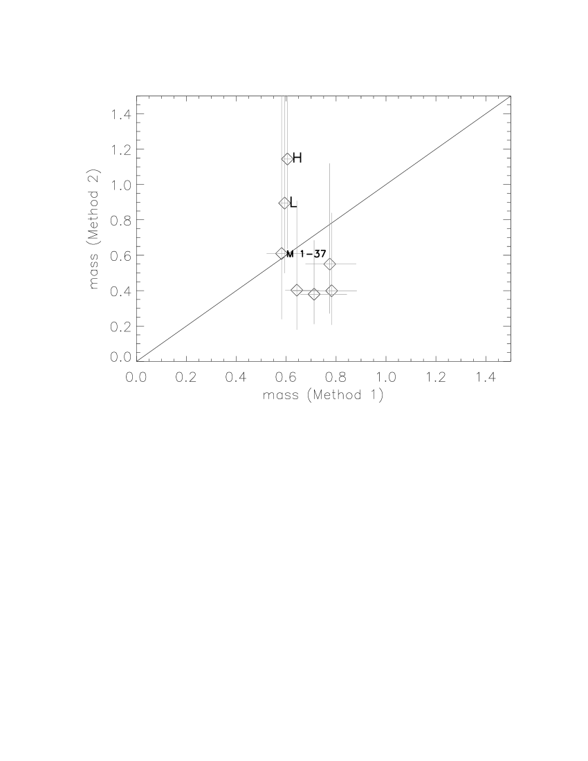
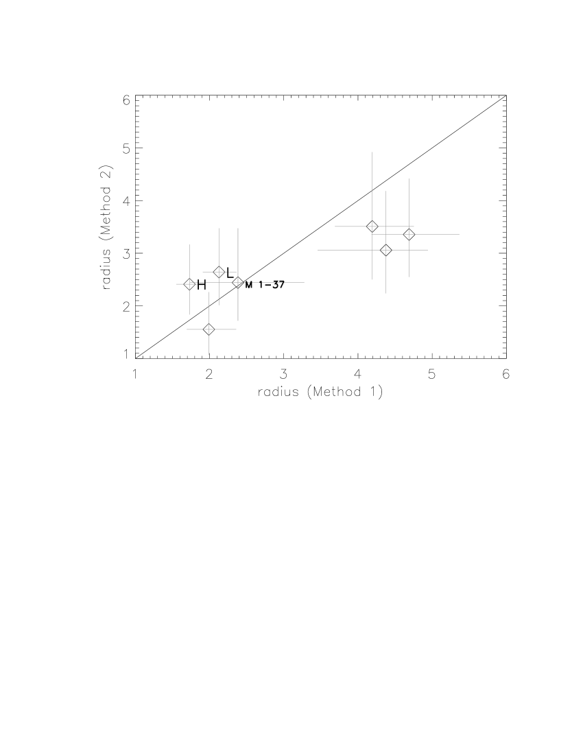
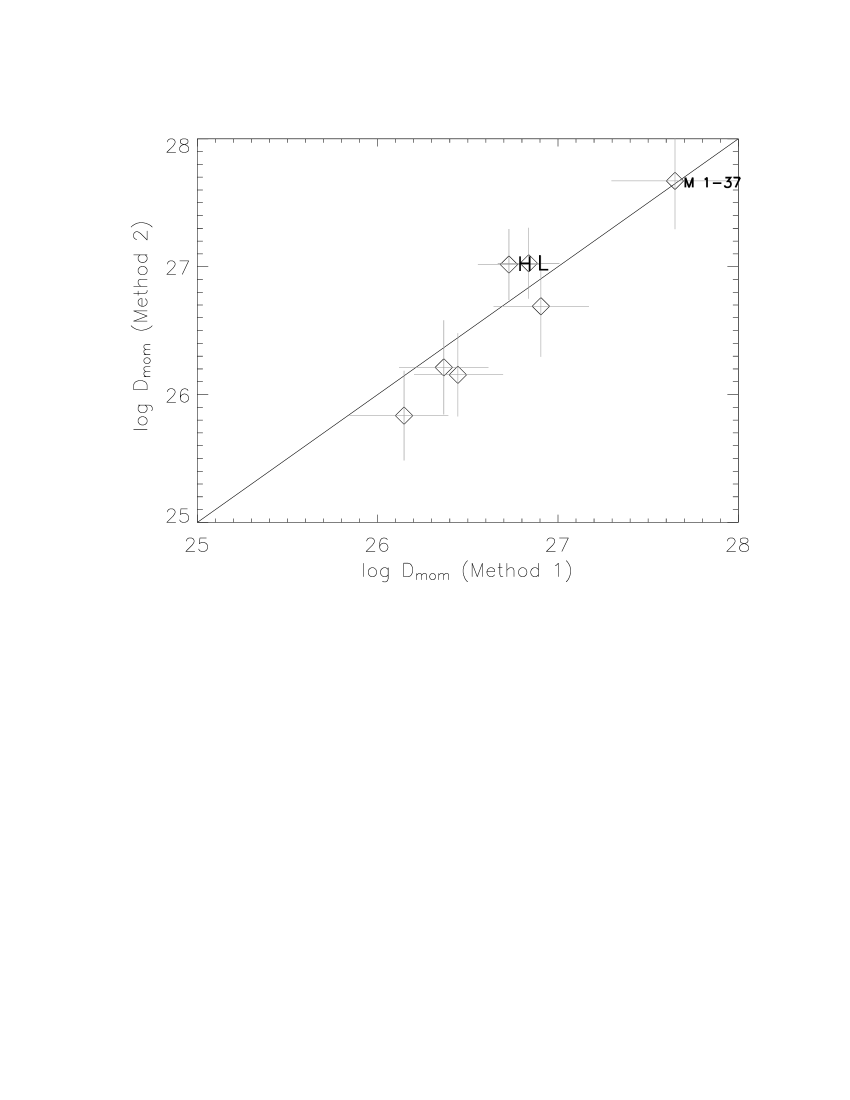
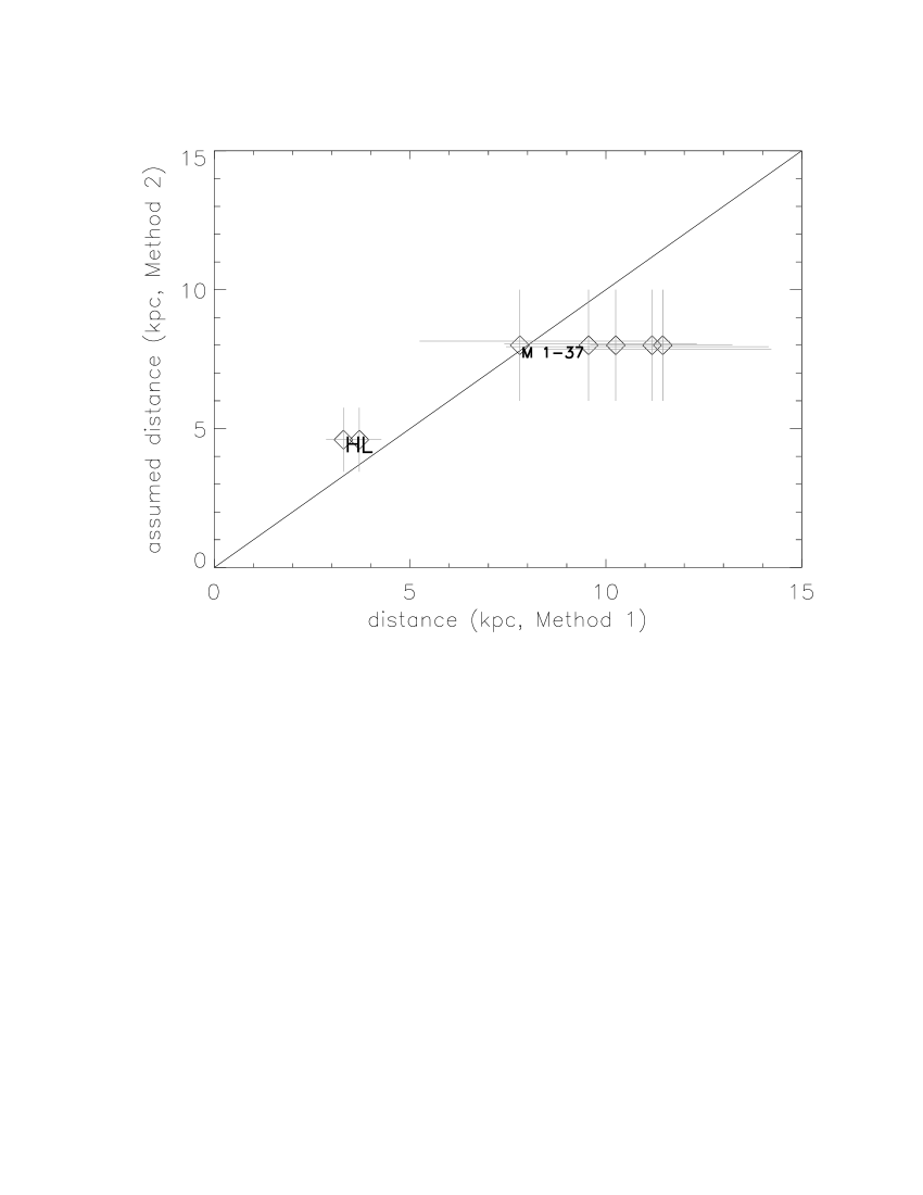
Figure 12: Comparison of various parameters of our CSPN sample, derived by “Method 1” (based on evolutionary tracks) and “Method 2” (based on adopted distances), using the “mean” extinction, $A_{V\,{\rm mean}}$ (see text): masses in units of $M_{\odot}$, radii in $R_{\odot}$, modified wind-momenta in cgs and distances in kpc. $L$ and $H$ refer to the low and high temperature solution for He 2$-$108, respectively. The solid line displays the one-to-one relation. Note that most of the results agree within the error bars, but that the errors inherent to “Method 1” are considerably lower than those relying on “Method 2”. Since the gravity of M 1$-$37 has been adopted from distance arguments, all parameters agree by definition.

4.2 Comparison of Method 1 and 2: stellar parameters and distances

Regarding the error propagation of the quantities observed or determined directly from the spectra (see first part of Table 3) into deduced physical quantities such as radius, mass, luminosity and mass-loss dependent quantities we refer the reader to the detailed discussion provided by Markova et al. (2004) and Repolust et al. (2004).

4.2.1 Mass and radius related quantities

Figure 12 (upper left panel) shows a comparison of the derived masses from the two methods. Obviously, the error bars from “Method 1” are much smaller than those resulting from “Method 2”, which of course is related to the fact that “Method 2” involves the rather large uncertainties in $R_{\ast}$ (due to uncertainties in distance and extinction), but, even more, because $M_{\ast}$ depends quadratically on radius. In contrast, for masses based on evolutionary tracks the dependence on errors in $\log g$ and $T_{\rm\kern-1.04996ptef\kern-0.35002ptf}$ should be minor since the slope of the tracks is fairly parallel to the $T_{\rm\kern-1.04996ptef\kern-0.35002ptf}$-$\log g$ iso-contours of equivalent width for the Balmer lines formed in the photosphere.

Relying on this notion, we defined the mass uncertainty resulting from the adopted errors in $\log g$ and $T_{\rm\kern-1.04996ptef\kern-0.35002ptf}$ in the following way: We determine $M_{\ast}$ for the pair ($\log g+\Delta\log g$, $T_{\rm\kern-1.04996ptef\kern-0.35002ptf}$) as well as for the pair ($\log g$, $T_{\rm\kern-1.04996ptef\kern-0.35002ptf}+\Delta T_{\rm\kern-1.04996ptef\kern-0.35002ptf}$), and use the higher of both masses as our upper limit for $M_{\ast}$. The lower limit is defined analogously, with opposite signs. We do not use combinations of ($+\Delta\log g$, $-\Delta T_{\rm\kern-1.04996ptef\kern-0.35002ptf}$) and vice versa, since such combinations can be excluded from the results of our analysis (remember that the errors in $T_{\rm\kern-1.04996ptef\kern-0.35002ptf}$ and $\log g$ are not independent).

The resulting uncertainties for $M_{\ast}$ are amazingly small; even the object with very large uncertainties in $\log g$, M 1$-$37, has a fairly well determined mass, which is also related to the fact that for lower masses the dependence of $M_{\ast}$ on gravity is rather low. The mass range within our sample extends from 0.58 to 0.78 $M_{\odot}$, with errors of about 15%.

From these results, however, one might also argue that our sample is not completely representative. This is best seen from the fact that the mean stellar mass of our sample is about $0.68M_{\odot}$, which is considerably larger than the expected $0.6M_{\odot}$ (see, e.g., Liebert et al. 2005). Such a discrepancy might be due to selection effects, because for our analysis we choose only objects with a high enough signal to noise ratio. With such a bias towards more luminous objects, we might have selected also the more massive ones.

In contrast, using “Method 2”, the masses are determined from the radius which enters quadratically and is dominated by the large uncertainties in distance and extinction or visual magnitude. If we consider the corresponding errors as already discussed and summarized in Table 3, we find errors in between 30% to 45% for $R_{\ast}$ and uncertainties of the order of a factor of two (larger or smaller) with respect to $M_{\ast}$.

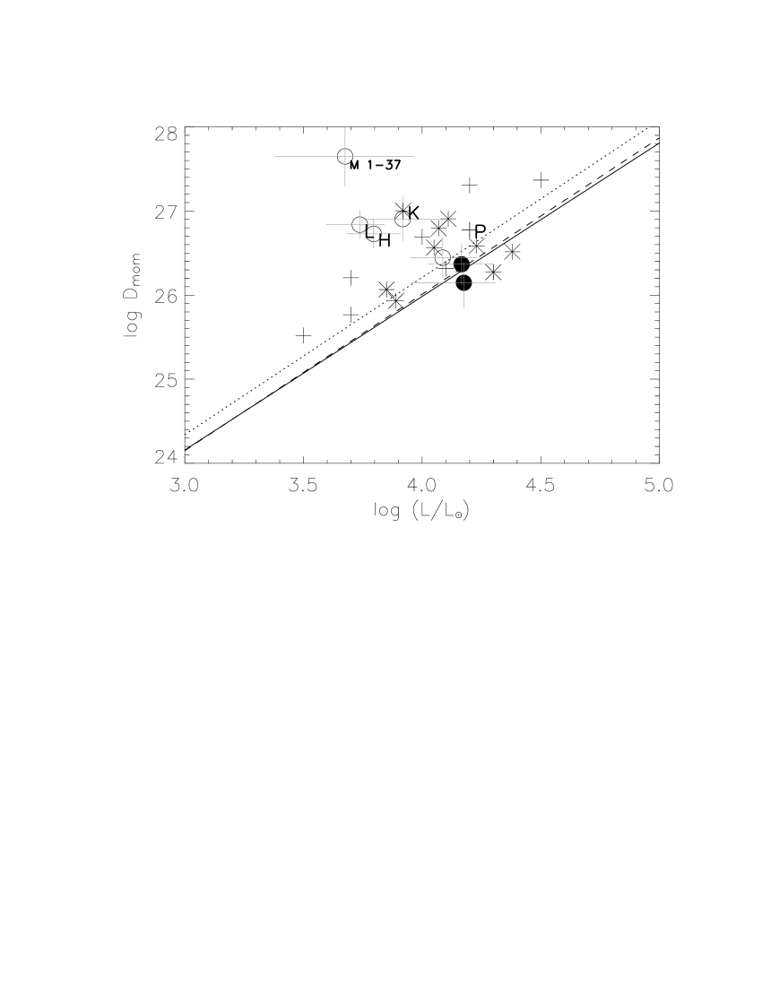
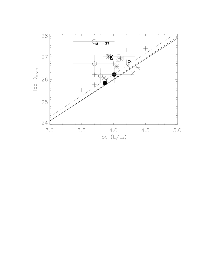
Figure 13: Modified wind-momentum rates, $D_{\rm mom}$, as a function of luminosity. Left: results from “Method 1”; right: results from “Method 2”. Circles correspond to the results for our sample (open: $f_{\rm cl}$ = 1, filled: $f_{\rm cl}\neq$ 1), asterisks to the results from Kudritzki et al. (2006) and pluses to the results from Pauldrach et al. (2004). The special symbols denote the various solutions for He 2$-$108, as in Figure 11. The solid line displays the theoretical prediction from Vink et al. (2000), and the dotted and dashed line the “observed” WLR for Galactic O-type supergiants and giants/dwarfs, respectively (from Markova et al. 2004). The object that deviates most from the predicted WLR is the most extreme object in our sample, M 1$-$37.

Comparing the luminosities shows a similar result. Except for M 1$-$37, the errors in $\log L_{\ast}$ derived by “Method 2” are twice as large as those from “Method 1”, whereas in the case of M 1$-$37 the errors are similar, due to the extremely large uncertainties in $\log g$ affecting the corresponding stellar radius derived by “Method 1”.

Concentrating on the parameters themselves (mass and radius), Figure 12 shows that for most of the objects the derived values agree within the error bars, but that the specific values can be quite different. Notably, the masses of three bulge-objects as derived from “Method 2” would be extremely low, whereas both solutions for He 2$-$108 result in implausibly high masses. Again, this is the outcome of the quadratic influence of a highly insecure stellar radius.

4.2.2 Distances

Provided that our atmospheric models do not contain intrinsic errors and that the evolutionary tracks of the central stars are generally applicable to all objects of this group, the uncertainties in the spectroscopic distances are dominated by the errors in the extinction towards the central stars (plus the error in $V$ for M 2$-$33). Remember that the derived masses are very accurate in this case, and that the errors in stellar radius result from a fairly small error propagation since $R_{\ast}\propto\sqrt{M_{\ast}/g}$. In order to account for the unclear situation regarding reddening, we assumed rather large errors for $A_{V\,{\rm optical}}$ (standard reddening) and $A_{V\,{\rm radio}}$ ($R_{V}\approx 2.6$), namely the mean difference between both quantities for our sample ($\Delta A_{V}=\pm 0.6$ mag), whereas for the “mean” extinction, $A_{V\,{\rm mean}}$, we assumed, because of the applied compromise, individual errors of $\Delta A_{V\,{\rm mean}}=\pm 0.5\leavevmode\nobreak\ (A_{V\,{\rm radio}}-A_{V\,{\rm optical}})$ which are roughly a factor of two smaller.

The resulting distances for $A_{V\,{\rm mean}}$ are displayed in Figure 12 (lower right panel), and those using either $A_{V\,{\rm optical}}$ or $A_{V\,{\rm radio}}$ are tabulated in Table 3. At first note that for the supposed bulge objects we derive distances in the range of $7.8\,\dots 11.5$ kpc when using the “mean” extinction, whereas for the alternative solutions $A_{V\,{\rm optical}}$ and $A_{V\,{\rm radio}}$ we derive distances that are smaller and larger, respectively.

Regarding the specific values, the distances derived by using $A_{V\,{\rm optical}}$ are best compatible with a bulge population. This becomes immediately clear if we assume that our sample is statistically distributed, and we calculate an (error-weighted) mean distance (leaving out M 1$-$37 since it has been placed inside the bulge, see Section 3.5.2). In this case, we obtain the values found in Table 4. Further consequences of these results are discussed in Section 5.

Table 4: Derived mean distances using different $A_{V}$ disregarding object M 1$-$37 (see text).

extinction	$A_{V\,{\rm mean}}$	$A_{V\,{\rm optical}}$	$A_{V\,{\rm radio}}$
mean distance (kpc)	10.7 $\pm$ 1.2	9.0 $\pm$ 1.6	12.2 $\pm$ 2.1

Both distances that we obtain for He 2$-$108 (low and high temperature solution) are fairly similar, and the differences with respect to the re-scaled distances from Méndez et al. (1992) and Kudritzki et al. (2006) (compare with the entry according to $A_{V\,{\rm mean}}$) are due to the different gravity resulting from our analysis and the applied centrifugal correction, which has been neglected previously. For this object, the influence of different extinction/reddening-laws is not as large as for the bulge objects, because the extinction itself is low.

4.3 Mass loss rates and wind momenta

Since the diagnostics used (H$\alpha$ and He ii $\lambda$4686) constrain the wind-strength parameter, $Q$ (or, even worse, only the product $Q\sqrt{f}_{\rm cl}$), also the mass-loss rates and the (modified) wind momentum rates depend on radius (and $v_{\rm\infty}$), via $\dot{M}=Q\leavevmode\nobreak\ (R_{\ast}\leavevmode\nobreak\ v_{\rm\infty})^{3/2}$ and $D_{\rm mom}=Q\leavevmode\nobreak\ R_{\ast}^{2}\leavevmode\nobreak\ v_{\rm\infty}^{5/2}$. Figure 12 (lower left panel) compares the latter quantities as resulting from “Method 1” and “2”. At least on the logarithmic scale, they are quite similar, though the errors from “Method 2” are larger, of course.

Figure 13 displays our results together with those derived from other investigations and theoretical predictions, in form of the wind-momentum luminosity diagram (left panel: “Method 1”; right panel: “Method 2”). Circles correspond to our investigation, denoted as open for objects with $f_{\rm cl}$ = 1, and filled for those two objects which show clear evidence for clumping.

The positions found for our objects scatter in a similar way around the “observed” WLR for Galactic O-type supergiants and giants/dwarfs (dotted/dashed, from Markova et al. 2004) and the corresponding theoretical predictions (solid, from Vink et al. 2000) as the results obtained by Kudritzki et al. (2006, asterisks) for a different sample, with He 2$-$108 in common. We also show the results from Pauldrach et al. (2004, crosses), obtained from a UV-analysis based on a consistent solution of the hydrodynamics.

Leaving aside the most extreme outlier, those two CSPN with clumping corrections lie close to but below the O-star WLR, one object is on the WLR and the other two well above. Since we are not able to exclude clumping corrections for the latter objects, it might be that they also follow the O-star trend. As already outlined by Kudritzki et al. (2006), however, a definite statement regarding the question of whether CSPN are a low luminosity extension of the O-star relation (as suggested by Pauldrach et al. 1988 and Kudritzki et al. 1997) or whether there is no such clear relation (see also Tinkler & Lamers 2002) is still not possible at the present stage.

There is one additional argument which might support the former hypothesis. If one claims that the CSPN indeed form such an extension, one obtains a certain constraint on their wind-strength parameter, $\log Q$: Rewritten in terms of this parameter, the WLR for a certain class of objects reads

$$\log D_{\rm mom} \approx x\log L+D,\qquad{\rm i.e.,}$$

$$\log Q+2\log R_{\ast}+\frac{5}{2}\log v_{\rm\infty} \approx 4\,x\log T_{\rm\kern-1.04996ptef\kern-0.35002ptf}+2\,x\log R_{\ast}+D^{\prime}$$

$$(v_{\rm\infty} \propto v_{\rm esc}=\sqrt{gR_{\ast}})$$

$$\log Q+(2-2\,x+\frac{5}{4})\log R_{\ast} \approx 4\,x\log T_{\rm\kern-1.04996ptef\kern-0.35002ptf}-\frac{5}{4}\log g+D^{\prime\prime},$$ (5)

with $x$ and $D$ the slope and offset of the specific WLR. If now the CSPN would follow such a WLR and were an extension of the O-star relation, this equation implies

$$(\log Q-0.5\log R_{\ast})_{\rm CSPN}=(\log Q-0.5\log R_{\ast})_{\rm O-stars}\,,$$ (6)

if we compare CSPN and O-stars of similar effective temperatures and gravities, using a typical slope of $1/x=0.53$ for the O-star WLR. In other words, the average wind-strengths of CSPN must be roughly 0.5 dex larger than the corresponding O-star values at same $T_{\rm\kern-1.04996ptef\kern-0.35002ptf}$ and $\log g$, if we adopt a typical difference of 1 dex in radii. But this is what we actually see in our spectra (cf. Section 3.5): Compared to O-supergiants of similar spectral type, all our sample stars show much more emission in H$\alpha$, immediately pointing to a higher $\log Q$. Indeed, the average value for our sample is $\log Q$ = $-$11.9, compared with typical (late) O-supergiant values in between $-$12.8 to $-$12.4.

Summarizing, a similar WLR implies that for CSPN one expects larger $Q$ (for smaller $R_{\ast}$ and $v_{\rm\infty}$), whereas, vice versa, the observed, strong H$\alpha$ emission might imply that the CSPN indeed lie on the O-star WLR. Alternatively, there is the possibility that the clumping properties of O-stars and CSPN differ significantly, with stronger clumping in CSPN.

5 Discussion

This project has produced a remarkable mixture of encouraging and alarming results. On the positive side, leaving aside M 1$-$37 with its unique spectrum and uncertain $\log g$, the four remaining bulge central stars turn out to have “Method 1” spectroscopic distances within $\pm 10$% to $\pm 15$% (depending on the extinction law) of their average distance, well within the expected uncertainties. The alarming fact is of course that their average distance, if we adopt the reddening corrections suggested by Stasinska et al. (1992), is a factor 1.5 larger than the currently accepted distance to the Galactic bulge. This allows the following possible interpretations:

• If the reddening corrections based on a low $R_{V}$ and radio-H$\beta$ extinctions are correct, then the combination of our model atmospheres plus standard post-AGB evolutionary tracks gives systematically too large spectroscopic distances, despite their excellent internal agreement.

• If the standard reddening law is valid, and using $C_{\rm opt}$, then our “Method 1” spectroscopic distances give the right distance to the Galactic bulge to within 13%, which would have to be considered a successful test; but then we need to find a reason for the observed systematic difference between the optical and radio-H$\beta$ extinctions.

In the present situation we do not feel that we have enough information to decide between (1) and (2). Our referee, A. Zijlstra, has pointed out that our sample objects have (by bad luck) relatively poorly known radio fluxes. Most come from very old radio data, obtained at the very start of the VLA, and we cannot be as confident of these as we are of more recent observations. Only He 2$-$260 can be considered as reliable; the others need confirmation.

The analysis of our comparison object from the “solar neighborhood”, He 2$-$108, reveals a prototypical CSPN mass, of about $0.6M_{\odot}$ (both for the low and high $T_{\rm\kern-1.04996ptef\kern-0.35002ptf}$ solution) if “Method 1” is followed. This is in agreement with the $0.67M_{\odot}$ derived by Méndez et al. (1992) and the recent value of $0.63M_{\odot}$ by Kudritzki et al. (2006). The higher masses derived using “Method 2”, however, lacks any significance (except for the fact that it overlaps within the error bars with our “Method 1”-mass), due to its highly uncertain distance (adopted from similar analyses) and the large error propagation of this quantity. Recently, Napiwotzki (2006) has claimed, using an analysis of kinematical parameters based on simulated Galactic orbits, i.e., by means of a completely different approach, that a low mass similar to our “Method 1” result would be more compatible with the kinematical parameters one would expect from a member of the thin-disk population.

On the other hand, Pauldrach et al. (2004) derived a significantly larger mass of $1.33M_{\odot}$ for this object. In contrast to our approach, they have solved the hydrodynamical equations in a self-consistent way, and compared the corresponding, synthetic UV spectra with observations. $T_{\rm\kern-1.04996ptef\kern-0.35002ptf}$ then follows from the observed ionization equilibrium, whereas mass and radius are uniquely constrained from the terminal velocity (being proportional to the photospheric escape velocity, $\propto(M_{\ast}/R_{\ast})^{1/2}$, and mass-loss rate (depending on luminosity, i.e., again on stellar radius). Note that both wind parameters are clearly “visible” in the UV-lines.

Ideally, the results of optical and UV spectroscopy should be similar. By comparing the derived effective temperatures and gravities for our high $T_{\rm\kern-1.04996ptef\kern-0.35002ptf}$ solution (Fig. 11, ‘H’ vs. ‘P’), at least for these parameters this is indeed the case (i.e., the ratios $M_{\ast}/R_{\ast}^{2}$ do agree). Thus, the difference in mass is due to a different radius (implying different ratios $M_{\ast}/R_{\ast}$) which in the case of Pauldrach et al. (2004) results from hydrodynamical considerations, whereas here we have derived the mass directly from evolutionary tracks.

A solution of this discrepancy cannot yet been provided, but will be commented on in the following. At first, let us give a few additional remarks concerning PN distances. In the same publication as just referred to, Pauldrach et al. (2004) presented a comparison between spectroscopic and other PN distance determinations, which will not be repeated here except to comment on the fact that one of the very few cases of a clear discrepancy (Hipparcos parallax of PHL 932) has been resolved in favor of the spectroscopic distance. Harris et al. (2007) reports new trigonometric parallaxes for several central stars, pointing out that the Hipparcos parallax of PHL 932 is wrong. The new geometric distance of PHL 932 is 300 pc, in perfect agreement with the spectroscopic distance we obtain if we assume a stellar mass of 0.3 $M_{\odot}$ and the following atmospheric parameters: $T_{\rm\kern-1.04996ptef\kern-0.35002ptf}=36\,000$ K and $\log g=5.7$, which are the averages from two independent spectroscopic studies (Méndez et al. 1988a and Napiwotzki 1999). Clearly the Harris geometric distance confirms the small stellar mass and proves definitely that PHL 932 cannot be a post-AGB star (Méndez et al., 1988a). So here we have a case where the model atmospheres pass the test. Harris et al. (2007) also shows agreement, within the uncertainties, between his parallaxes and spectroscopic distances for several PN, mostly from Napiwotzki (1999).

Of course we must add that those central stars with trigonometric parallaxes are high-gravity stars with no wind features; so this agreement is not a confirmation of the wind models. The same comment applies to the central star of K 648, the PN in the globular cluster M 15, whose spectroscopic distance is in excellent agreement with the cluster distance (McCarthy et al., 1997). Let us argue in the following way: if the combination of post-AGB theory and windless model atmospheres gives good distances (as indicated by the high-gravity stars and K 648) and the combination of post-AGB theory and wind models fails systematically, then it would be easy to conclude that the wind models must be wrong. But this is not the case – evidence for such systematical failures have not been found so far, and it should be noted that our Galactic bulge sample includes central stars with weak and strong winds, yet all their “Method 1” spectroscopic distances agree, with no differences that could be attributed to wind strength effects. Alternatively, we have the possibility that another group of CSPN with winds exists (e.g., some objects from the sample analyzed by Pauldrach et al. 2004), which follow a different evolutionary path and for which the standard CSPN tracks do not apply. A further indication of such a possible qualitative difference is the fact that Kudritzki et al. (2006), using a similar method as in this paper, also based on the standard evolutionary tracks, found higher masses (around $0.74\,M_{\odot}$) for the same sample of objects as analyzed by Pauldrach et al. (2004), whereas the mean mass of the CSPN in our current sample is around $0.68\,M_{\odot}$.

In summary, the combination of excellent internal agreement (and some additional supporting evidence) plus the extinction problem leads us to conclude that our Galactic bulge distance test is undecided.

We can see two ways of trying to force a decision:

• a careful, multi-wavelength redetermination of the interstellar extinction toward the bulge PN we have studied,

• enlarge the sample of bulge central stars, trying to get high-quality, high-resolution spectrograms with minimum nebular contamination.

Alternatively, as already emphasized in the introduction, post-AGB tracks and model atmospheres could be independently tested as soon as medium-resolution spectroscopy of CSPN in the Magellanic Clouds, with efficient nebular light subtraction, becomes feasible; the advantage being the small amount of reddening in that direction.

6 Summary and conclusions

We have selected a small sample of PN central stars in the Galactic bulge and obtained high-resolution spectrograms with the Keck HIRES spectrograph. We present spectral classification of these central stars and we model their optical spectral features (including wind effects) using a state of the art non-LTE, spherically symmetric model atmosphere code that includes the effects of line blocking/blanketing and wind clumping. We obtain effective temperatures, surface gravities, wind parameters and He and Si abundances. With one exception, He and Si abundances are normal for H-rich central stars. The exception is M 1$-$37, a central star with spectacular P Cygni profiles indicative of a very dense wind, He-rich, and with an apparently very high Si abundance, 28 times solar, unexplained for the moment. This star also shows strong unidentified emissions at 4485 and 4504 Å, which we have refrained from identifying with Silicon.

Armed with the stellar atmospheric parameters we then calculate other parameters not directly derivable from our analysis, using two methods. “Method 1” uses post-AGB evolutionary tracks to read masses, from which stellar radii, luminosities, mass loss rates and spectroscopic distances follow. “Method 2” assumes the distance to the Galactic bulge and derives stellar radii and other quantities; this method turns out to be very uncertain because of the strong dependence of mass on stellar radius, which is itself not well determined.

If we focus our attention on the results of “Method 1”, the most remarkable conclusion regards the internal agreement of the spectroscopic distances of at least four bulge central stars within our sample (leaving aside the extreme object M 1$-$37 with its ill-defined gravity): all of them are quite the same to within $\pm 10$% to $\pm 15$% (depending on the extinction law) of their average distance. This result is well within the expected uncertainties. There is a problem, however: the average distance to the Galactic bulge is strongly dependent on the adopted reddening correction, to such an extent that we cannot decide if “Method 1” passes the consistency test for our sample (if we adopt the most recently derived reddening corrections, the average distance turns out to be a factor 1.5 larger than the currently accepted distance to the Galactic bulge). Additional studies of extinction for the PN in our sample will be necessary, and it would be good to increase the size of the bulge CSPN sample subject to this kind of analysis, while we wait for a chance to repeat this kind of study in the Magellanic Clouds, which are almost free of the extinction problem.