Further Evidence for an Elliptical Instability in Rotating Fluid Bars and Ellipsoidal Stars

Abstract

Using a three-dimensional nonlinear hydrodynamic code, we examine the dynamical stability of more than twenty self-gravitating, compressible, ellipsoidal fluid configurations that initially have the same velocity structure as Riemann S-type ellipsoids. Our focus is on “adjoint” configurations, in which internal fluid motions dominate over the collective spin of the ellipsoidal figure; Dedekind-like configurations are among this group. We find that, although some models are stable and some are moderately unstable, the majority are violently unstable toward the development of $m=1$, $m=3$, and higher-order azimuthal distortions that destroy the coherent, $m=2$ bar-like structure of the initial ellipsoidal configuration on a dynamical time scale.

The parameter regime over which our models are found to be unstable generally corresponds with the regime over which incompressible Riemann S-type ellipsoids have been found to be susceptible to an elliptical strain instability (Lebovitz & Lifschitz, 1996). We therefore suspect that an elliptical instability is responsible for the destruction of our compressible analogs of Riemann ellipsoids. The existence of the elliptical instability raises concerns regarding the final fate of neutron stars that encounter the secular bar-mode instability and regarding the spectrum of gravitational waves that will be radiated from such systems.

1 Introduction

In a previous paper (Ou, 2006, hereafter paper I), we introduced a new self-consistent-field technique that is capable of constructing three-dimensional (3D) models of incompressible Riemann S-type ellipsoids and compressible triaxial configurations that share the same velocity fields as those of Riemann S-type ellipsoids. These compressible triaxial configurations represent fairly good quasi-equilibrium states and can be used to examine the dynamical stability of Riemann S-type ellipsoids in the nonlinear regime. With this in mind, a subset of our compressible models have been evolved in a 3D hydrodynamics code (Motl, Tohline, & Frank, 2002) for $20-40$ dynamical times to test their dynamical stability. In this paper, we present results from these hydrodynamic simulations.

Before going into the details of our simulations, it is worthwhile spending some time reviewing previous studies of the stability properties of Riemann S-type ellipsoids. Chandrasekhar and Lebovitz carried out a vigorous analysis of the stability of Riemann S-type ellipsoids with respect to second and third order harmonics (these results are summarized in Chandrasekhar (1969)). Some configurations, including both rigidly-rotating Jacobi and stationary Dedekind sequences, were found to be subject to a pear-mode (azimuthal mode number $m=3$) instability beyond a certain point while proceeding away from the axisymmetric Maclaurin spheroid sequence. Part of the Jacobi and Dedekind sequences were also found to be unstable to a dumbbell-shaped (azimuthal mode number $m=4$) mode; this has provided some theoretical foundation for the fission theory of the formation of binary stars (Durisen & Tohline, 1985; Lebovitz, 1987; Tohline, 2002). These studies have assumed that the evolution of a rotating gas cloud toward the bifurcation points of the $m=3$ pear-mode or $m=4$ dumbbell-mode proceeds in a quasi-stationary manner and on a time scale that is fairly long compared to the dynamical time scale.

However, more recent linear stability studies (Lebovitz & Lifschitz, 1996; Lebovitz & Saldanha, 1999) have revealed a new elliptical strain instability in Riemann S-type ellipsoids that is associated with the noncircular fluid streamlines that describe the internal motion of these configurations. According to these studies, a fairly large fraction of all rotating ellipsoids appear to be susceptible to the development of this elliptical instability. It has a growth rate that is slow compared to the rotation rate but is nevertheless dynamical. The fastest growth rates are found among the adjoint configurations, in which the internal motion dominates over the collective pattern motion of the rotating bar. This elliptical instability was first discovered and studied by Pierrehumber (1986) and Bayly (1986) in the context of two-dimensional (2D), incompressible fluid flows. Goodman (1993), Lubow, Pringle & Kerswell (1993), and Ryu & Goodman (1994) extended it to astrophysics to study tidally distorted accretion disks. They found that the instability is three-dimensional (depends on the vertical dimension) and approximately incompressible, and that it might also give birth to $m=1$ internal waves in the absence of viscosity. It is subsequent to this work on accretion disks that Lebovitz & Lifschitz (1996) conducted their study of Riemann S-type ellipsoids, for which elliptical flows are generic.

The discovery of an elliptical strain instability in rotating ellipsoidal (bar-like) structures brings into question (Lebovitz & Lifschitz, 1996) whether the paradigm for evolution of a secularly unstable star driven by gravitational-radiation reaction (GRR) forces is viable. According to this paradigm (Chandrasekhar, 1970; Detweiler & Lindblom, 1977; Lai & Shapiro, 1995), such a star – in the form of a Riemann S-type ellipsoid – would evolve on a secular time scale toward the Dedekind sequence (for which the pattern frequency of the bar-mode $\omega=0$), at which point the evolution would stop because the gravitational field no longer exhibits a time-varying quadrupole moment. The analysis of Lebovitz & Lifschitz (1996) shows that the parameter space occupied by the elliptical instability encompasses most of the Dedekind sequence. Because the elliptical instability develops on a dynamical time scale, it might prevent a GRR-driven figure from proceeding further to the Dedekind sequence, especially if the elliptical instability develops into the nonlinear regime. Because the results presented by Lebovitz & Lifschitz (1996) are based on linear analysis, they were not sure what the nonlinear outcome of the elliptical instability would be.

In a recent nonlinear study of the development of the secular bar-mode instability by Ou, Tohline, & Lindblom (2004), an initially uniformly rotating neutron star was driven by GRR forces into a differentially rotating bar-like configuration that had a very low pattern frequency. This bar-like configuration appeared to be a compressible analogue of an adjoint configuration among the Riemann S-type ellipsoids. However, the coherent bar-like structure was destroyed very quickly by the nonlinear development of an unexpected high-order instability that generated “turbulence” throughout the internal structure of the bar. Ou, Tohline, & Lindblom (2004) suggested that this turbulent-like instability was related to the elliptical instability, but no definite conclusion could be drawn because only one model was studied. It was impractical to pursue a full investigation across the entire parameter space of possible ellipsoidal models because, at the time, the generation of one single equilibrium bar-like model was computationally expensive; the construction of even one equilibrium ellipsoidal model required following the GRR-driven evolution of an initially axisymmetric model, which takes a very long time even with an artificially enhanced GRR force (Ou, Tohline, & Lindblom, 2004; Shibata & Karino, 2004).

With the new self-consistent-field technique introduced in Paper I, we have been able to quickly build a large number of nearly incompressible, quasi-equilibrium triaxial models. These compressible models contain the same internal velocity flow-fields as incompressible Riemann ellipsoids. And although they are not exact steady-state configurations, these models provide reasonably good initial states for a study of the elliptical instability because the elliptical instability develops on a dynamical time scale. In what follows, we present hydrodynamic simulations of a variety of these nearly incompressible, rotating bar-like models to test their dynamical stability. We find that a significant fraction are unstable to what appears to be the elliptical instability. We introduce our initial models and analysis method in §2; we present results from hydrodynamic evolutions for different configurations in §3; and in §4, we conclude and discuss issues relevant to the evolutionary path of secularly unstable neutron stars.

2 Initial Models and Methods

2.1 Initial Models

We follow the notation defined in Paper I, where $a$, $b$, and $c$ are the three principal semiaxes of an ellipsoid and $c$ is the rotation axis. In a frame of reference whose origin coincides with the center of the ellipsoid and that is rotating with the pattern frequency of the ellipsoid, $\omega$, the velocity field of a Riemann S-type ellipsoid takes the form,

$$\vec{v}=\lambda(ay/b,-bx/a,0)\,,$$ (1)

where $\lambda$ is a constant that determines the degree of internal motion of the fluid. This velocity field is designed so that velocity vectors are everywhere tangent to a set of self-similar concentric ellipses. (In the uniform-density, incompressible Riemann configurations, these concentric ellipses also identify equipotential contours.) When $|\omega|>|\lambda|$, a model is said to be a “direct” model, in which the figure rotation dominates over internal motions. Conversely, when $|\omega|<|\lambda|$, the configuration represents an “adjoint” model, in which the internal fluid motion dominates over the figure rotation.

In Paper I, we constructed a variety of compressible models that have the same velocity field as is found in incompressible Riemann S-type ellipsoids, that is, with the velocity field defined by Eq. (1). These models satisfied the steady-state Euler’s equation exactly, but only satisfied the steady-state continuity equation approximately. However, as discussed in Paper I, it was found that the deviation from the steady-state continuity equation was small for models that obeyed a relatively stiff equation of state (EOS). For our present study, we have used the same self-consistent-field technique described in Paper I to construct more than forty quasi-equilibrium, compressible analogues of Riemann S-type ellipsoids to serve as initial states for a series of hydrodynamic simulations. The models were constructed using two different EOS ($n=0.5$ and $n=1$ polytropes), with a variety of initial axis ratios – Figure 14 displays the range of selected ($b/a$, $c/a$) pairs – and, for a given set of axes, both “direct” and “adjoint” configurations were constructed. This set of models was selected to cover a reasonably large fraction of the parameter space that was investigated by Lebovitz & Lifschitz (1996), keeping in mind that their linear analysis was confined to incompressible figures.

The stability of roughly twenty-five of these initial models was examined using a 3D hydrodynamic code, as explained below. We focused on analyzing the stability of adjoint models with an $n=0.5$ polytropic EOS, but several direct models with an $n=0.5$ EOS and one adjoint model with an $n=1$ EOS were included in the mix. For the sake of brevity, only the results of six model evolutions are presented in detail in §3. Table 1 lists the key parameters for these six representative models. In addition to the name that has been assigned to each model and the values of five parameters that already have been defined ($n$, $b/a$, $c/a$, $\omega$, $\lambda$), Table 1 specifies each initial model’s ratio of rotational to gravitational potential energy $T/|W|$, total angular momentum $J_{\mathrm{tot}}$, mean density $\rho_{\mathrm{mean}}$ , and the ratio of the pattern period $T_{p}\equiv 2\pi/\omega$ to the dynamical time $T_{\mathrm{dyn}}\equiv[\pi G\rho_{\mathrm{mean}}]^{-1/2}$. The measured growth rates $T_{1}$ and $T_{3}$ of unstable modes with azimuthal mode numbers $m=1$ and $m=3$ are also tabulated (see §3 for further elaboration). Dimensional quantities are in the hydro code unit for which the gravitational constant $G$, the central density $\rho_{c}$, and the cylindrical radius of the entire grids $\varpi_{grid}$ are all set to unity. If the first letter in a model’s name is D, the model is a “direct” configuration, whereas an A denotes an “adjoint” configuration. Among this group of six models, we note that only model A067 has a polytropic index $n=1$; the other models all have $n=0.5$.

Table 1: Parameters of selected initial models

model	$n$	$b/a$	$c/a$	$\omega$	$\lambda$	$T/|W|$	$J_{\mathrm{tot}}$	$\rho_{\mathrm{mean}}$	$T_{p}/T_{\mathrm{dyn}}$	$T_{1}/T_{\mathrm{dyn}}$	$T_{3}/T_{\mathrm{dyn}}$
D105	0.5	0.59	0.487	0.911	0.114	0.105	0.00809	0.526	1.4	-	-
D080	0.5	0.49	0.487	0.885	0.230	0.080	0.00497	0.529	1.5	-	-
A010	0.5	0.74	0.821	-0.610	-0.875	0.010	7.24e-3	0.543	2.1	-	-
A067	1.0	0.90	0.692	-0.168	-0.796	0.067	0.0087	0.280	5.6	-	-
A134	0.5	0.74	0.487	-8.1e-3	-0.911	0.134	0.0133	0.519	158	3.3	3.4
A100	0.5	0.59	0.487	-0.114	-0.911	0.100	7.21e-3	0.526	11	1.4	1.3

2.2 Methods

In order to examine their relative stability, each model was evolved on a cylindrical coordinate mesh using the 3D, Newtonian, finite-volume computational fluid dynamics technique described in detail by Motl, Tohline, & Frank (2002). In each simulation, the adopted grid resolution was $66\times 102\times 128$ in the $\varpi$ (cylindrical radius), $z$ (vertical), and $\phi$ (azimuthal) directions, respectively.

We monitor the time-evolution of the general structure of each model by measuring the Fourier amplitude of various “modes” having azimuthal quantum numbers $m$ in the following fashion: At each instance of time, the azimuthal density distribution in a ring of fixed $R$ and $z$ can be decomposed into a series of azimuthal Fourier components via the relation,

$$\rho(R,z,\phi)=\sum\limits_{m=-\infty}^{+\infty}C_{m}(R,z)e^{im\phi}\,,$$ (2)

where the complex amplitudes $C_{m}$ are defined by the expression,

$$C_{m}(R,z)=\frac{1}{2\pi}\int_{0}^{2\pi}\rho(R,z,\phi)e^{-im\phi}d\phi\,.$$ (3)

In our simulations, the time-dependent behavior of the magnitude of this coefficient, $|C_{m}|$, is monitored at a variety of $(R,z)$ locations to measure the growth-rate of various modes. The time-varying amplitudes shown in our figures, below, are averages of $|C_{m}|$ over the entire volume.

Although this diagnostic tool permits us to study the behavior of structure having a wide variety of $m$ values, in practice we have focused our attention on the lowest order modes for this study. For example, a trace of the time-evolution of $|C_{2}|$ lets us monitor the overall ellipticity of each model. The $m=2$ mode should dominate initially because of each model’s initial bar-like structure. If this amplitude remains at a fairly constant level in a given simulation, we conclude that the configuration is stable; otherwise, it is unstable. In practice, we have found that when the $m=2$ amplitude drops significantly in a model, that model simultaneously displays growth of other azimuthal modes.

In their analysis of the elliptical instability, Lebovitz & Lifschitz (1996) generally found that the unstable mode with the fastest growth rate was the $m=3$ mode. In their study, the $m=1$ mode was not discussed because, in incompressible configurations, an $m=1$ mode normally refers to a translation of the center of mass of the configuration. However, in the study of an elliptical instability in tidally distorted accretion disks by Goodman (1993) and Lubow, Pringle & Kerswell (1993), it was found that an eccentric $m=1$ mode may be important. Further investigation shows that the instability has some dependence on the third (vertical) dimension, because it disappeared in 2D simulations (Ryu & Goodman, 1994). With these results in mind, we have focused our attention on the development of the $m=1$ and $3$ modes in our 3D ellipsoidal model evolutions.

3 Results From Hydrodynamic Simulations

We present our results from hydrodynamic evolutions for direct and adjoint configurations in the next two subsections, respectively.

3.1 Results For Direct Configurations

In this subsection, we present results from two direct configurations, models D105 and D080, which were evolved for about 24 $T_{\mathrm{dyn}}$ and 17 $T_{\mathrm{dyn}}$, respectively. Figure 1 shows snapshots in time of equatorial-plane iso-density contours and the inertial-frame velocity field for model D105. (In the online version of this paper, the figure caption includes a link to an MPEG movie showing the entire evolution of this model.) This model is stable; the coherent bar-like structure and elliptical flows are well maintained throughout the 24 $T_{\mathrm{dyn}}$ followed by our simulation. The time-varying Fourier mode amplitudes displayed in Figure 2 show that the $m=2$ bar-mode remains the dominant mode throughout this evolution, with an amplitude that remains approximately three orders of magnitude higher than those of the $m=1$ and $3$ modes. Although the $m=4$ mode has a larger amplitude than the odd modes, the fact that its behavior follows that of the $m=2$ mode suggests that it is a harmonic of the $m=2$ mode and that there is no independent $m=4$ mode.

Although we have categorized model D105 as stable, a slow decay of the bar-mode amplitude is evident in Figure 2. Because other modes, including the $\mathrm{m}=1$ and $3$ modes, do not grow throughout the evolution, this slow decay of the bar-mode probably results from the small violation of the steady-state continuity equation in our initial model configuration. (This, in turn, results from the fact that the 3D iso-density surfaces in our compressible models deviate from self-similar ellipses or homeoidal shells; see Paper I for a more detailed discussion.) Small violations in the surface layers cause very low density material to be shed outward from both ends of the object and form two low density spiral waves (see the panel labeled $t=5$ in Figure 1). Because this material carries relatively high specific angular momentum, the overall system loses angular momentum, but only on a very long time scale. We suspect that this is the major cause of the gradual decay of the $m=2$ bar-mode in this model evolution.

Figure 3 shows a similar Fourier mode analysis for model D080. Again, the ${m}=2$ bar-mode dominates the entire evolution and shows a slow decay; amplitudes of the odd azimuthal modes remain at roughly constant “noise” levels.

The results from the evolution of these two direct configurations suggest that, although our initial model configurations do not satisfy the steady-state continuity equation exactly, the models are still fairly good quasi-equilibrium states. In both cases, the coherent bar-like structures were well maintained through $\sim 20$ $T_{\mathrm{dyn}}$. Hence, we are confident that initial models generated by the technique described in Paper I can be used to study the dynamical stability of compressible Riemann S-type ellipsoids. Furthermore, the fact that the elliptical instability sets in on a dynamical time scale will allow us to use these models to detect the elliptical instability, if it exists.

According to Lebovitz & Lifschitz (1996, see their Figure 2 for a summary of their analysis of direct configurations), the elliptical instability only arises in a small portion of the parameter space that is occupied by direct configurations, and its growth rate is relatively slow there. This makes it relatively difficult for our current study to identify the exact parameter-space boundaries between stable and unstable direct configurations. Furthermore, the method described in Paper I can only be used to construct compressible models having axis ratios $b/a\gtrsim 0.5$, whereas most of the domain that we expect to be effected by the elliptical instability in direct configurations has $b/a<0.5$. This also makes direct configurations unsuitable for identifying the existence of the elliptical instability.

Therefore, we have chosen to focus our study on an analysis of adjoint configurations where the domain of the instability is much wider, according to Lebovitz & Lifschitz (1996, see especially their Figure 3a, which is reproduced here as Figure 13). More importantly, the growth rate of the instability is expected to be faster in adjoint configurations. This helps us to conduct such a survey with a limited evolution time that is allowed by our current computational resources. In the next subsection, we present simulations of adjoint configurations, which indeed reveal the development of turbulence-like flows that we suspect are associated with the elliptical instability.

Figure 1: Equatorial-plane iso-density contours and velocity fields in the inertial frame for model D105. Density contours correspond to $\rho/\rho_{\mathrm{max}}=0.01,0.1,0.5$, and $0.8$ from the outermost to the innermost shell, and time is given in units of $T_{\mathrm{dyn}}$. The pattern rotation of the overall ellipsoidal configuration and the internal fluid motion are both prograde (counterclockwise) in this “direct” model configuration. An accompanying MPEG movie shows the entire evolution of this model, through $t\approx 24~{}T_{\mathrm{dyn}}$; 3D, rather than 2D, iso-density contours are shown in the movie without the accompanying flow field.

Figure 2: Time-evolution of the amplitudes $|C_{m}|$ of the $m=1,2,3,$ and 4 modes for model D105. The amplitudes of the $m=2$ and 4 modes decay gradually; the $m=1$ and 3 modes remain at a fairly constant, low-amplitude level, which suggests that this “direct” model is stable against the elliptical instability.

Figure 3: The same as Figure 2, but for model D080. This “direct” model also appears to be stable against the elliptical instability.

3.2 Results of Adjoint Configurations and Existence of a Turbulent-like Instability

In this subsection, we present results from 3D hydrodynamic evolutions of the four adjoint configurations listed in Table 1. In light of previous studies (Goodman, 1993; Lebovitz & Lifschitz, 1996), it is expected that the $m=1$ and $3$ modes will be the fastest growing modes, if an elliptical instability sets in. Therefore, rapid growth of these two modes can serve as a compass pointing to the elliptical instability. With this in mind, in the analysis below we will categorize our results based on the behavior of these two modes. Based on the final outcome and behavior of the $m=1$ and $3$ modes, evolutions of our initially quasi-equilibrium compressible adjoint configurations can be divided into three categories: stable models, moderately unstable models, and violently unstable models.

The first category — stable models — consists of evolutions in which the internal elliptical flow remains stable. One evolution in this family is model A010, with $b/a=0.74$. Note from the information in Table 1 that this model has a somewhat prolate structure with $c>b$. Figure 4 shows 2D, equatorial-plane iso-density contours of this model at four different times. (The figure caption in the online version includes a link to an MPEG movie showing the entire evolution of this model.) The ellipsoidal shape is well preserved, at least up through the end of our simulation $\sim 26~{}T_{\mathrm{dyn}}$, and the internal elliptical flow pattern remains stable. As suggested by the Fourier mode analysis shown in Figure 5, the $m=2$ bar-mode dominates throughout the entire evolution. There is no indication that the $m=1$ and $3$ modes are growing; their amplitudes remain fairly constant at “noise” level throughout the evolution. Figures 6 and 7 show similar plots for another stable model, namely, model A067 with $b/a=0.90$. This model was perturbed with an initial low-amplitude $m=3$ perturbation, but its bar-like structure remains stable during the evolution. We note that the bar-mode appears to undergo a low-amplitude oscillation. As we have discussed in Paper I, initially small deviations from the steady-state continuity equation can generate surface waves in adjoint models. The oscillations observed here in the amplitude of the $m=2$ bar-mode is indeed a reflection of these low-amplitude surface waves traveling along the elliptical surface. The initial violation of the steady-state continuity equation is larger in models with a softer EOS (see Paper I). It is therefore not surprising that oscillations of the bar-mode amplitude in model A067 are somewhat larger than in other models because model A067 was constructed using a relatively soft ($n=1$ polytropic) EOS.

The second category of adjoint evolutions consists of configurations that are moderately unstable. In these models, the elliptical flow appears to remain stable as judged by the behavior of the $m=2$ Fourier mode. However, the $m=1$ and $3$ modes are observed to grow on a long time scale. Model A134 with $b/a=0.74$ belongs to this family. Figure 8 shows 2D iso-density contours of this model in the equatorial plane at different evolutionary times. (An MPEG movie showing part of the evolution of this model is available in the figure caption of the online version.) We note that this model has an almost vanishingly small bar pattern frequency, $\omega=-0.0081$, so it is very nearly a Dedekind-like object; as seen in Figure 8, the bar-like pattern shifts retrograde (clockwise) through only $\approx\pi/4$ radians over $15~{}T_{\mathrm{dyn}}$! Through this initial $\sim 15~{}T_{\mathrm{dyn}}$, the coherent ellipsoidal structure and elliptical flow pattern remain stable. However, as revealed by the Fourier mode analysis in Figure 9, at later times the ${m}=1$ and $3$ modes both exhibit exponential growth, albeit at a very slow growth rate. We note that the amplitudes of these odd modes appear to be tied to each other; even their individual growth rates are almost the same. (As recorded in Table 1, the e-folding time for these odd modes are $T_{1}=3.3T_{\mathrm{dyn}}$, and $T_{3}=3.4T_{\mathrm{dyn}}$.) This suggests that the mechanism that is responsible for driving these modes is probably the same. Their amplitudes do not exceed that of the $m=2$ mode at the end of this simulation. Hence, we have identified this model as being moderately unstable. Across the parameter space of our investigation (see, for example, Figure 14), models belonging to this category can be regarded as a transition from stable to violently unstable models.

The third category consists of models that are violently unstable to an instability that leads to apparently turbulent flow throughout the configuration. The $m=2$ bar-mode is quickly destroyed in a few dynamical times; simultaneously, both the $m=1$ and $3$ modes exhibit extremely fast exponential growth. One of the most unstable models in our investigation is A100 with $b/a=0.59$. The time-evolution of equatorial-plane iso-density contours of this model is shown in Figure 10. (The entire evolution is shown in a MPEG movie in the figure caption of this plot in the online version of this paper.) The initial ellipsoidal structure exists for only $\sim 3T_{\mathrm{dyn}}$, then it is suddenly destroyed by some type of “turbulent” instability. After the bar-like structure is destroyed, the whole configuration settles into an entirely turbulent state, exhibiting small-scale vortices and eddies. The Fourier mode analysis shown in Figure 11 looks distinctly different from all previous mode plots: the $m=2$ mode decays very quickly in parallel with rapidly growing ${m}=1$ and $3$ modes, which finally surpass the ${m}=2$ mode in amplitude. These distinct features suggest that the initially ellipsoidal structure of model A100 was destroyed by a process that is entirely different from the gradual decay of the bar-mode amplitude seen in our models that have been categorized as stable. As in model A134, the growth time for both the $m=1$ and 3 modes are very close to each other (as recorded in Table 1, $T_{1}=1.4T_{\mathrm{dyn}}$ and $T_{3}=1.3T_{\mathrm{dyn}}$), but they ultimately saturated at different levels. We evolved model A100 for a long time ($\sim 50T_{\mathrm{dyn}}$) until the system reached a new, nearly axisymmetric state.

The turbulent behavior of model A100 is very similar to the outcome of an instability that arose during the late evolution of the GRR-driven neutron star from a previous study (Ou, Tohline, & Lindblom, 2004). In an effort to compare this earlier simulation result with our present one, we have plotted in Figure 12 a power spectrum of the various azimuthal modes for model A100 at time $t=0$ and $t=45T_{\mathrm{dyn}}$ in the evolution. This power spectrum looks surprisingly similar to the power spectrum that was generated by Ou, Tohline, & Lindblom (2004) late in their model’s evolution. The spectrum is dominated by even modes in the beginning as a result of the ellipsoidal (bar-like) structure; whereas a turbulence-like power law distribution dominates at late times, after the energy initially stored in the $m=2$ bar-mode has cascaded into all other Fourier modes. This strongly suggests that the violent instability seen in our present study is the same instability that arose in the Ou, Tohline, & Lindblom (2004) investigation. Because this turbulence-like instability has arisen in two quite different contexts — Ou, Tohline, & Lindblom (2004) discovered it while studying the non-linear evolution of an initially axisymmetric star that was driven to a bar-like configuration by GRR forces, whereas we have discovered it during purely hydrodynamic evolutions of compressible triaxial models that have been purposely constructed to resemble adjoint configurations of Riemann S-type ellipsoids — it seems likely that the instability is generic to adjoint configurations.

In an effort to understand whether or not this instability occupies the same regions of parameter space as the elliptical instability studied by Lebovitz & Lifschitz (1996), our hydrodynamic investigation has included models that cover as much parameter space as possible. In Figure 14, we have mapped the results from 20 of our adjoint model evolutions onto the $(b/a,c/a)$ plane. (For the sake of brevity, a detailed discussion of only 6 of these model evolutions has been presented, above.) Models found to be violently unstable are marked by asterisks, stable models are marked by diamonds, and moderately unstable models are marked by plus signs. This figure should be compared with Figure 3a from Lebovitz & Lifschitz (1996) – reproduced here as Figure 13 – which shows the instability domain occupied by the $m=3$ mode in the adjoint family of incompressible, Riemann S-type ellipsoids. It is very encouraging that our regions of instability are consistent with the Lebovitz & Lifschitz (1996) diagram. More specifically, both investigations find that unstable configurations occupy a large portion of parameter space above the Dedekind sequence when $b/a<0.9$. The growth time also appears to be related to the axis ratio, $b/a$: models with smaller $b/a$ undergo a more violent instability. Despite the fact that the method described in Paper I prevents us from constructing compressible models with $c/a\lesssim 0.4$ or $b/a\lesssim 0.5$, our results already indicate that models that are most susceptible to the instability occupy a smaller fraction of the available parameter space below the Dedekind sequence than above it. The two models that we have categorized as being moderately unstable (the plus signs in Figure 14) mark the transition from stable to violently unstable domains. In particular, the fact that model A134 with $(b/a,c/a)=(0.74,0.487)$ is only moderately unstable suggests that we may be seeing evidence for the “tongue” structure displayed in Figure 13 that covers most of the Dedekind sequence. As a counter example, however, we note that all of our models with $b/a=0.89$ appear to be stable whereas Lebovitz & Lifschitz (1996) found that some models with $b/a\sim 0.9$ fall in the instability domain covered by a set of small extended tongues. This apparent discrepancy probably arises because the growth rate of the instability is sufficiently slow in this regime that we are unable to identify the instability, given the limited evolutionary time of our simulations.

Because our models are constructed on a rather coarse, discrete parameter grid, we are unable to map out the instability domain with the type of fine structure shown in Figure 13. However, the fact that the instability domain identified in our present study and displayed in Figure 14 by and large agrees with the instability domain identified by Lebovitz & Lifschitz (1996) gives us confidence that the turbulence-like behavior observed in our violently unstable models arises from the elliptical instability.

Figure 4: The same as Figure 1, but for model A010. In this “adjoint” model, the internal fluid motion is prograde (counterclockwise), whereas the overall motion of the ellipsoidal configuration is retrograde. An accompanying MPEG movie shows the entire evolution of this model, through $t\approx 26~{}T_{\mathrm{dyn}}$.

Figure 5: The same as Figure 2, but for model A010. All the modes appear to be stable in this “adjoint” model.

Figure 6: The same as Figure 1, but for model A067. In this “adjoint” configuration, the fluid is moving prograde (counterclockwise) while the overall ellipsoidal pattern is spinning retrograde.

Figure 7: The same as Figure 2, but for model A067. All the modes appear to be stable. Note that a low-amplitude, $m=3$ perturbation was imposed on this model at time $t=0.$

Figure 8: The same as Figure 1, but for model A134. The internal fluid motion is prograde (counterclockwise), but this “Dedekind-like” model has an almost vanishing angular pattern frequency, $\omega=-0.0081$; as seen here, the figure pattern shifts clockwise by only $\approx\pi/4$ radians in the first $15~{}T_{\mathrm{dyn}}$. From the four snapshots displayed here, the bar structure seems to be very stable, but from the mode analysis shown in Figure 9, we conclude that the model is moderately unstable. An accompanying MPEG movie shows the entire evolution of this model, through $t\approx 40~{}T_{\mathrm{dyn}}$.

Figure 9: The same as Figure 2, but for model A134. The amplitude of the $m=2$ mode remains fairly constant throughout most of this evolution. The $m=1$ and 3 modes also seem to be stable at early times, but ultimately they both exhibit a period of exponential growth (with a relatively slow growth time), which suggests that the model is moderately unstable.

Figure 10: The same as Figure 1, but for model A100. These frames have been selected between $3<t/T_{\mathrm{dyn}}<8$, during which the initial bar-like structure is entirely destroyed by some turbulent instability. An accompanying MPEG movie shows the entire evolution of this model, through $t\approx 50~{}T_{\mathrm{dyn}}$.

Figure 11: The same as Figure 2, but for model A100. The $m=1$ and 3 modes grow very quickly, in concert with the overall development of turbulent motions inside the configuration. At the same time, the $m=2$ mode also decays very quickly. The initial bar-like structure is destroyed in less than 8 $T_{\mathrm{dyn}}$.

Figure 12: The azimuthal Fourier mode power spectrum for model A100 initially (filled circles) and at late times (open circles). To guide the eye, amplitudes determined for various modes at the same time are connected by straight line segments. Initially, all the even modes have higher amplitude than their neighboring odd modes, whereas a cascading power-law distribution appears at late times.

Figure 13: Results from Figure 3a of Lebovitz & Lifschitz (1996) are redrawn here to provide background to our present investigation. Configurations that belong to the adjoint family of incompressible, Riemann S-type ellipsoids exist in this $(b/a,c/a)$ parameter domain everywhere between the upper solid curve – drawn from the origin $(b/a,c/a)=(0,0)$ to $(b/a,c/a)=(1,1)$ – and the lower solid curve – drawn from the origin to $(b/a,c/a)=(1,0.303)$. Dedekind configurations lie along the solid curve that connects the origin to $(b/a,c/a)=(1,0.583)$. The jagged, dotted line that connects the upper curve to the lower curve marks the boundary between adjoint configurations that are stable (ellipsoids to the right of the line) and unstable (ellipsoids to the left of the line) toward the growth of $m=3$ perturbations, as determined from the linear stability analysis of Lebovitz & Lifschitz (1996). Note that in certain regions, a thin “tongue” of unstable configurations penetrates into the region that otherwise contains stable ellipsoids.

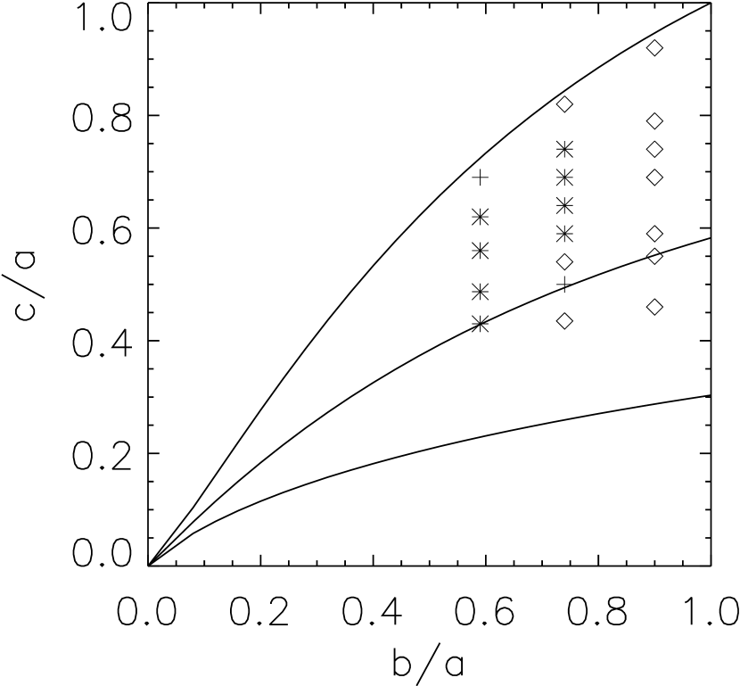
Figure 14: Results from our present investigation are summarized across the $(b/a,c/a)$ parameter domain from twenty separate dynamical simulations of compressible, adjoint configurations. The three solid curves are the same as in Figure 13. Asterisks denote violently unstable models, plus signs denote moderately unstable models, and diamonds denote stable models. The four models whose evolutions have been discussed in detail in the text can be identified by the $(b/a,c/a)$ parameters defining their initial shapes, as documented in Table 1: A010 (0.74,0.821); A067 (0.90,0.692); A134 (0.74,0.487); and A100 (0.59,0.487). Of the models identified here, only model A067 was constructed using the softer, $n=1$ polytropic EOS.

4 Conclusions and Discussions

We have conducted a survey of the nonlinear hydrodynamic stability of compressible triaxial configurations that are initially in quasi-equilibrium and share the same velocity field as that of Riemann S-type ellipsoids. Our simulations show that many of these models are indeed very good long-lived, quasi-equilibrium states. In addition, we have found that a turbulence-like dynamical instability arises over a fairly large region of the examined parameter domain (see Figure 14). This instability is probably the same instability observed in the late evolution of a neutron star that was driven to a bar-like structure by GRR forces (Ou, Tohline, & Lindblom, 2004). The characteristics exhibited by this instability and the domain it occupies in the examined parameter space agree qualitatively with the elliptical instability that has been discovered in previous linear studies of incompressible configurations (Lebovitz & Lifschitz, 1996). Therefore, we suspect that this instability is the elliptical instability that appears to develop generically in fluid flows with elliptical stream lines.

As a result of this instability, we found that all odd azimuthal modes grew on a dynamical time scale, but were dominated by the $m=1$ and $3$ modes, whose amplitudes eventually surpassed the $m=2$ bar-mode and destroyed the ellipsoidal structure of each violently unstable model. It appears that the growth rate for unstable modes is higher in models with smaller $b/a$ values. This makes sense because the elliptical instability ought to disappear in circular flows with $b/a=1$. In a linear analysis of the elliptical instability in Riemann S-type ellipsoids, Lebovitz & Lifschitz (1996) did not discuss the behavior of the $m=1$ mode. However, the appearance of an eccentric $m=1$ mode in accretion disks (Goodman, 1993; Ryu & Goodman, 1994) is consistent with our discovery here that the $m=1$ mode can also develop in compressible flows and drain energy from the $m=2$ mode.

The existence of the elliptical instability raises concerns regarding the final fate of neutron stars that encounter the GRR-induced secular bar-mode instability. According to previous theoretical investigations (Detweiler & Lindblom, 1977; Lai & Shapiro, 1995), such a star would be expected to evolve through a sequence of Riemann S-type ellipsoids toward the Dedekind sequence that has a vanishingly small pattern frequency as viewed from the inertial reference frame. However, Lebovitz & Lifschitz (1996) have shown that most of the Dedekind sequence falls in the parameter regime where fluid configurations should be susceptible to the elliptical instability; if any star enters this region of parameter space, the elliptical instability would set in on a dynamical time scale. It was unclear in the linear study of Lebovitz & Lifschitz (1996) whether the elliptical instability would be mild or violent in the nonlinear regime. This picture was partially answered by the nonlinear evolution of one rotating neutron star that was susceptible to the GRR-induced secular bar-mode instability (Ou, Tohline, & Lindblom, 2004); the bar-like configuration was observed to be destroyed very quickly when the pattern frequency of the bar dropped to nearly zero. The evolutions of compressible triaxial models presented in this paper further clarify what the nonlinear outcome will be of the elliptical instability. We have found that the instability can be violent and capable of destroying the ellipsoidal structure of the star. Therefore, it seems unlikely that a secularly unstable star driven by GRR forces will actually be able to evolve along a sequence of Riemann S-type ellipsoids toward a Dedekind-like configuration.

At the final stage of the evolution reported by Ou, Tohline, & Lindblom (2004), after the bar-like structure was destroyed and the star returned back to a nearly axisymmetric state with strong differential rotation, its $T/|W|$ value was still above the critical limit of $0.14$ for the secular bar-mode instability. Hence, it is possible that such a star would again attempt to evolve toward the Dedekind-sequence under the influence of GRR forces. Cycles of instability could continue until the star’s rotational energy is drained below the critical limit. If this picture is correct, it would provide a very interesting, recurrent source of gravitational-wave radiation for ground-based gravitational-wave detectors such as the Laser Interferometer Gravitational-wave Observatory (LIGO) and its sister instruments worldwide.

References

- Bayly (1986) Bayly, B. J., 1986, Phys. Rev. Lett., 57, 2160
- Cazes & Tohline (2000) Cazes, J. E., & Tohline, J. E. 2000, ApJ, 532, 1051
- Chandrasekhar (1969) Chandrasekhar, S. 1969, Ellipsoidal Figures of Equilibrium, New Haven, CT: Yale Univ. Press
- Chandrasekhar (1970) Chandrasekhar, S. 1970, ApJ, 161, 561
- Detweiler & Lindblom (1977) Detweiler, S., & Lindblom, L., 1977, ApJ, 213, 193
- Durisen & Tohline (1985) Durisen, R. H., & Tohline, J. E. 1985, in Protostars and Planets. II, ed. D. C. Black & M. S. Matthews (Tucson: Univ. of Arizona Press), 534
- Friedman & Schutz (1978) Friedman, J., & Schutz, B. F. 1978, ApJ, 222, 281
- Goodman (1993) Goodman, J. 1993, ApJ, 406, 596
- Lai & Shapiro (1995) Lai, D., & Shapiro, S. L. 1995, ApJ, 442, 259
- Lebovitz (1987) Lebovitz, N. R. 1987, Geophysical and Astrophysical Fluid Dynamics, 38, 15
- Lebovitz & Lifschitz (1996) Lebovitz, N. R., & Lifschitz, A. 1996, ApJ, 458, 699
- Lebovitz & Saldanha (1999) Lebovitz, N. R., & Saldanha, K. I. 1999, Physics of Fluids, 11, 3374
- Lubow, Pringle & Kerswell (1993) Lubow, S. H., Pringle, J. E., & Kerswell, R. R., 1993, ApJ, 419, 758
- Motl, Tohline, & Frank (2002) Motl, P. M., Tohline, J. E., & Frank, J. 2002, ApJS, 138, 121
- Ou (2006) Ou, S., 2006, ApJ, 639, 549 (Paper I)
- Ou, Tohline, & Lindblom (2004) Ou, S., Tohline, J. E., & Lindblom, L. 2004, ApJ, 617, 490
- Pierrehumber (1986) Pierrehumber, R. T., 1986, Phys. Rev. Lett., 57, 2157
- Ryu & Goodman (1994) Ryu, D., & Goodman, J., 1994, ApJ, 422, 269
- Shibata & Karino (2004) Shibata, M., & Karino, S., 2004, Phys. Rev. D, 70, 084022
- Tohline (2002) Tohline, J. E. 2002, ARA&A, 40, 349