Looking for Signs of Anisotropic Cosmological Expansion in the
High-z Supernova Data

Abstract

Several problematical epochs in cosmology, including the recent period of structure formation (and acceleration), require us to understand cosmic evolution during times when the basis of FRW expansion, the cosmological principle, does not completely hold true. We consider that the breakdown of isotropy and homogeneity at such times may be an important key towards understanding cosmic evolution. To study this, we examine fluctuations in the high-z supernova data to search for signs of large-scale anisotropy in the Hubble expansion. Using a cosmological-model-independent statistical analysis, we find mild evidence of real anisotropy in various circumstances. We consider the significance of these results, and the importance of further searches for violations of the cosmological principle.

I Introduction and Research Rationale

After a wave of successes in recent years, cosmology today is facing a series of potentially major turning points. The accepted standard model of the field, the concordance model refConcord , is a patchwork of detailed and observationally proven theories, interlaced with paradigms that are equally well accepted, though less well proven and far less detailed in terms of precise physical models. In the near future, new data will either bring these paradigms dramatically into focus, or will force great changes into the tightly interwoven concordance model.

Besides the unsolved problem of baryogenesis, the two most problematical epochs in cosmology both involve similar circumstances: they seek to understand the Friedmann-Robertson-Walker (FRW) expansion of the universe during phases in which the fundamental conceptual basis of FRW expansion, the Cosmological Principle (i.e., isotropy and homogeneity) refKT , does not completely hold true. The early such epoch (the pre-homogenization period) is usually handled with the Inflation paradigm refKT , and the late such epoch (post-CMB formation of large scale structure) is currently addressed with paradigms such as Vacuum Energy refKT , Quintessence refQuint (e.g., Tracker Quintessence refTrkQnt ), etc. Correct or not, these paradigms are not yet well constrained or proven in detail; and we take the position that it is no coincidence that the two least well understood epochs in cosmology happen to occur at times in which the Cosmological Principle loses its validity.

Demonstrating any direct theoretical link between the violation of isotropy and homogeneity, and solutions to specific cosmological problems, is beyond the scope of this current analysis; nor do we include here any investigation of the pre-homogenization period in the very early universe. What we focus upon here is the late epoch during which the CMB-era smoothness finally breaks down into clumpy structure. We seek to determine how seriously the Cosmological Principle is broken in the recent universe, and the tool we use for this purpose is the collection of high-redshift Type Ia supernova data used for measuring the cosmic acceleration (e.g., refRiess1 ), representing perhaps the best mapping of the expansion flow on very large scales. Measuring the extent of any irregularity in the smooth Hubble expansion would be a key step towards determining its significance (if any) in our understanding of cosmological concordance.

Theoretically, there remains room for new physics, since post-CMB evolution and the formation of large scale structure is by no means a “solved problem”. Despite the strengths of linear gravitational collapse models in a Cold Dark Matter/Dark Energy ($\Lambda_{\text{CDM}}$) universe refWMAP , there remain many loose ends, such as: the cuspy CDM halo problem, and the possible dearth of identifiable satellite-galaxy-sized structures in the local universe refPrim ; the overabundance of high-z clusters predicted by low-density $\Lambda_{\text{CDM}}$ models, implying actual values of $\Omega_{\text{M}}$ higher than those in the concordance model refXMM1 ; refXMM2 ; the unexpected existence of very massive galaxies at high-z refGenz ; the troubling, persistent tendency of Type Ia SNe data to indicate best-fit values of $\Omega_{\text{tot}}>1$ refBarris and/or (for Dark Energy) $w<-1$; the unknown behavior and composition of the Dark Energy itself (not to mention the Dark Matter) refTurner1 ; the possibility of non-Gaussian and hemisphere-asymmetric behavior in the WMAP data refNonGauss ; and the question of what is causing the lack of low-order multipole power in the CMB, as well as its rolling spectral index of fluctuations refWMAP .

Searching for meaningful anisotropy in the cosmic expansion is not without empirical justification. Well documented are the large discrepancies that have been historically found between different measurements of the Hubble Constant, yielding a broad and non-Gaussian distribution of results refCGR ; and though the error bars on $H_{0}$ have been greatly reduced over the years, even results quoted as demonstrating concordance (e.g., the agreement between values for $H_{0}$ found by WMAP and by the Hubble Key Project refWMAP ), remain tempered by the fact that different types of $H_{0}$ measurements (e.g., combining S-Z effect and cluster X-ray flux measurements) still give somewhat discordant values refWMAP . In addition, in the high-z supernova data used to prove cosmic acceleration, though the accelerating trend is statistically strong refRiess1 , there remain enormous fluctuations for the individual SNe scattered about that trend (to be shown below). While the bulk of such discrepancies are doubtless due to a number of factors unrelated to the expansion itself – e.g., systematic errors (theoretical and observational), poorly-understood physical processes causing variations in SN luminosity refSNvar , measurement difficulties leading to very large statistical errors, scarcity of data, etc. – it remains possible that at least some of this SN scatter (and some of the disagreement between different $H_{0}$ measurements) represents real physics, and appears due to unknown dependencies of the expansion rate on angular position in the sky, which has been virtually ignored up to now by cosmological research because of the assumption of isotropy.

Despite the broad assumption (and validity) of the Cosmological Principle in general, we are not the first to explore the possibility of meaningful cosmic anisotropy on the largest observable scales. Zehavi et al. refHubbBubb searched the early high-z supernova data (with marginal, positive results) for possible evidence that we might live in a local “bubble” of faster Hubble flow within a shell bounded by the local Great Walls. Alternatively, a detailed examination of the question by Lahav refOFRW led to some evidence of overall homogeneity, such as: agreement in shape and amplitude (except at the largest scales) between the 2dFGRS spectrum and a $\Lambda_{\text{CDM}}$ linear-regime perturbations model ref2dFOL ; the near-convergence between the CMB dipole and the IRAS galaxy clustering dipole refOFRW ; ref2MASSdipole ; some evidence (though conflicting) of an isotropic distribution of very distant radio sources; an upper limit (produced using substantial theoretical interpretation) on anisotopy of sources contributing to the X-ray background; the apparent absence of big voids in the Lyman-a forest (covering $1.8<z<4$, roughly); and, anisotropy constraints by Kolatt and Lahav refKOsne from Type Ia SNe. (Somewhat curious is this last result, in which Kolatt and Lahav interpret a mild rejection of isotropy at the $\sim 70\%-80\%$ confidence level as evidence for FRW behavior at these scales.) In short, there are a number of lines of evidence pointing towards isotropy and homogeneity on very large (sub-CMB) scales, though none of them are completely convincing at this time. The strongest reason for believing in extended FRW behavior long after the CMB epoch is still mainly a drive for concordance – a theoretical motivation, not empirical proof.

Direct probes of cosmic structure made by mapping the universe still remain inconclusive in demonstrating large-scale homogeneity. Despite perennial expectations of reaching scales large enough for which structure finally gives way to smoothness, evidence continues to be found for apparently real structure at ever-increasing scales. Examples include: the large “Local Hole”, a significant deficit of galaxies in the APM survey area, re-verified with 2MASS data, and implying possible non-Gaussian clustering on scales up to $\sim 300h^{-1}$ Mpc refFrith ; $\sim 200-300$ Mpc sized structure detected in the 2dF QSO redshift survey ref2dFQSO ; and the SDSS detection of the gigantic “Sloan Great Wall”, a structure 80% larger than the CfA Great Wall (450 Mpc wide) in comoving coordinates refUmap .

The implications of such results are debated: Mueller and Maulbetsch refSupSDSS claim that in contrast to other, earlier results, the supercluster and void structure in the SDSS data is well reproduced by high-resolution $\Lambda_{\text{CDM}}$ simulations; Miller et al. ref2dFQSO demonstrate (using a model requiring some bias of QSO distribution with respect to the Dark Matter distribution) that their 2dF QSO detection of very large structure does not provide any evidence of collapsed, non-linear structures on scales larger than 100 Mpc; and Gott et al. refUmap claim (counterintuitively, it may seem) that the detection of the unprecedentedly large Sloan Great Wall provides support for the expected approach to large-scale homogeneity (based upon an a posteriori argument that the size of Sloan Great Wall, despite being much larger than any previously known “single” structure, was not the largest possible structure that could have fit in the SDSS survey). Nevertheless, the overall lesson still remains: the transition from CMB-era smoothness to the recent, clumpy universe is still very poorly understood, and the potential importance of anisotropy and inhomogeneity in the “Dark-Energy-dominated” epoch of cosmic evolution continues to be an open question.

The immediate impetus for this analysis is the publication of a combined, standardized list of 230 Type Ia Supernovae refHzSN2 , containing extinction, redshift, luminosity distance and angular sky position data. Similarly to Kolatt and Lahav refKOsne , we search the SN data for statistical evidence of a lack of uniformity in the Hubble flow. What is different, however, is that we do not interpret our results according to any particular cosmological model. While they express their results in terms of variations in $H_{0}$, $\Omega_{\text{M}}$, etc., we instead ask a bare statistical question: “Have some regions of the universe been expanding faster than others?”, once the average Hubble evolution with respect to z is (empirically) removed. This has two advantages: it keeps our analysis much more independent of theoretical assumptions; and we avoid the problem of having to dilute data from a limited, noisy sample by dividing the statistical power of the results among 4 four different model parameters.

One other aspect of our analysis is that we separately consider SNe at “intermediate-z” ($.01<z<\sim.1-.2$), vs. “high-z” ($z>\sim.1-.2)$. We use different types of analyses because the former is distributed more evenly, giving better sky coverage; though the latter is of more interest here, since the higher-z SNe occupy more cosmologically-significant volumes of space, and correspond to look-back times closer to the onset of Hubble-flow acceleration.

Finally, we note that this conference proceedings paper is just a general overview of our results; we plan to present a more detailed discussion of our statistical methods and results in a future journal article.

II Preparation of Data for Analysis

The data analyzed here is taken from the work of Tonry et al. refHzSN2 , a compilation of Type Ia SN data from many sources, including the High-z Supernova Search Team (HZT), the Supernova Cosmology Project (SCP), and other researchers throughout the years. The total sample includes 230 SNe, presented in as uniform a fashion as possible, with a common calibration.

For most of our cosmological analysis, we apply the same data cuts as in refHzSN2 : we remove all SNe with $z<0.01$ (to minimize scatter from non-Hubble-flow peculiar motions), and we remove SNe known to be heavily extinguished (i.e., $\textit{A}_{V}<0.5$ mag, for SNe with listed $\textit{A}_{V}$ values). These cuts reduce the sample set from 230 to 172, but successfully eliminate many dramatic (and likely spurious) outliers from the cosmic expansion rate fits. Later, we will divide the data into groups of “mid-z” and “high-z” SNe; but for now we consider the entire sample.

The distance modulus (in Mpc) for each supernova is given as refWeinberg :

$$(m-M)=25+5~{}\text{log}(d_{L})=25+5~{}\text{log}(d_{L}H_{0})-5~{}\text{log}(H_{0})~{},$$ (1)

where $d_{L}$ is the supernova’s luminosity distance, and lists of log$(d_{L}H_{0})$ for all SNe are given in refHzSN2 .

The theoretical luminosity distance in an empty or coasting (i.e., $q_{0}=0$) universe would be refWeinberg :

$$D_{L}=\frac{cz}{H_{0}}(1+\frac{z}{2})~{},$$ (2)

with an expression similar to Eq. 1 for calculating the theoretical distance modulus, $(m-M)_{coasting}$. Any cosmic acceleration or deceleration is then found by computing the residuals, as follows (for the $i^{th}$ SN):

$$\Delta(m-M)_{i}\equiv\Delta_{i}=[(m-M)-(m-M)_{coasting}]_{i}=5~{}[\text{log}(d_{L}H_{0})-\text{log}(cz)-\text{log}(1+\frac{z}{2})]_{i}~{}.$$ (3)

In most analyses, these $\Delta_{i}$’s would then be used to find a best-fit cosmological model to be interpreted in terms of $\Omega_{m}$, $\Omega_{\Lambda}$, etc. But what we are interested in here is not finding best-fit model parameters, but in studying the scatter of the data around the average cosmological expansion (whatever that is, assuming it to be well defined), for potential signs of cosmic anisotropy and inhomogeneity. To do this in a purely statistical, model-independent way, we perform a very simple fit to the data, and then subtract this fit, $f(z)$, from the $\Delta_{i}$’s to compute the “modified residuals”:

$$\delta(m-M)_{i}\equiv\delta_{i}=[\Delta(m-M)-f(z)]_{i}~{}.$$ (4)

These $\delta_{i}$’s are reasonably independent of z, and can thus be used for SN statistical analysis.

A polynomial fit to the $\delta_{i}$ for the 172 SNe is shown in Figure 1, with a best-fit function of $f(z)=(0.586z-0.547z^{2})$. The essential physics is fairly well modeled (for this limited range of z) with just a 2${}^{\text{nd}}$-order polynomial, showing both the current cosmic acceleration and the earlier deceleration. This fit yields a $\chi^{2}$ of 230; a little bit high, but good enough for our purposes. The cosmological fits in refHzSN2 do somewhat better, but they achieve that partially by artificially enlarging the error bars (which are somewhat heuristically generated in the first place) to include a velocity uncertainty (or dispersion) of 500 km/sec. We do not do this here, since such a procedure actually obscures the effect which we are trying to study (i.e., their “noise” is our data).

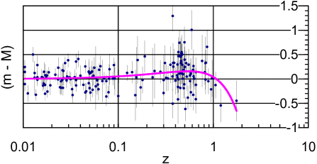
Figure 1: Residuals of $\Delta(m-M)$ for Supernovae, plot vs. best-fit $2^{nd}$-order polynomial, $y=0.586z-0.547z^{2}$.

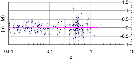
Figure 2: Modified residuals, $\delta(m-M)$, from Fig. 1 fit.

For any fit with a reasonable number of parameters, however, the SNe will always have tremendous scatter about the best-fit trendline. In this case, the index of fit refRossStat R is only 0.32, indicating that $\sim$70% of the variation in the data, roughly speaking, has nothing to do with this (or any similar) fit. Tonry et al. refHzSN2 note the extreme noisiness of this data, and deal with it by binning the SNe, and taking medians over each redshift bin. While this may be useful for the analysis of cosmological models, it once again is a procedure which masks the physics that we wish to study here.

A plot of our fit-removed $\delta_{i}$’s is shown in Fig. 2, depicting a similar-looking (though now visibly random) scatter. This is the main data that we analyze in this paper.

III Presentation of Results

Here we give a brief overview of some results of our Supernova analysis.

First, considering the “mid-z” (i.e., $.01<z<\sim.1-.2$) SNe data, we divide the SNe into 3 groups, depending upon their $\delta_{i}$ values: “high”, “mid”, or “low”. A plot of these data on the sky is shown in Fig. 3; and a modal analysis (using Spherical Harmonic modes) is depicted in Fig. 4, shown along with the modal decompositions of 300 randomly simulated skies, for comparison.

Some significant results here: the possible detection of a moderate dipole (larger than 80% of simulated skies); no evidence of a significant quadrupole mode (smaller than $\sim 70\%$ of simulated skies); and the possible detection of one or two especially large anisotropy modes, particularly the $Y_{33}$ mode (cosine phase). The structure of this specific mode is demonstrated in Fig. 5; and future analysis with more data will be crucial in determining whether this is a real sign of anisotropy in the cosmic expansion, or merely a random event from the decomposition of this data set into a large number of modes.

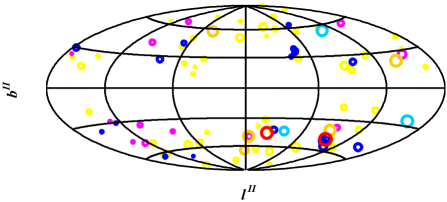
Figure 3: Hammer-Aitoff plot of $\delta(m-M)$ for SNe at $.01<z<.2$ (with bubble size $\propto z$), color-coded depending upon $\delta$ (blue for low values, yellow for medium values, red/pink for high values).

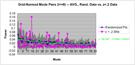
Figure 4: Spherical harmonic modal decomposition of $\delta(m-M)$ for $.01<z<.2$ SNe (pink), vs. modal decompositions for 300 simulated random skies (blue).

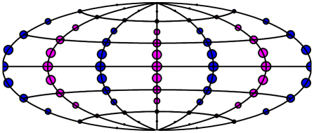
Figure 5: Single largest mode from the decomposition in Fig. 4, $Y_{33}Cosine$ (real mode, cosine phase).

In an attempt to interpret the dipole mode present in the data (if it is real), Figure 6 compares the direction of this dipole with a variety of other known, cosmologically-significant dipoles or significant directions – such as the CMB Dipole, and dipole hotspots/coldspots from 2Mass, IRAS, Local Group velocity, etc.; and the Milky Way center, the Great Wall, the Great Attractor, the Perseus-Pisces Supercluster, the Supergalactic Plane, etc. Simple inspection does not indicate any clear, obvious alignment of the dipole we have derived from the SN data with any of these other dipoles, though it is possible that the Supergalactic Plane does run through the hot/coldspots of this apparent SN dipole. In any case, future supernova data should more precisely determine the direction and magnitude of the SN dipole (if it exists), and determine whether or not there is any real correlation with other cosmic dipoles.

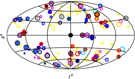
Figure 6: Comparison of dipole direction from the decomposition in Figs. 3 & 4, vs. various galactic, intergalactic, and cosmological dipoles.

Now we consider the “high-z” (i.e., $z>.1$) SNe data, again dividing it up into three groups, with “high”, “mid”, and “low” $\delta_{i}$ values. A plot of these data on the sky is shown in Fig. 7, with the sky roughly divided into 4 quadrants, for statistical comparison. (The kind of modal analysis done earlier for the intermediate-z SN data is not as appropriate here, due to the lack of any real “all-sky coverage” by the data.)

Statistical tests (t-tests refRossStat ) between the upper-left and lower-right quadrants (the quadrants with the most and highest-z SN data) show mild, positive evidence of an asymmetry between the quadrants, with an effective statistical significance of $\sim 1-1.8\sigma$ (depending upon the specific data cuts used).

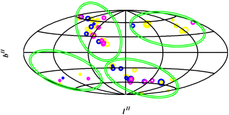
Figure 7: Hammer-Aitoff plot of $\delta(m-M)$ for SNe at $z>.1$ (with bubble size $\propto z$), color-coded depending upon $\delta$ (blue for low values, yellow for medium values, red/pink for high values). Data partitioned into 4 regions reflecting groupings in space and $z$.

Lastly, as is shown in Fig. 8, we re-partition the SNe data into smaller, more specific groupings (partitioning done somewhat arbitrarily, but with the partitions being made as similar as is feasible in sky area). In this case, statistical tests (ANOVA tests refRossStat ) again indicate mildly positive results ($\sim 1-2\sigma$, depending upon the specific data cuts) for real differences between the $\delta_{i}$ values – and thus the expansion rate histories – for SNe in different parts of the sky.

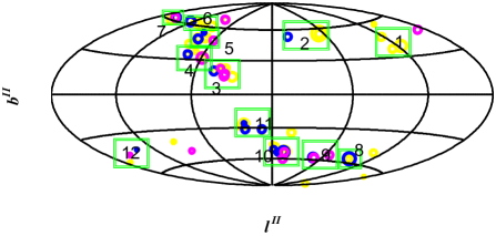
Figure 8: Same data as in Fig. 7, re-partitioned into more smaller, more numerous groupings.

IV Conclusions

We summarize these overall results as follows:

1. Given that Friedmann Robertson-Walker Cosmological Expansion depends upon the Cosmological Principle (Isotropy and Homogeneity), and that these assumptions break down in the recent universe (the Structure Forming and Accelerating Epoch), it is important to test the extent of this breakdown.

2. High-z Supernovae are likely the best probes for these tests, as long as angular information is considered and analyzed, not just sky-position-averaged behavior as a function of z.

3. For SNe at $.01<z<.2$, we find some evidence of a dipole (which the Supergalactic Plane may be passing through), as well as a largest (real Spherical Harmonic) Anisotropy mode of $Y_{33}$Cosine. But both findings are difficult to quantify in terms of statistical significance.

4. For SNe at $z>\sim.2$, we find some mild positive evidence for a “Dipole-like” Expansion Rate Anisotropy in opposite regions of the sky; and similar evidence for anistropies between smaller subdivided regions of the sky. But large gaps in sky coverage make these results hard to evaluate conclusively.

5. As more and better Supernova data are obtained (especially more all-sky coverage), we will be able to place more significant statistical limits on these potential anisotropies in the cosmological expansion.

- (1) M. Tegmark, M. Zaldarriaga, and A. J. S. Hamilton, Phys. Rev. D 63, 043007 (2001).
- (2) E. W. Kolb and M. S. Turner, The Early Universe (Addison-Wesley Pub. Co., Redwood City, CA, 1990).
- (3) L. Krauss, Quintessence (Basic Books, New York, NY, 2000).
- (4) P. Steinhardt, L. Wang, and I. Zlatev, Phys. Rev. Lett. 82, 896 (1999).
- (5) A. G. Riess et al., Astron. J. 116, 1009 (1998).
- (6) D. N. Spergel et al., Astrophys. J. Suppl. 148, 175 (2003).
- (7) J. R. Primack, astro-ph/0312549 (2003).
- (8) S. C. Vauclair et al., Astron. Astrophys. 412, L37 (2003).
- (9) A. Blanchard, M. Douspis, M. Rowan-Robinson, S. Sarkar, Astron. Astrophys. 412, 35 (2003).
- (10) R. Genzel et al., astro-ph/0403183 (2004).
- (11) B. J. Barris et al., Astrophys. J. 602, 571 (2004).
- (12) M. S. Turner, Int. J. Mod. Phys. A. 17, Suppl. Iss. No. 1, 180 (2002).
- (13) H. K. Eriksen, D. I. Novikov, P. B. Lilje, A. J. Banday, and K. M. Gorski, astro-ph/0401276 (2004).
- (14) G. Chen, J. R. Gott, and B. Ratra, Publ. Astron. Soc. Pac. 115, 1269 (2003).
- (15) F. X. Timmes, E. F. Brown, and J. W. Truran, Astrophys. J. 590, L83 (2003).
- (16) I. Zehavi, A. G. Riess, R. P. Kirshner, and A. Dekel, Astrophys. J. 503, 483 (1998).
- (17) O. Lahav, Class. Quant. Grav. 19, 3517 (2002).
- (18) O. Lahav and A. R. Liddle, astro-ph/0406681; Included in S. Eidelman et al., Phys. Lett. B 592, 1 (2004).
- (19) A. H. Maller, D. H. McIntosh, N. Katz, and M. D. Weinberg, Astrophys. J. 598, L1 (2003).
- (20) T. S. Kolatt and O. Lahav, Mon. Not. Roy. Astron. Soc. 323, 859 (2001).
- (21) W. J. Frith, P. J. Outram, and T. Shanks, astro-ph/0408011 (2004).
- (22) L. Miller et al., astro-ph/0403065 (2004).
- (23) J. R. Gott et al., astro-ph/0310571 (2003).
- (24) V. Mueller and C. Maulbetsch, astro-ph/0405288 (2004).
- (25) J. L. Tonry et al., Astrophys. J. 594, 1 (2003).
- (26) S. Weinberg, Gravitation and Cosmology (John Wiley & Sons, New York, NY, 1972).
- (27) S. M. Ross, Introduction to Probability and Statistics for Engineers and Scientists (John Wiley & Sons, New York, NY, 1987).