The Sunyaev-Zeldovich background

Abstract

The cosmic background due to the Sunyaev-Zeldovich (SZ) effect is expected to be the largest signal at mm and cm wavelengths at a resolution of a few arcminutes. We investigate some simple statistics of SZ maps and their scaling with the normalization of the matter power spectrum, $\sigma_{8}$, as well as the effects of the unknown physics of the intracluster medium on these statistics. We show that the SZ background provides a significant background for SZ cluster searches, with the onset of confusion occurring around $10^{14}h^{-1}M_{\odot}$ in a cosmology-dependent way, where confusion is defined as typical errors in recovered flux larger than 20%. The confusion limit, corresponds to the mass at which there are roughly ten clusters per square degree, with this number nearly independent of cosmology and cluster gas physics. Typical errors grow quickly as lower mass objects are included in the catalog.

We also point out that there is nothing in particular about the rms of the filtered map that makes it especially well-suited for capturing aspects of the SZ effect, and other indicators of the one-point SZ probability distribution function are at least as well suited for the task. For example, the full width at half maximum of the one point probability distribution has a field-to-field scatter that is about $60\%$ that of the $rms$.

The simplest statistics of SZ maps are largely unaffected by cluster physics such as preheating, although the impact of preheating is clear by eye in the maps. Studies aimed at learning about the physics of the intracluster medium will apparently require more specialized statistical indicators.

galaxies: clusters: general ; galaxies: intergalactic medium ; cosmology: cosmic microwave background

1 Introduction

The properties of the cosmic microwave background (CMB), and particularly its anisotropies, are a treasure trove of information about the fundamental cosmological parameters that define the large-scale structure of the Universe and about the early Universe physics that set the stage for the emergence of the present-day cosmic structures. As CMB experiments reach higher sensitivity (approaching $1\;\mu{\rm K}$) and higher resolution (approaching 1 arcminute) across a wide range of frequencies (from 20 to 900 GHz), they also hold forth the promise of providing new windows for probing the distribution of matter at redshifts $z\ll 1000$. This material is the dominant source of the temperature fluctuations in the CMB on scales less than 4 arcminutes.

The largest source of these small-scale anisotropies at the mm and cm wavelengths is expected to be the Sunyaev-Zeldovich (SZ) distortion from clusters of galaxies (Sunyaev & Zeldovich, 1972; Birkinshaw, 1999; Carlstrom et al., 2002). This distortion is caused by the inverse-Compton scattering of CMB photons by hot intracluster gas, and it has a characteristic spatial and spectral signature in CMB sky maps. The magnitude of the SZ effect from a galaxy cluster is determined by the integrated gas pressure along the line of sight; SZ anisotropies thus have the potential to yield valuable insights regarding the physical processes at play within clusters, especially those that have shaped the spatial and thermodynamic properties of the diffuse baryons.

The current measurements of the small-scale anisotropy by instruments such as the Cosmic Background Imager (CBI) (Mason, 2003) and the Berkeley-Illinois-Maryland Array (BIMA) (Dawson et al., 2002) are broadly consistent (Komatsu & Seljak, 2002; Holder, 2002a; Bond et al., 2005) with levels expected from the SZ effect, though the slight discrepancy in the normalization of the mass fluctuations $\sigma_{8}$ implied by these measurements versus those implied by other cosmological probes may be a harbinger of interesting times ahead (Doré et al., 2004). Current experiments such as the Sunyaev-Zeldovich Array (SZA) (Muchovej et al., 2006), the Atacama Cosmology Telescope (ACT) (Kosowsky, 2006), and the South Pole Telescope (SPT) (Ruhl & SPT collaboration, 2004) ought to be able to able to image the small-scale anisotropies with exquisite signal-to-noise.

Given their importance, considerable attention has been devoted to identifying approaches for quantifying, analyzing and interpreting these small-scale anisotropies in the CMB maps. Typically these have involved either constructing source counts as a function of source size or source flux density (e.g. Barbosa et al., 1996) or computing the SZ power spectrum (e.g. Cole & Kaiser, 1988). (We refer the reader to the review by Carlstrom et al., 2002 for a more detailed discussion of these two approaches as well as an extensive list of related references.) A hybrid approach was outlined in Diego & Majumdar (2004).

In this paper, we examine both these approaches. We show that the SZ background is effectively an irreducible contaminant that must be factored into the scan strategies for upcoming SZ survey experiments. We determine the mass scale below which SZ counts will be subject to confusion and show that the current generation of SZ experiments will be very close to being confusion limited if $\sigma_{8}=0.9$. We also investigate the “bandpower” approach to characterizing the SZ power spectrum. At first glance, this approach may appear to be a rather blunt measure, raising questions about its efficacy for providing useful information about the underlying sources of the anisotropies.

For these investigations, we generate synthetic maps of the SZ effect as we vary cluster gas physics and a single cosmological parameter, the normalization of the matter density power spectrum ($\sigma_{8}$). Our map-making algorithms and underlying assumptions are discussed in § 2. Our methodology is specifically tailored to capture the effects of projection and clustering of galaxy clusters but not substructure and asphericity within the clusters. Admittedly, the cluster profiles are not very realistic but since we are primarily concerned with the SZ background, we do not believe that this limitation is critical. On the contrary, since our maps are free of the ambiguities associated with determining whether one is looking at several objects in projection or a single object with multiple components, we are able to identify cleanly the influence of projection and clustering on the SZ maps. Furthermore, the regularity of cluster populations in X-ray properties (Nagai et al., 2007), which should be much more sensitive to substructure, suggests that substructure and asphericity are not likely to be large problems.

We use our SZ maps to investigate the SZ background as a source of contaminant for source counts extracted from a wide-field survey. Precisely determined SZ source counts are potentially sensitive tools for studying of the growth of structure over cosmic time, for determining the fundamental cosmological parameters, and for constraining unknown quantities such as the dark energy equation of state. The cosmological power of these surveys is crucially dependent (Majumdar & Mohr, 2003) on the relationship between the observable quantities (such as, flux and angular size) and the relevant intrinsic properties of the source population (such as mass). A significant strength of SZ source counts as a cosmological tool, the lack of redshift-dependent dimming, is also a weakness: the SZ sky will also consist of superposition of numerous weak distortions associated with largely unresolved clusters spanning a range of redshifts and mass scales. These background fluctuations can significantly distort the observable quantities associated with identified sources. In § 4, we comment on the resulting consequences for future SZ wide-field cluster surveys.

Next we look at current approaches to characterizing the SZ power spectrum. In reporting a power spectrum on a given scale, a complex map of numerous sources of varying amplitudes and scales is reduced to a single number, a “band-power”, characterizing the rms fluctuation amplitude in a SZ map filtered through some bandpass window centered about the scale of interest. For the primary CMB anisotropies, this type of characterization is well motivated, since the fluctuations are believed to Gaussian random and the statistical nature of a Gaussian random field is completely specified by its two-point correlation function or equivalently, its power spectrum. SZ fluctuations, however, are not Gaussian random and characterizing them via a power spectrum only makes sense in the limit of a large number of sources leading to the bulk of the anisotropy, where one might hope that the map becomes nearly Gaussian through the central limit theorem. Indeed, as we demonstrate in § 5, there is nothing about the rms or the variance of a filtered map that identifies it as especially well-suited for characterizing the SZ anisotropies. The variance has the nice property that it adds with the noise variance in a way that is independent of the shape of the probability distribution, but as the new generation of experiments begins to image the SZ background at high signal to noise this is not necessarily a large advantage. In fact, there are several alternate quantities derived from the one-point SZ fluctuation probability distribution function that allow for somewhat better cosmological discrimination, even in the simplest case where we restrict ourselves to reducing the richness of the SZ probability distribution (Zhang & Sheth, 2007) to a single number.

By restricting our study to one-point statistics of idealized cluster sources we have eliminated many real-world complications that are both important and confusing, such as substructure, detector noise, contamination by primary and secondary CMB anisotropies and foregrounds. However, this simplicity allows a clearer understanding of the impact of effects such as projection effects that would be difficult to clearly identify and isolate in full numerical simulations. Increasing the realism of the sky maps will be a necessary next step to be able to connect to real experiments in a meaningful way. However, we expect the results below to be robust.

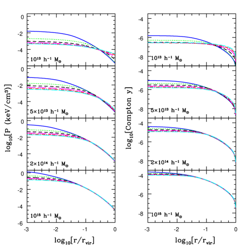
Figure 1: The left column shows, from top to bottom, the spherical pressure profiles for clusters of masses $1\times 10^{13}\;h^{-1}{\rm\;M}_{\odot}$, $5\times 10^{13}\;h^{-1}{\rm\;M}_{\odot}$, $2\times 10^{14}\;h^{-1}{\rm\;M}_{\odot}$, and $1\times 10^{15}\;h^{-1}{\rm\;M}_{\odot}$. In each panel, we show pressure profiles corresponding to $S_{\circ}=10$, $100$, $200$, $300$, $400$ and $500$ keV cm² (in descending order at $r/R_{v}=0.01$). The right column shows the corresponding projected Compton $y$ profiles. For a given cluster, increasing $S_{\circ}$ has two effects on the cluster’s Compton $y$ profile. The amplitude of the $y$ profile in the inner regions of the cluster diminishes while the signal in the outer regions increases. Both effects are the most pronounced for low cluster masses and high $S_{\circ}$. The lower mass clusters have corresponding shallower potential wells and the gas in these systems is more susceptible to rearrangement in response to feedback.

2 Mapmaking Methodology

We opt for an approach that uses semi-analytic methods to generate halo catalogs as a function of cosmological parameters, and use a well-studied analytic model for the distribution of diffuse gas in groups and clusters to populate the halos with baryons in a realistic fashion. Mechanically, this procedure is similar to that done by Kay et al. (2001), who used the Hubble Volume simulations to generate halo catalogs and will miss the effects of diffuse gas that are captured using hydrodynamical simulations (White et al., 2002; da Silva et al., 2000). Most of the anisotropy comes from bound objects (da Silva et al., 2001), although there are significant contributions to both the mean Compton $y$ and to the kinetic SZ effect expected from unbound gas .

We use the Pinocchio formalism (Monaco et al., 2002) to generate the halo catalogs. Starting with a realization of the initial linear density field within some specified volume, this algorithm not only predicts the mass function and the merger histories of the collapsed halos within the volume, but also provides information about their spatial locations. The results have been shown to be in excellent agreement with the results of full $N$-body simulations. Pinocchio, however, is computationally several orders of magnitude faster.

For the present study, we restrict our consideration to a reference cosmological model characterized by $\Omega_{m}=0.3$, $\Omega_{\Lambda}=0.7$ and $h=0.7$ but allow $\sigma_{8}$ to span the range from 0.6 to 1.0. For each value of $\sigma_{8}$, we generate six different simulation cubes of 256 $h^{-1}$ comoving Mpc on side, and output the corresponding halo catalogs at redshift intervals corresponding to 256 $h^{-1}$ Mpc in comoving distance. These simulation volumes are stacked to generate an integrated catalog of halos along a line-of-sight that correctly accounts for the significant evolution of cosmic structure as function of look-back time. Rather than simply stacking simulations corresponding to one realization, we randomly choose between one of the six volumes at each redshift, randomly select between one of three possible orientations and further apply a random periodic global translation to its content. Once the stack is assembled, we compile a list of all halos that fall within a $2^{\circ}\times 2^{\circ}$ field as seen by an observer at $z=0$. For each value of $\sigma_{8}$, we construct 100 realizations of the the $2^{\circ}\times 2^{\circ}$ sky field, and we only include halos with masses above $10^{13}h^{-1}M_{\odot}$ in the catalog. The mass threshold does not have a significant impact on the results. The SZ power spectrum is dominated by galaxy clusters of masses on the order of $10^{14}h^{-1}M_{\odot}$ (Holder, 2002b; Atrio-Barandela & Mücket, 1999). This field size is comparable in width to the “ACT Strip” (although much shorter in length), and of the same order as a typical SZA field.

Next, we populate each halo in the final catalog with hot diffuse baryons according to the analytic model of McCarthy et al. (2003). These models provide a simple, physically intuitive description of the intracluster medium subject to both heating due to accretion and infall, as well as non-gravitational heating events phenomenologically associated with, for example, starburst and AGN activity at the time when cluster galaxies are form, or AGN outbursts triggered by inflow of cooling gas once the cluster approaches a relaxed configuration.

In the standard hierarchical framework, the thermodynamic properties of the intracluster medium (ICM) are determined purely by heating due to accretion shocks and compression, and by radiative cooling. It has been known for a decade, however, that cluster models that include only these processes fail to reproduce both the observed stellar-to-gas mass ratio and the mean observed X-ray properties of the clusters (e.g. Lewis et al., 2000; Balogh et al., 2001; Babul et al., 2002; Voit et al., 2002; Lin et al., 2003; McCarthy et al., 2004). For instance, the observed X-ray luminosity-temperature ($L_{x}-T_{x}$) relation is steeper than predicted. Also, recent analytic and numerical investigations show that neither the cosmic halo-to-halo variations in the detailed structure of dark matter distribution of the cluster halos nor the effects of mergers can account for the relatively large scatter in the $L_{x}-T_{x}$ relation (Rowley et al., 2004; McCarthy et al., 2004; Balogh et al., 2006; Poole et al., 2007). On the other hand, models that, in addition to radiative cooling and accretion-related heating, also include early heating associated with AGN activity can account for most of the observed X-ray/SZE/optical scaling relations (c.f. Babul et al., 2002; Nath & Roychowdhury, 2002; McCarthy et al., 2002; McCarthy et al., 2003, 2004; Ostriker et al., 2005; Roychowdhury et al., 2005; Poole et al., 2007; McCarthy et al., 2007) but also for the real scatter in $L_{x}-T_{x}$ (McCarthy et al., 2004; Balogh et al., 2006). Additionally, this class of models can also resolve one of the most persistent problems in galaxy formation: the production of far too many high luminosity galaxies than observed (Benson et al., 2003). AGN feedback naturally produces an anti-hierarchical quenching of star formation in large galaxies, consistent with observations of galaxy down-sizing, due to the relatively late peak in ($z\approx 2$) in nuclear activity (Scannapieco et al., 2005).

Purely gravitational processes produces entropy profiles of the form $S(r)\propto r^{1.1}$ outside the cluster cores. This behaviour has been noted in numerical simulation studies of clusters (Lewis et al., 2000; Kay et al., 2004; Voit et al., 2005) and has also been observed in a wide range of clusters (Pratt & Arnaud, 2005; Piffaretti et al., 2005; Donahue et al., 2005; McCarthy et al., 2007). In the models of McCarthy et al. (2003), the extent of AGN heating is parameterized through the modification of the gas entropy profile, specifically through the introduction of an entropy core of amplitude $S_{\circ}$. The gas distribution in a halo is specified by the specific value of $S_{\circ}$ and requiring that the gas is in hydrostatic equilibrium. Under the assumption that $S_{\circ}$ varies from cluster to cluster, one can interpret the results as a providing a snapshot in time of the gas distribution in a halo. Unlike the more sophisiticated models of McCarthy et al. (2004, 2007), those described in McCarthy et al. (2003) do not track the evolution of $S(r)$ as a function of time. We have opted to used the more simpler models because by allowing for a variation in $S_{\circ}$, we are able to span the full range of plausible entropy profiles and gas distributions without having to concern ourselves with details of the heating mechanism and of the timing of the heating events in individual clusters.

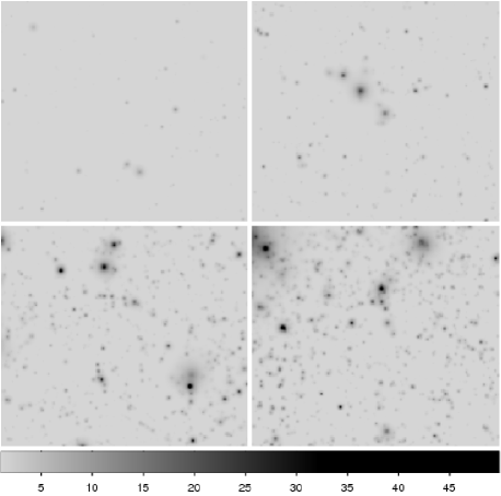
Figure 2: Examples of maps for different choices of $\sigma_{8}$. Each map is a randomly chosen realization and shows a square that is 0.85 degrees on a side. The values of $\sigma_{8}$ are 0.6 (top left), 0.7 (top right), 0.8 (bottom left), and 0.9 (bottom right) and the cluster model is chosen to have $S_{\circ}=200$ keV cm². The map resolution is 14” and the shown region is only the central part of a map that is 2 degrees on a side. The units of the map are $10^{6}\times y$, not temperature units. To convert to Rayleigh-Jeans temperature in units of $\mu K$, multiply by 5.46.

The nomalization, slope (shape) and the scatter in the various SZ effect and X-ray scaling relations as well as the variations in the shape of X-ray surface brightness profiles of massive clusters suggest that $S_{\circ}$ spans the range from $\sim 0-10$ keV cm² to $\sim 400-500$ keV cm², with the entropy profiles for the $S_{\circ}=10$ keV cm² models being in excellent agreement with the observed entropy profiles of the classical cool core clusters (Donahue et al., 2005; McCarthy et al., 2007). We account for this range by generating a series of spherical pressure profiles corresponding to different values of $S_{\circ}$ for each of the halos in our final catalogs and use these these to obtain circularly symmetric Compon $y$ profiles characterized by cluster mass, redshift and entropy parameter $S_{\circ}$. All of the physics of the SZ effect is contained in the Compton $y$ profiles:

$$y(\mathbf{\theta})={\sigma_{T}\over m_{e}c^{2}}\int P_{e}(\mathbf{r})dl,$$ (1)

where $\mathbf{\theta}$ is the projected position from the cluster center, $\sigma_{T}$ is the Thompson scattering cross section, $P_{e}(\mathbf{r})\equiv n_{e}(\mathbf{r})kT_{e}(\mathbf{r})$ is the electron pressure of the ICM at the three dimensional position $\mathbf{r}$ from the cluster center, and the integral is performed over the line of sight ($l$) through the cluster. For example, the change in the temperature of the CMB due to the SZ effect is (Carlstrom et al., 2002)

$$\Delta T(\mathbf{\theta})=T_{CMB}y(\mathbf{\theta})\left[x{e^{x}+1\over e^{x}-1}-4\right],$$ (2)

where $x=h\nu/kT_{CMB}\approx\nu/56.85$ GHz, and $T_{CMB}=2.728$ (Fixsen et al., 1996). In the long wavelength regime (the Rayleigh-Jeans limit), $\Delta T(\mathbf{\theta})\approx-2T_{CMB}y(\mathbf{\theta})$

In Fig. 1, we show both the spherical pressure profiles and the corresponding projected Compon $y$ profiles for clusters of different masses and a range of $S_{\circ}$. Typically, as $S_{\circ}$ is increased, the reorganization of the gas within the halo leads to the reduction in the ampltitude and the flattening of Compon $y$ profiles in the cluster centers. This reorganization also results in an increase in the amplitude of the Compon $y$ profiles outside the cluster cores, but the fractional change is small and the effect is negligible for clusters with $M\lower 2.15277pt\hbox{$\;\buildrel>\over{\sim}\;$}10^{14}\;{\rm\;M}_{\odot}$. For smaller mass systems, however, the rearrangement of the gas leads to a sizeable increase in Compon $y$ profiles over the bulk of the cluster.

To construct our sky maps, we start with a given catalog of halo corresponding to a specific value of $\sigma_{8}$. We use the positions of the halos in the catalogs to locate the cluster centers in a $2^{\circ}\times 2^{\circ}$ sky field. Next, we choose a value for $S_{\circ}$, select the associated 2D Compton $y$ profile for each of the halos in the catalog, and place these at corresponding positions in the sky field to generate an SZ map. We do this for all catalogs, ending up with 100 realizations of the SZ sky maps for each ($\sigma_{8}$, $S_{\circ}$) pair. As already noted, we explore $\sigma_{8}$ values ranging from $0.6$ to $1.0$, and for each of $\sigma_{8}$, consider several different values of $S_{\circ}$. We adopt the $\sigma_{8}=0.9$, $S_{\circ}=200$ keV cm² model as our reference case. Not all the values of $\sigma_{8}$ in the range being considered are in concordance with either the constraints from the cluster abundance studies (Henry, 2004) or the recent microwave background results (Spergel et al., 2003; Spergel, 2006); nevertheless it is still instructive to consider the full range in order to probe the dependence on $\sigma_{8}$.

Fig. 2 shows four SZ sky maps generated using a model where $S_{\circ}=200$ keV cm² and four different values of $\sigma_{8}$. The power of SZ statistics as a probe of $\sigma_{8}$ is apparent by eye from this figure, as the amount of structure is a strong function of $\sigma_{8}$. These maps were selected as the first realization of each ensemble and the central region was selected for display.

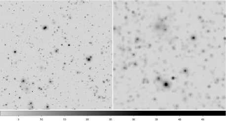
Figure 3: Examples of maps for extreme choices of entropy floor: 10 keV cm² (left) and 500 keV cm² (right). Each map is a randomly chosen realization and shows a square that is 0.85 degrees on a side. Both maps assume $\sigma_{8}=0.9$. The map resolution is 14” and the shown region is only the central part of a map that is 2 degrees on a side. The units of the map are $10^{6}\times y$, not temperature units. To convert to Rayleigh-Jeans temperature in units of $\mu K$, multiply by 5.46.

There are two noteworthy items regarding our SZ maps that we would like to draw attention to. First, our sky maps are constructed assuming that all the clusters have the same value of $S_{\circ}$. In principle, we ought to have allowed for a cluster-to-cluster variation in $S_{\circ}$ as suggested by the scatter in the SZ effect and X-ray observations; however, the shape of the distribution in $S_{\circ}$, much less its dependence on cluster mass and redshift, is not known. To this end, we have adopted the simplest possible distribution for $S_{\circ}$ and investigate the possible implications for variations in $S_{\circ}$ by constructing maps with different values of $S_{\circ}$. Second, although we have peculiar velocity information for each of the halos, we do not make use of these in the present study. Therefore, our maps only incorporate the thermal SZ effects, not the kinetic SZ effects. The latter are expected to approximately an order of magnitude smaller and their inclusion would only have a marginal effect on the issues of interest to us in the present study.

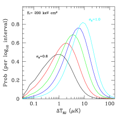
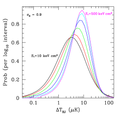
Figure 4: Distribution of pixel values for unfiltered maps (14” resolution) as a function of $\sigma_{8}$ (left) and amount of preheating (right). There are some empty pixels (not shown) due to the neglect of unbound gas, with the fraction of empty pixels increasing with lower $\sigma_{8}$. In the left panel, from left to right the curves show increasing $\sigma_{8}$ from 0.6 to 1.0 in steps of 0.1; the right panel shows increasing levels of preheating at a fixed value of $\sigma_{8}=0.9$, from left to right showing $S_{\circ}=10,100,200,300,400,500$ keV cm².

The distribution of pixel values in the unfiltered maps captures some of the details apparent in the maps. As $\sigma_{8}$ increases the number of sources increases, as does the number of bright sources (see Figs. 4 and 3). Increasing the value of $S_{\circ}$ has the effect of making clusters less centrally concentrated, leading to fewer very bright pixels but more pixels at intermediate values, as the outer regions of the clusters are somewhat enhance (as indicated by the crossover around 70 $\mu K$). The utility of SZ surveys as a cosmological probe is apparent in that the number of bright pixels is clearly very sensitive to $\sigma_{8}$ but not very sensitive to non-gravitational gas physics. But it is also clear that high resolution $\mu K$ imaging of the SZ effect will provide insight into the detailed physical processes at play in clusters.

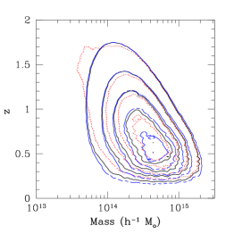
Figure 5: The SZ power spectrum (left) and the differential contribution to SZ power spectrum, $dc_{\ell}/d\ln{M}dz$, at $\ell\sim 4500$ (right), for our models with $\sigma_{8}=0.9$ and varying levels of preheating. At high $\ell$ the models from top to bottom have entropy floors of 10,100,200,300,400,500 keV cm² in the left panel; the right panel shows entropy floors of $S_{\circ}=10$ (blue, dashed curve), 200 (black, solid) and 400 keV cm² (red, dotted curve). See text for details on cluster models. The contours in the right panel are linearly spaced.

3 The SZ Angular Power Spectrum

The distribution of the CMB temperature fluctuations due to the SZ effect on the celestial sphere is conventionally written as an expansion in terms of the spherical harmonic functions,

$${\Delta T\over T_{CMB}}(\theta,\phi)=\sum_{\ell,m}a_{\ell m}Y_{\ell m}(\theta,\phi)$$ (3)

and quantified by the coefficients $a_{\ell m}$, or by the angular power spectrum of the SZ effect: $C_{\ell}=\langle|a_{\ell m}|^{2}\rangle$. For small angles ($\ell\ga 50$) the flat sky approximation should be sufficient, where the multipole expansion can be replaced by a Fourier expansion (White et al., 1999) with $e^{2\pi i\vec{u}\cdot\vec{x}}$ such that $2\pi|u|=\ell$.

To gain some intuition for the SZ background, we can use a Press-Schechter (Press & Schechter, 1974) approach to estimate the form of the SZ power spectrum. Ignoring correlations between clusters, the power spectrum can be thought of as a superposition of random sources. Each source has a profile in Fourier space that is modulated by a phase factor due to its random position on the sky. At a given position in Fourier space, the superposition of many sources with random phases leads to a random walk in the real and imaginary components. The power spectrum is thus given by

$$C_{\ell}=\int dz{dV\over dz}\int dM{dn\over dM}|\Delta\tilde{T}(\ell,M,z)|^{2}$$ (4)

where $\Delta\tilde{T}$ is the Fourier transform of the SZ profile, $dV/dz$ is the comoving volume per unit redshift and $dn/dM$ is the comoving number density of objects of mass $M$. We use the number density indicated by fits to numerical simulations (Jenkins et al., 2001). We obtain the Fourier transform of the SZ profile using the $y$ profiles of the preheated models and a Hankel transform routine to take advantage of the circular symmetry of the model clusters.

In left panel of Fig. 5, we plot angular SZ power spectra as rms contribution per unit interval $[\ell(\ell+1)C_{\ell}/2\pi]^{1/2}$ for our reference model ($\sigma_{8}=0.9$, $S_{\circ}=200$ keV cm²) as well as the full range of preheated models with the same $\sigma_{8}=0.9$, with the $S_{\circ}$ parameter ranging from $10$ to 500 keV cm². In the right panel, we show the differential contribution to the SZ power spectrum, $dc_{\ell}/d\ln{M}dz$, at $\ell\sim 4500$ for the same three models. The effects of feedback at moderate levels results in the well-known damping of the SZ power on all scales but most pronouncedly, on small scales (Holder & Carlstrom, 2001; Lin et al., 2004). As illustrated in the right panel of Fig. 5, the power on intermediate scales primarily comes from clusters of a few times $10^{14}h^{-1}M_{\odot}$ at moderate redshift and as a result these scales are little affected by preheating. We note, however, that our calculations do not include the impact of unknown amount of depletion of electrons due to star formation as a function of redshift and/or mass. With only $\la$15% of the baryons in stars (Lin et al., 2003) in the local universe, we do not expect this effect to alter our results.

The level of preheating has very little effect on intermediate scales; the SZ effect is most sensitive to gas dynamics on scales of several hundred kpc, while non-gravitational physics is most effective on scales of tens of kpc or less. While non-gravitational physics can be quite effective at changing the small-scale power in the SZ effect, it is extremely difficult to affect the overall energy budget of the cluster in a significant way.

4 Confusion Noise for SZ Surveys

We start by using our simulated SZ maps to investigate the SZ background as a source of contaminant for source counts extracted from a wide-field survey. A glance at the maps makes it clear that the maps are highly non-Gaussian. At the same time, the extended nature of the sources is also apparent, indicating that the maps are also not a simple collection of points. Consequently, the very strength of the SZ effect that makes it particular attractive probe of cosmology and structure formation, the lack of redshift-dependent dimming, also means that the SZ sky will contain, in addition to well-defined source signals, a background comprised of the superposition of numerous weak distortions associated with largely unresolved clusters spanning a range of redshifts and mass scales. These background fluctuations act as a significant contaminant for the source counts (Schulz & White, 2003), potentially distorting the observable quantities associated with identified sources and limiting the power of the SZ source counts as a probe of cosmology and growth of structure since the efficacy of the measure depends on there being a well-defined relationship between the observable quantities (such as, flux and angular size) and the intrinsic properties (such as, mass) of the source population.

As a first step towards analyzing our simulated maps, we apply a finite band-pass filter, equivalent to an annulus in $\ell$ space, to the sky maps such that only Fourier modes (in the flat sky approximation) with $3000<\ell<6000$ are retained. This corresponds to an ideal CMB experiment reporting a single band power over the specified range in $\ell$. In principle, this approach can be generalized to mock up the results for specific CMB experiment by applying the corresponding window function to the ensemble of maps. We choose a single idealized band for the purpose of providing a concrete demonstration.

The filtering scheme that we have adopted is a crude but a reasonably accurate representation of the typical matched filter for upcoming SZ surveys (Holder, 2004). The matched filter is designed to suppress both the large-scale signal due to the primary CMB fluctuations and the very small-scale signal largely dominated by detector noise. With sufficiently sensitive multifrequency surveys, the primary CMB signal could be removed spectrally and the large scales need not be filtered out, but the simplest approach would be to take advantage of the separation of spatial scales and use this information to remove the CMB through spatial filtering.

In order to characterize the nature of the SZ background, we investigate the total SZ flux in the filtered sky maps at the projected position of each input halo as a function of the halo mass. In Fig. 6 we show the fractional errors in the reconstructed flux, defined as

$${\Delta S_{\nu}\over S_{\nu,true}}={S_{\nu,map}-S_{\nu,true}\over S_{\nu,true}},$$ (5)

where $S_{\nu,true}$ is the SZ flux expected in the filtered map if the halo under consideration was the only source present, and $S_{\nu,map}$ is the measured flux in the filtered map. The fractional error is very small at the projected positions of massive clusters, but the same is not true at the other end of the mass scale. At the projected positions of the low mass systems, the SZ flux has significant contribution from nearby neighbours, particularly neighbours with large footprints in the sky. This, in turn, leads to a very large scatter in the fractional error. At the risk of being repetitive, we stress that these maps do not include pixel noise or primary CMB fluctuation and the only noise here comes from sources overlapping with each other.

At this point, the approach of this paper is a huge advantage compared to numerical simulations. As a function of mass and redshift we can calculate the exact SZ signal expected in the filtered maps by simply filtering the models used to generate the maps. There is no additional noise due to substructure, triaxiality, mergers, or large scale filamentary gas. This is a pure test of projection effects.

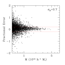
Figure 6: Fractional error in the SZ flux [calculated as (map-model)/model] in the $2^{\circ}x2^{\circ}$ filtered sky maps at the projected position of the input halos in all 100 realizations of the $S_{\circ}=200$, $\sigma_{8}=0.9$ model (right) and $\sigma_{8}=0.7$ (left). The dotted lines show $\pm 20\%$ errors. Each panel shows 10000 clusters selected randomly from the ensemble of maps.

We define a mass scale at a given redshift as resolved if the $rms$ fractional error is less than 20%. The limiting mass scale below which confusion becomes important is slightly above $10^{14}h^{-1}M_{\odot}$ for the $S_{\circ}=200$, $\sigma_{8}=0.9$ model. As shown in Fig. 7, this “confusion mass scale” varies with the redshift, typically decreasing as a function of redshift, and also scales with $\sigma_{8}$. We define the confusion mass averaged over redshift as the constant mass threshold at which the $rms$ fractional error of SZ flux estimates above that mass is 20%, roughly corresponding to being comparable to the noise level for a $5\sigma$ detection. The confusion mass calculated this way can be well approximated by

$$M_{conf}=10^{14}h^{-1}M_{\odot}(\sigma_{8}/0.75)^{2.5}\ .$$ (6)

This confusion mass scale is not very sensitive to the details of the cluster thermodynamics. This is because the dominant source of confusion is due to clusters with nearly similar masses, and as long as the limiting mass is not close to the mass scale where feedback induces a qualitative change in the nature of the gas distribution in the halos, feedback will impact halos with massess at, just above, and just below the “confusion scale” similarly, leaving the mass scale itself relatively unchanged.

To understand the origin of this background better, we took the simulation volumes for our fiducial model and randomized the halo positions within each box. We then repeated the mapmaking exercise using the randomized halo positions to construct the sky maps. The confusion levels did not, however, change appreciably in these randomized sky maps, confirming that the effect described here is a true background, and not simply one caused primarily by the correlated distribution of structure in the vicinity of the objects of interest.

Finally, we note that the background described above is effectively an irreducible background, caused by structure on the same scale and (obviously) the same spectral behaviour as the desired objects. For this reason, we anticipate that this background is going to be the dominant source of noise for future generations of SZ survey instruments. As a rule of thumb, the confusion limit corresponds to roughly ten objects per square degree; in this regime catalog construction will be straightfoward and the results robust. This surface density is not too dissimilar from that of typical confusion estimates in astronomy (Hogg, 2001), which is usually quoted as of the order 25 beams per source. In this case, the beam is set by characterisic scale of clusters rather than the observing beam, and is therefore only approximate. However, 25 beams per source and a density of 10 clusters per square degree implies a typical “beam” extent (diameter) of 4’ per cluster. At a cosmological distance this corresponds to a radial extent of roughly $0.5h^{-1}$ Mpc. The characteristic scale of the clusters contributing to the confusion is therefore roughly half the virial radius.

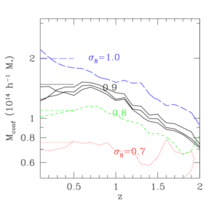
Figure 7: Mass scale below which confusion becomes a significant contaminant (see text for details) as a function of source redshift. From top to bottom, the curves correspond to $\sigma_{8}=$ 1.0 ( dot-dashed), 0.9 (solid), 0.8 (dashed), and 0.7 (dotted). The horizontal lines at the left edge of the plot identifies the constant limiting mass that corresponds to 10 clusters per square degree in each model. For $\sigma_{8}$=0.9 there are three lines shown, corresponding to $K_{\circ}=10,200,500$ keV cm².

If we define the confusion mass instead as the mass which leads to ten objects per square degree for our cosmology, the confusion mass becomes $M_{conf}=10^{14}h^{-1}M_{\odot}\times(\sigma_{8}/0.77)^{2.7}$, remarkably close to the scaling obtained from the maps. This suggests that this really can be treated as a confusion limit and that the effective beam size set by the galaxy cluster themselves is on the order of 4 arcminutes.

For a catalog defined by a fixed threshold relative to the detector noise, the scaling of $M_{conf}$ with $\sigma_{8}$ given above leads to bit of a paradox. At high values of $\sigma_{8}$, there are many more clusters per square degree and therefore, the Poisson noise is much lower. At the same time, confusion sets in at a higher mass threshold, making the task of constructing a catalog more challenging by increasing the rate of false positive detections. At low values of $\sigma_{8}$, the threshold scale for confusion is lower, allowing for the construction of very clean catalogs; however, because of the dearth of massive systems in low $\sigma_{8}$ cosmologies the resulting catalogs will be much more susceptible to Poisson noise.

The current generation of SZ survey experiments are expected to have noise levels that allow imaging of clusters that are very close to the confusion limit, on the order of $2\times 10^{14}h^{-1}M_{\odot}$. If $\sigma_{8}$ is near 1.0, then there is not much to be gained by improving the sensitivity, as these experiments will then be simply imaging the SZ background at higher signal to noise. On the other hand, if $\sigma_{8}$ is near 0.7, then the confusion mass is lower by nearly a factor of 3; assuming that the SZ flux scales as $M^{5/3}$ (the self-similar scaling) this translates into the confusion limit being at a flux threshold that is nearly 5 times lower. Real experiments have other concerns, such as radio and IR point sources, atmosphere subtraction, detector noise, ability to do other CMB science, etc., but the cosmological scaling of the SZ background could be an important consideration for survey designs.

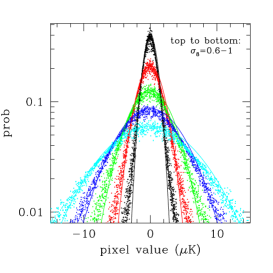
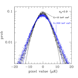
Figure 8: Probability distribution functions of pixel values in filtered ($3000<\ell<6000$) maps for models with $S_{\circ}=200$ keV cm² and $\sigma_{8}$=0.6,0.7,0.8,0.9,1.0 (top to bottom) [Left] and for $\sigma_{8}=0.9$ and $S_{\circ}$ =10,500 keV cm² [Right]. Results for all 100 realizations of each model are shown. Solid lines show Gaussians with the same FWHM as the mean of the 100 realizations for each model.

5 Comparison of Map Statistics

Experiments often report the power in a band, which we take to be $3000<\ell<6000$ in our case. This corresponds to the variance of a map that has been filtered in Fourier space such that only modes within an annulus in $\ell$ space have been retained. The variance provides the complete description of the signal in the filtered map if the distribution of the pixel values is Gaussian. In Fig. 8, we plot the histogram of the values of pixels in our sky map for the each of the 100 realizations of models with $S_{\circ}=200$ keV cm² and $\sigma_{8}$ spans the range from 0.6 to 1.0 (top to bottom). We will discuss this plot further in the next section. Here, it suffices to note that the the distribution of pixel values is, in general, not a Gaussian. The filtered map, therefore, contains much more information than represented by the variance, and of course, there is much more information on the sky than in a single filtered map. However, we shall restrict ourselves to analyzing sky maps filtered as described above and will further restrict the discussion to one-point statistics.

Variance is an example of such a measure and as noted, it completely captures all the information in sky maps where the pixel distribution is Gaussian. However, in the case of non-Gaussian distributions, the variance has its limitations. For example, the variance is very sensitive to the tails of the distribution, much more so than, for example, the full-width at half-maximum (FWHM) of the distribution. The two measures are somewhat complementary. Ideally, one would like to have a simple one-point statistical measure that is, for example, less sensitive to gas physics and more discrimating between cosmological models as well as an indicator that is able to isolate the effects of gas physics regardless of the cosmology, etc. Here, we investigate the mean absolute value, FWHM, variance, skewness and kurtosis. We normalize all these statistics such that they are equivalent for Gaussian statistics:

$\sigma_{var}=\sqrt{\langle x^{2}\rangle}$	$\hat{s}=\langle x^{3}\rangle/\sigma_{var}^{3}$
$\sigma_{fwhm}\equiv{\rm FWHM}/2.35$	$\hat{k}=\langle x^{4}\rangle/\sigma_{var}^{4}$
$\sigma_{abs}\equiv 1.25\,\langle|x|\rangle$

The quantities in the left column correspond to skewness and kurtosis, respectively. Also, we remind the reader that the filtered map has zero mean by construction, so there is no sensitivity to the mean Comptonization.

The SZ power spectrum is known to be a sensitive function of $\sigma_{8}$ (Komatsu & Seljak, 2002; Komatsu & Kitayama, 1999), so we first study the scalings of the various one-point statistical measures with $\sigma_{8}$.

As a first step, we plot in Fig. 8 the histogram of the values of pixels in our sky map for the each of the 100 realizations of models with $S_{\circ}=200$ keV cm² and $\sigma_{8}$ spanning the range from 0.6 to 1.0 in steps of 0.1 (top to bottom). Overall, the distribution of pixel values in the sky maps becomes progressively broader and more non-Gaussian as $\sigma_{8}$ is increased,

In the filtered maps, the effects of the entropy floor are small, as shown in the right panel of Fig. 8. The distributions are very similar, indicating that the power spectrum in Fig. 5 is giving a fair representation of the effects of preheating.

There is a significant degree of scatter from realization to realization, as can be seen in Fig. 8, due to the Poisson noise in the number of massive clusters. The strongly non-Gaussian wings are also largely due to these massive clusters, rendering $\sigma_{var}$ an increasingly poor statistic. We illustrate this in Fig. 8 by plotting, for each $\sigma_{8}$, a Gaussian with the same FWHM as the mean of the 100 realizations (solid curve). In addition to $\sigma_{var}$, we also consider two other one-point measures: $\sigma_{fwhm}$ and $\sigma_{abs}$. The behaviour of the variance and all the other measures are summarized in Table 1. All indicators scale roughly as $\sigma_{i}\propto\sigma_{8}^{n_{i}}$ with $n_{i}=7$, as suggested by (Komatsu & Kitayama, 1999). Note that results are presented with a proportionality symbol as a reminder that depletion of electrons through star formation will lead to a reduction of the SZ effect.

Interestingly, increasing the amplitude of the entropy floor drives the distribution towards slightly less non-Gaussianity. This arises in part because the central Comptonization is reduced in each cluster, reducing the number of high-$y$ points. However, the effect is very small. The scaling of the skewness with entropy floor is only $\propto S_{\circ}^{-0.2}$ and the kurtosis only scales as $\propto S_{\circ}^{-0.3}$.

In interpreting Table 1 it is useful to consider the field-to-field variance of the statistical indicator, shown in the final column for the particular case of $\sigma_{8}=0.9$, as well as in Fig. 9 . As a statistical indicator, the ideal probe would be a strong function of the parameter of interest with small scatter. All the indicators of $\sigma$ have roughly the same scaling with $\sigma_{8}$, so the scatter is the best comparison tool. For an input $\sigma_{8}$ of 1, the scatter in $\sigma_{var}$ indicates that a typical map will give a 25% estimate of this parameter, leading to a constraint on $\sigma_{8}$ from a single 2x2 degree field that is on the order of 7%. Using a better estimator with 15% scatter, such as the full-width half-maximum, would lead to an estimate on the order of 4%. Of course, these estimates ignore pixel noise and primary CMB contamination and are highly idealized. However, using only a single “bandpower” the cosmological power of the SZ background is promising.

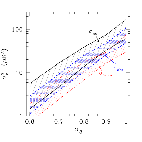
Figure 9: Distribution of variances in filtered maps ($3000<\ell<6000$) of size 2 degrees on a side as a function of $\sigma_{8}$ assuming fiducial gas evolution ($S_{\circ}=200$ keV cm². The 95% intervals are shown for three different map statistics: $\sigma_{var}^{2}$ (black solid), $\sigma_{fwhm}^{2}$ (red dotted), and $\sigma_{abs}^{2}$ (blue dashed).

Table 1: Summary of statistical indicators of filtered ($3000<\ell<6000$) SZ maps

statistic	$\sigma_{8}$		$\sigma_{x}/x$
	scaling (mean)		2x2 sq deg
$\sigma_{var}^{2}(\mu K^{2})$	$\propto$	$101\sigma_{8}^{7.1}$	0.	23
$\sigma_{abs}^{2}(\mu K^{2})$	$\propto$	$74\sigma_{8}^{7.2}$	0.	16
$\sigma_{fwhm}^{2}(\mu K^{2})$	$\propto$	$47\sigma_{8}^{7.3}$	0.	15
skewness	$1.5\sigma_{8}^{-0.4}$		0.	3
kurtosis	$22\sigma_{8}^{-0.8}$		0.	5

6 Summary and Future Work

SZ studies face a fundamental confusion limit coming from the superposition of many faint sources that becomes significant at a sky surface density of roughly ten clusters per square degree. By using spherical analytic halos of known properties we have isolated and quantified the confusion due purely to line of sight superpositions of SZ sources.

The existence of the SZ confusion limit is a challenging limitation to the ability to study low-mass systems with the SZ effect. Projection effects will require that any study of systems much below $10^{14}h^{-1}M_{\odot}$ will be necessarily statistical in nature, through such things as cross-correlations with optical, X-ray, or lensing maps, or stacking of many clusters to increase the signal to noise.

The SZ confusion limit found here should not be strongly impacted by the current uncertainty in cluster gas physics, since it is fundamentally determined mainly by the source density. If all clusters were simply scaled, the relative flux between sources just above and just below the confusion limit will not be changed. Even allowing a mass-dependent depression or enhancement in flux will only be important if it is more dramatic than the exponential suppression in the mass function at high masses.

We have shown that the variance is a crude tool to apply to SZ maps, and that better cosmological discrimination is possible with the fwhm or the mean absolute value and that in general the one point PDF of SZ maps is likely to be a rich dataset. There is almost certainly a much better single number that best captures the SZ pdf as a function of parameters, but the future will probably be better served by using a more complete treatment of the SZ joint pdf.

The work here only looked at a single parameter, $\sigma_{8}$, and it would be instructive to extend this work to include a host of other parameters, such as $\Omega_{m}$ and dark energy properties, to see how different parameters affect the SZ pdf. This is ongoing work. However, even looking at only one parameter it is clear that the SZ background for cluster surveys is a function of cosmology and calibrating a selection function using only a limited set of cosmological models is dangerous.

The amount of substructure in clusters could be sensitive to $\sigma_{8}$ and using “realistic” cluster profiles from N-body simulations that include hydrodynamics and astrophysics will be required to understand the details of the SZ background. At the same time, it must always be kept in mind that the SZ background is being largely produced by objects that are currently barely studied observationally; the properties of these objects have not been used to tune numerical simulations.

Ultimately, the distribution of SZ values and their spatial correlations will connect to source counts as a function of redshift, which suggests that the SZ “power spectrum,” whether using the variance or some better statistic, can benefit significantly from crude redshift estimates of all pixels, and not just the brightest few pixels. This is under investigation; a complete investigation of the multiwavelength characteristics of every position on the sky is a large undertaking.

The SZ background will soon be imaged at high resolution. We have demonstrated that there is a wealth of cosmological and astrophysical information in this signal, perhaps most obviously evident from a glance at the maps shown in Figs. 2 and 3. This wealth of information will allow for great advances in our cosmological and astrophysical understandings, but it is clear that the large recent advances in instrumentation must now be matched by advanced new tools for interpreting the signals.

This work was supported by the Natural Sciences and Engineering Research Council (Canada) through the Discovery Grant Awards to GPH and AB. GPH would also like to acknowledge support from the Canadian Institute for Advanced Research and the the Canada Research Chairs Program. IGM acknowledges support form a NSERC Postdoctoral Fellowship. AB acknowledges support from the Leverhulme Trust (UK) in the form of the Leverhulme Visiting Professorship. Both AB and GPH would like to thank CITA and IAS for the hospitality shown to them during their visit during the course of this study.

References

- Atrio-Barandela & Mücket (1999) Atrio-Barandela F., Mücket J. P., 1999, ApJ, 515, 465
- Babul et al. (2002) Babul A., Balogh M. L., Lewis G. F., Poole G. B., 2002, MNRAS, 330, 329
- Balogh et al. (2006) Balogh M. L., Babul A., Voit G. M., McCarthy I. G., Jones L. R., Lewis G. F., Ebeling H., 2006, MNRAS, 366, 624
- Balogh et al. (2001) Balogh M. L., Pearce F. R., Bower R. G., Kay S. T., 2001, MNRAS, 326, 1228
- Barbosa et al. (1996) Barbosa D., Bartlett J. G., Blanchard A., Oukbir J., 1996, A&A, 314, 13
- Benson et al. (2003) Benson A. J., Bower R. G., Frenk C. S., Lacey C. G., Baugh C. M., Cole S., 2003, ApJ, 599, 38
- Birkinshaw (1999) Birkinshaw M., 1999, Phys. Rep., 310, 97
- Bond et al. (2005) Bond J. R., Contaldi C. R., Pen U.-L., Pogosyan D., Prunet S., Ruetalo M. I., Wadsley J. W., Zhang P., Mason B. S., Myers S. T., Pearson T. J., Readhead A. C. S., Sievers J. L., Udomprasert P. S., 2005, ApJ, 626, 12
- Carlstrom et al. (2002) Carlstrom J. E., Holder G. P., Reese E. D., 2002, ARA&A, 40, 643
- Cole & Kaiser (1988) Cole S., Kaiser N., 1988, MNRAS, 233, 637
- da Silva et al. (2000) da Silva A. C., Barbosa D., Liddle A. R., Thomas P. A., 2000, MNRAS, 317, 37
- da Silva et al. (2001) da Silva A. C., Kay S. T., Liddle A. R., Thomas P. A., Pearce F. R., Barbosa D., 2001, ApJ, 561, L15
- Dawson et al. (2002) Dawson K. S., Holzapfel W. L., Carlstrom J. E., Joy M., LaRoque S. J., Miller A. D., Nagai D., 2002, ApJ, 581, 86
- Diego & Majumdar (2004) Diego J. M., Majumdar S., 2004, MNRAS, 352, 993
- Donahue et al. (2005) Donahue M., Horner D. J., Cavagnolo K. W., Voit G. M., 2005, Entropy Profiles in the Cores of Cooling Flow Clusters of Galaxies, astro-ph/0511401
- Doré et al. (2004) Doré O., Hennawi J. F., Spergel D. N., 2004, ApJ, 606, 46
- Fixsen et al. (1996) Fixsen D. J., Cheng E. S., Gales J. M., Mather J. C., Shafer R. A., Wright E. L., 1996, ApJ, 473, 576
- Henry (2004) Henry J. P., 2004, ApJ, 609, 603
- Hogg (2001) Hogg D. W., 2001, AJ, 121, 1207
- Holder (2002a) Holder G. P., 2002a, ApJ, 578, L1
- Holder (2002b) Holder G. P., 2002b, ApJ, 580, 36
- Holder (2004) Holder G. P., 2004, ApJ, 602, 18
- Holder & Carlstrom (2001) Holder G. P., Carlstrom J. E., 2001, ApJ, 558, 515
- Jenkins et al. (2001) Jenkins A., Frenk C. S., White S. D. M., Colberg J. M., Cole S., Evrard A. E., Couchman H. M. P., Yoshida N., 2001, MNRAS, 321, 372
- Kay et al. (2001) Kay S. T., Liddle A. R., Thomas P. A., 2001, MNRAS, 325, 835
- Kay et al. (2004) Kay S. T., Thomas P. A., Jenkins A., Pearce F. R., 2004, MNRAS, 355, 1091
- Komatsu & Kitayama (1999) Komatsu E., Kitayama T., 1999, ApJ, 526, L1
- Komatsu & Seljak (2002) Komatsu E., Seljak U., 2002, MNRAS, 336, 1256
- Kosowsky (2006) Kosowsky A., 2006, New Astronomy Review, 50, 969
- Lewis et al. (2000) Lewis G. F., Babul A., Katz N., Quinn T., Hernquist L., Weinberg D. H., 2000, ApJ, 536, 623
- Lin et al. (2004) Lin K.-Y., Woo T.-P., Tseng Y.-H., Lin L., Chiueh T., 2004, ApJ, 608, L1
- Lin et al. (2003) Lin Y.-T., Mohr J. J., Stanford S. A., 2003, ApJ, 591, 749
- Majumdar & Mohr (2003) Majumdar S., Mohr J. J., 2003, ApJ, 585, 603
- Mason (2003) Mason B. S. e. a., 2003, ApJ, 591, 540
- McCarthy et al. (2002) McCarthy I. G., Babul A., Balogh M. L., 2002, ApJ, 573, 515
- McCarthy et al. (2007) McCarthy I. G., Babul A., Bower R. G., Balogh M. L., 2007, MNRAS, submitted
- McCarthy et al. (2003) McCarthy I. G., Babul A., Holder G. P., Balogh M. L., 2003, ApJ, 591, 515
- McCarthy et al. (2004) McCarthy I. G., Balogh M. L., Babul A., Poole G. B., Horner D. J., 2004, ApJ, 613, 811
- McCarthy et al. (2003) McCarthy I. G., Holder G. P., Babul A., Balogh M. L., 2003, ApJ, 591, 526
- Monaco et al. (2002) Monaco P., Theuns T., Taffoni G., 2002, MNRAS, 331, 587
- Muchovej et al. (2006) Muchovej S., Carlstrom J. E., Cartwright J., Greer C., Hawkins D., Hennessy R., Joy M., Lamb J. W., Leitch E. M., Loh M., Miller A. D., Mroczkowski T., Pryke C., Reddall B., Runyan M., Sharp M., Wood D., 2006, ArXiv Astrophysics e-prints
- Nagai et al. (2007) Nagai D., Vikhlinin A., Kravtsov A. V., 2007, ApJ, 655, 98
- Nath & Roychowdhury (2002) Nath B. B., Roychowdhury S., 2002, MNRAS, 333, 145
- Ostriker et al. (2005) Ostriker J. P., Bode P., Babul A., 2005, ApJ, 634, 964
- Piffaretti et al. (2005) Piffaretti R., Jetzer P., Kaastra J. S., Tamura T., 2005, A&A, 433, 101
- Poole et al. (2007) Poole G. B., Babul A., McCarthy I. G., Fardal M. A., Bildfell C. J., Quinn T., Mahdavi A., 2007, MNRAS, submitted
- Pratt & Arnaud (2005) Pratt G. W., Arnaud M., 2005, A&A, 429, 791
- Press & Schechter (1974) Press W., Schechter P., 1974, ApJ, 187, 425
- Rowley et al. (2004) Rowley D. R., Thomas P. A., Kay S. T., 2004, MNRAS, 352, 508
- Roychowdhury et al. (2005) Roychowdhury S., Ruszkowski M., Nath B. B., 2005, ApJ, 634, 90
- Ruhl & SPT collaboration (2004) Ruhl J., SPT collaboration 2004, in Zmuidzinas J., Holland W. S., Withington S., eds, Millimeter and Submillimeter Detectors for Astronomy II The south pole telescope. SPIE, pp 11–29
- Scannapieco et al. (2005) Scannapieco E., Silk J., Bouwens R., 2005, ApJ, 635, L13
- Schulz & White (2003) Schulz A. E., White M., 2003, ApJ, 586, 723
- Spergel et al. (2003) Spergel D. N., Verde L., Peiris H. V., Komatsu E., Nolta M. R., Bennett C. L., Halpern M., Hinshaw G., Jarosik N., Kogut A., Limon M., Meyer S. S., Page L., Tucker G. S., Weiland J. L., Wollack E., Wright E. L., 2003, ApJS, 148, 175
- Spergel (2006) Spergel D. N. et. al., 2006, asto-ph/0603449
- Sunyaev & Zeldovich (1972) Sunyaev R. A., Zeldovich Y. B., 1972, Comments on Astrophysics and Space Physics, 4, 173
- Voit et al. (2002) Voit G. M., Bryan G. L., Balogh M. L., Bower R. G., 2002, ApJ, 576, 601
- Voit et al. (2005) Voit G. M., Kay S. T., Bryan G. L., 2005, MNRAS, 364, 909
- White et al. (1999) White M., Carlstrom J. E., Dragovan M., Holzapfel W. L., 1999, ApJ, 514, 12
- White et al. (2002) White M., Hernquist L., Springel V., 2002, ApJ, 579, 16
- Zhang & Sheth (2007) Zhang P., Sheth R. K., 2007, MNRAS, submitted