The evolution of submillimetre galaxies: two populations and a redshift cut-off

Abstract

We explore the epoch dependence of number density and star-formation rate for submillimetre galaxies (SMGs) found at $850\,\mu$m. The study uses a sample of 38 SMG in the GOODS-N field, for which cross-waveband identifications have been obtained for 35/38 members together with redshift measurements or estimates. A maximum-likelihood analysis is employed, along with the ‘single-source-survey’ technique. We find a diminution in both space density and star formation rate at $z>3$, closely mimicking the redshift cut-offs found for QSOs selected in different wavebands. The diminution in redshift is particularly marked, at a significance level too small to measure. The data further suggest, at a significance level of about 0.001, that two separately-evolving populations may be present, with distinct luminosity functions. These results parallel the different evolutionary behaviours of LIRGs and ULIRGs, and represent another manifestation of ‘cosmic down-sizing’, suggesting that differential evolution extends to the most extreme star-forming galaxies.

1 Introduction

‘Submillimetre galaxies’ (SMGs) represent a major population of massive star-forming galaxies at high redshift (e.g. Hughes et al. 1998; Blain et al. 2002). Found in limited-area sky surveys at $850\,\mu$m with the Submm Common-User Bolometric Array (SCUBA; Holland et al. 1999) on the James Clerk Maxwell Telescope, they are believed to be dust-enshrouded starbursts, with the dust heated by UV radiation from young stars. They may be the distant early equivalents of the local prodigious star-formers, the ULIRGs and LIRGs (‘Ultra-Luminous IR Galaxies’, ‘Luminous IR Galaxies’, Sanders & Mirabel 1996). SMGs appear to carry much of the star-formation rate density (SFRD) of the early Universe on their shoulders. Understanding these objects is thus fundamental to our understanding of galaxy formation. Several attempts have been made to track their contribution to the global SFRD as a function of epoch (e.g. Lilly et al., 1999; Chapman et al., 2005). These efforts have been hampered by incomplete cross-waveband identifications and hence the subsamples which have redshifts have been biased. Recently, Pope et al. (2005, 2006) succeeded in identifying 35 out of a sample of 38 SMGs from the SCUBA survey in the GOODS(Great Observatories Origins Deep Survey)-N field, and secured redshift estimates for all identifications. It is the object of this paper to use this sample to form a picture of the space density of these SMGs, and of the epoch dependence of both their space density and the corresponding SFRD.

The distinctive feature of the spectral energy distributions of SMGs is the dominance of the cold-dust spectrum, approximately that of a $\beta\simeq 1.5$ greybody at $35\,$K, peaking (rest frame $\nu I_{\nu}$) at frequencies near $3200\,$GHz, wavelengths near $90\,\mu$m. Such a spectrum implies that the K-correction is generally negative (i.e. we ascend the Rayleigh-Jeans tail as the object moves to higher redshifts), and that there is nothing to stop such objects being visible out to redshifts of 5 or more (e.g. Blain & Longair, 1993). However, the redshift distribution of SMGs appears to peak around $\sim$ 2.2, with little high-redshift tail beyond 4 (Chapman et al., 2005; Pope et al., 2006), so that there is qualitative evidence for a redshift diminution at early epochs. One of the aims of this paper is to quantify this diminution.

The wide-spread phenomenon of ‘cosmic down-sizing’ appears to be at variance with the idea of hierarchical build-up of galaxies. The emerging picture is that although dark matter haloes build up hierarchically, the behaviour of the baryons within these haloes is much more complicated. In cosmic down-sizing, the dominant activity becomes carried by more numerous, lower-luminosity, lower-mass objects at progressively later times. The ‘down-sizing’ (Cowie et al., 1996) originally described how dominant star formation in galaxies shifted from luminous rare galaxies at earlier epochs to more numerous and less luminous galaxies at recent epochs. In addition to star formation, cosmic down-sizing is now known to apply to other phenomena: AGN activity in X-ray QSOs (Ueda et al., 2003) and in radio galaxies (where it has been known for 40 years in the guise of ‘differential evolution’; Longair 1966), and SFR in ULIRGs+LIRGs (Pérez-González et al., 2005; Le Floc’h et al., 2005; Chary, 2006). This paper examines whether the concept further extends to SMGs and the ‘cold dust’ star formation rate (SFR) associated with them.

2 The submillimetre sample

2.1 The GOODS-N supermap

Currently, the largest SMG sample which is almost completely identified is from the GOODS-N field: all SCUBA data from several extensive imaging campaigns in the GOODS-N field have been combined into one 850-$\mu$m map, referred to as the ‘supermap’ (see Borys et al. 2003 and references therein). This supermap has noise properties that vary strongly with position, but this can be accounted for in the source extraction procedure.

The most recent published version of the supermap contains 35 $850\,\mu$m sources detected above $3.5\sigma$ and satisfying a flux ‘de-boosting’ threshold (Pope et al., 2006). Subsequent to this work, the inclusion of additional two-bolometer chopping photometry data in the supermap has resulted in three new $850\,\mu$m sources, two of which have secure identifications. The sample therefore totals 38; description of changes to the supermap as a result of these new data together with identification of the three sources is in Pope (2007). Appendix A gives the relevant data for these three sources.

It is important in the present context to be clear as to why the GOODS-N supermap yields a complete and unbiased sample. The issue is covered in previous papers (Pope et al. 2006 and references therein), and we reiterate and summarize the points here.

The supermap is in fact a maximum-likelihood estimate of the flux of a point source centered on each pixel. We take all the available data, from whatever observing mode, to obtain this estimate. To do this we use the beam-shape, as well as the chop information, as discussed in previous papers (Borys et al., 2003; Pope et al., 2005). The beauty of this approach is that we can include jiggle-maps with different chops as well as the scan-map, and we can also fold in photometry data in exactly the same way. Several checks were carried out to show that the different estimates for specific sources agree with each other, and that the statistics of the data going into each pixel are well behaved. There is no evidence of any bias from this procedure, except for the usual flux boosting, which occurs when a signal-to-noise threshold is applied to low S/N source data drawn from a steep source count. To account for this, we followed the Bayesian approach of Coppin et al. (2005), which reduces to a correction to the signal and noise of a source, dependent separately on that signal and noise. This method also has been extensively tested. The procedure allows an estimate of the fraction of sources which may not be real (subject to some interpretation of what constitutes a ‘source’ when approaching the confusion limit), and the expectation is that there are only 1 or 2 such objects. The de-boosting procedure led to removal of a handful of objects, most of which are in fact likely to be real, but for each of them the chances of being simply a noise excursion is not small. These are precisely the sorts of ‘$3-3.5\sigma$’ sources with relatively high noise which plagued earlier SMG follow-up work. After such sources are removed the final catalogue is very reliable [as we have confirmed with AzTEC (Astronomical Thermal Emission Camera; Perera et al., in preparation) and MAMBO (Max Planck Millimetre Bolometer; Greve et al., in preparation) maps of the GOODS-N field].

The resulting 38 sources, we believe constitute the most carefully compiled and complete sample of submm objects currently available.

With regard to comparing the sources in our list with the results obtained for radio-detected SMGs in GOODS-N by Chapman et al. (2005), our view is that these are complementary studies. The Chapman et al. sample relies heavily on pointed photometry towards optically-faint radio sources only. The resulting data have been extremely useful for understanding the properties of some SMGs, but unfortunately the sample is hard to use in a statistical sense, because there is no way to assess how biased it is, how complete it is, or what fraction of the sources might be interlopers.

As an example of how all data were included in the supermap, some of our sources, including two of the of the new ones, are from pointed photometry data. However, what we have done is to include all of these data in the new super-map, treating these data in precisely the same way as all the others, using the same source extraction threshold and de-boosting procedure. The main point is that this process includes all of the bolometers, and not just the central one, so that what we are effectively doing is adding under-sampled images to parts of the super-map. Given that there are 37 bolometers, the fact that the central one happened to be pointed at a specified place is not particularly relevant. These additional photometry data simply help the S/N in the supermap in an inhomogeneous way, which is easily tracked through estimation of the accompanying noise map. That we do not recover some of the Chapman et al. (2005) sources is just because they fail our source extraction criteria – for an individual pointed observation, it may be reasonable to take $3\sigma$ or less as a detection threshold, but such low values cannot be used when examining an entire map.

2.2 Identifications: the final sample

Using the multi-wavelength data available in GOODS-N, likely counterparts were found for $35/38$ of the SMGs. Full details on the identification process can be found in Pope et al. (2006). In brief: we searched for counterparts to the SMGs within a search radius of 8 arcseconds using primarily the radio, Spitzer MIPS (Multi-band Imaging Photometer) and IRAC (Infrared Array Camera) data. A counterpart is considered secure if it has a probability of random association, $P$, less than 5 per cent. The probabilities of random association are given in Table A2 of Pope et al. (2006) with the exception of the two new identifications. These two new identifications (Table 2), GN39 and GN40, have random-association probabilities of 0.02 and 0.003, respectively, and therefore qualify as secure. In fact 23/35 sources have secure ($P<0.05$) counterparts and we thus expect that at most one of these will be an incorrect identification. The rest of the counterparts, 12/35, are less secure, with $0.05<P<0.2$. However, when we combine the probabilities of these less secure identifications, we expect only 1.3 incorrect identifications amongst them. For our total sample of 35 SMGs identifications, we therefore expect at most 2–3 incorrect counterparts. As we describe in §3 and 5, we have folded this uncertainty into our analysis.

The extensive optical and infrared data yielded reliable photometric redshifts in the absence of spectroscopic redshifts (Pope et al., 2006); 17 SMGs in the sample have spectroscopic redshifts and the remaining 18 have optical or Spitzer photometric redshift estimates. Optical photometric redshifts of these SMGs were shown to be accurate by Pope et al. (2005). Pope et al. (2006) used the Spitzer photometry to derive model-independent estimates of the redshifts for sources without reliable optical photometric redshifts (9/35 sources). These redshifts were found to be accurate to $\sigma(\Delta z/(1+z))=0.07$.

This sample of 35 objects is the basis for the following analysis of space density. Throughout, we use a concordance cosmology with $\Omega_{\rm tot}=1.0$, $\Omega_{\rm m}=0.3$, $\Omega_{\Lambda}=0.7$ and $h=0.7$.

3 Exploring space distribution

For each SMG, we calculated the specific submm luminosity (at rest frame, $850\,\mu$m) using only the $850\,\mu$m flux and the redshift, and assuming a greybody spectral energy distribution with emissivity $\beta=1.5$ and dust temperature $T=35\,$K. While there will be some scatter in $T$ and $\beta$, these values provide a good description of the data as found in a number of submm surveys (Chapman et al., 2005; Kovács et al., 2006; Pope et al., 2006).

The objects are shown in a luminosity–redshift ($L\,{-}\,z$) plot in Fig. 1. It is clear from this figure that some standard luminosity function analyses will not work. The unique geometry means that the $1/V_{\rm max}$ method in particular is problematic, because most sources ‘see’ no survey limit. Moreover, beyond establishing the reality of evolution or otherwise, the $1/V_{\rm max}$ method is poorly suited to small samples. We therefore adopt a maximum-likelihood approach, as first advocated by Marshall et al. (1983) and used recently in the detailed analysis of X-ray QSOs by Ueda et al. (2003).

Figure 1: The $L\,{-}\,z$ plane for all 35 SMGs. The curved lines represent the 35 different survey cut-offs for these objects; every one of the objects lies above its cut-off line and these cut-off lines differ because of the differences in local noise properties in the supermap. Dividing the sample at the median value in log($L$) (see §5), black lines /dots represent the lower-luminosity objects; blue lines/dots represent the higher-luminosities, and dot size is representative of log($L$). Note the remarkable form of these cut-off lines; some of these objects can be seen out to effectively infinite redshifts because of the inverse K-correction. This plot already suggests the basic result – a dearth of luminous sources below $z\simeq 1.5$ and a dearth of weaker sources above $z\simeq 3$. The plot shows also how the ‘single-source-survey’ technique works. Taking the solid dot as a representative source, the heavy curve represents its individual survey cut-off, and in this instance the calculation of space density is for a redshift range 1.5 to 2.5. The function $\Omega_{i}(l,z)$ is shown as the green area, over which it has a constant value equal to the individual area relevant to the single source (see text); the function is zero (red) elsewhere.

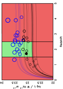
Thus, following Marshall et al. (1983), consider the sample as a single homogeneous set of $i$ objects, for which $\rho(z,L)(\partial V/\partial z)dzdL$ is the number in volume element $(\partial V/\partial z)dz$ in luminosity element $dL$. The sky fraction $\Omega_{i}(z,L)$ accessible to each object $i$ is unique – each of our objects is: (a) observable over an area of different physical size; and (b) has its own flux-density limit line in the $L\,{-}\,z$ diagram. This factor $\Omega_{i}(z,L)$ is thus essential in introducing the feature of the single-source-survey (Wall et al., 2005) by which each object is treated as having unique access to the $L\,{-}\,z$ plane (Fig. 1). The treatment is analogous to the final survey having been done as 35 individual surveys finding a single source each. The unique area accessible to each object on the $L\,{-}\,z$ plane is multiplied by its unique effective survey area to determine the final value of its $\Omega_{i}(z,L)$. This effective survey area is a function solely of flux density, with the relation as determined by Blake et al. (2006).

The $\cal L$(ikelihood) function for the $i^{\rm th}$ object is the probability of observing one object in its $(dz,dl)$ element times the probability of observing zero objects in all other $(dz,dl)$ elements accessible to it. The Poisson model is the obvious one for the likelihood:

$$f(x:\mu)=\frac{{\rm e}^{-\mu}\mu^{x}}{x!},$$ (1)

where $\mu$ is the expected number. If $x=1$, the function is $\mu{\rm e}^{-\mu}$ and if $x=0$ it is ${\rm e}^{-\mu}$.

With $\rho(z,L)$ as the full description of space density,

$$\mu=\lambda(z,L)\,dz\,dL,\ \ \mbox{for}\ \ \lambda=\rho(z,L)\Omega(z,L)(\partial V/\partial z).$$ (2)

Hence

$${\cal L}=\prod_{i}^{N}\lambda(z_{i},L_{i})\,dzdL\,e^{-\lambda(z_{i},L_{i})\,dz\,dL}\prod_{j\neq i}^{N}e^{-\lambda(z_{j},L_{j})\,dz\,dL}\!,$$ (3)

where $i$ denotes the elements of the $(z,L)$ plane in which SMGs are present and $j$ denotes all others. From this, if $S=-2\,\ln\cal{L}$, then

$$S = -2\sum_{i=1}^{N}\,\ln\rho(z_{i},L_{i})$$ (4)

$$+\sum_{i=1}^{N}\int_{z}\int_{L}\rho(z,L)\Omega_{i}(z,L)\frac{\partial V}{\partial z}\,dz\,dL+\mbox{constant.}$$

Consider simple factorizable density evolution of the form $\rho(L,z)=\rho(z{=}0,L)\cdot\phi(z)$. In this formulation we adopt a power-law luminosity function,

$$\frac{dN}{dL}=\rho(L,z)=\frac{\rho_{0}}{L_{*}}\,\phi(z)\,\left(\frac{L}{L_{*}}\right)^{-\alpha}\!.$$ (5)

With $l\equiv L/L_{*}\,$, we have the local luminosity function as $\rho(z{=}0,L)=(\rho_{0}/L_{*})\,l^{-\alpha}$. For the evolution function we again adopt a power-law, $\phi(z)=(1+z)^{k}$.

If we substitute these assumptions into equation (4) and set the derivative with respect to $\rho_{0}$ to zero, we get a maximum-likelihood estimate for $\rho_{0}$:

$$\rho_{0}=\frac{N}{\sum_{i=0}^{N}\int_{z}\int_{l}(1+z)^{k}\,l^{-\alpha}\,\Omega_{i}(z,l)\,(\partial V/\partial z)\,dz\,L_{*}dl}.$$ (6)

Putting this back into equation (4) gives

$$S = -2\sum_{i}^{N}\ln[(1+z_{i})^{k}\,l_{i}^{-\alpha}]$$ (7)

$$+2N\,\ln\sum_{i}^{N}\int_{z}\int_{l}(1+z)^{k}\,l^{-\alpha}\,\Omega_{i}(z,l)\,\left(\frac{\partial V}{\partial z}\right)\,dz\,dl$$

$$+(2N-2N\,\ln N).$$

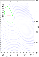
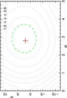
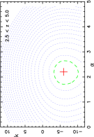
Inspection of Fig. 1 shows immediately that a single-power-law function to describe density evolution will not work. The density of points clearly rises with increasing redshift before $z=2$ and falls after $z=3$. Accordingly, we calculated the value of this likelihood function using a grid in ($k,\alpha$) for broad slices in redshift, with results shown in Fig. 2. This figure shows that: (a) the slope of the luminosity function does not change drastically with redshift; and (b) $k$, the $(1+z)$ exponent, changes from values around 5 at redshifts $<1.5$, to about zero for $1.5<z<2.5$, to negative values at $z>2.5$.

Figure 2: Contours of the likelihood function $S$ for the parameters $k$ vs $\alpha$ (evolution exponent vs luminosity-function slope) for broad redshift slices. Best-fit values are indicated by red crosses, while green contours show the $1\sigma$ uncertainty. The best-fit values of $k$ in the three plots indicate rapid positive evolution in space density for $0<z<1.5$, a plateau at $1.5<z<2.5$, and severe negative evolution or diminution at $2.5<z<5.0$.

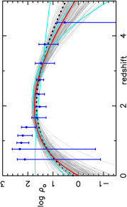
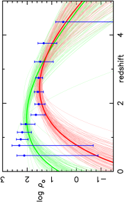
We then used this simple formulation of the evolution function as follows – ascribe zero evolution ($k=0.0$) across individual narrow redshifts slices, adopt a (best) single-valued power law for the luminosity function ($\alpha=2.5$), and calculate the maximum-likelihood value of $\rho_{0}$, the normalization of this luminosity function in each slice. The results should roughly map space density with epoch, and are shown in Fig. 3.

Figure 3: Relative space density in successive redshift slices of width $\Delta\log z=0.7$, incrementing each bin mid-point by $0.25$ in $\log z$ (see the text). Error bars are derived from $\sqrt{N}$, with $N$ the number of objects per bin. The red curve is a maximum-likelihood functional fit to all the data. Grey lines represent 100 bootstrap trials of the evolution model, with bootstrapping end-to-end from the initial sample of 35 SMGs. The three light blue curves represent exponential cut-off models (described in the text); the uppermost corresponds to $n=1$. The dotted line is the result of including the three unidentified sources and ascribing them each a redshift of 4.0 (see the text). Note that the curves are not fits to the points in the diagram – they result from the best likelihood fit to the entire luminosity–redshift plane for the assumed luminosity-function form.

This evolution of the luminosity function with redshift was examined with a simple modification of the previous density evolution: replacing the original power of $(1+z)$, namely $k$, with the modified power $(k+\gamma z)$, i.e.

$$\rho(L,z)=\rho_{o}(1+z)^{(k+\gamma z)}l^{-\alpha}.$$ (8)

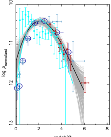
There is as little physical justification for introduction of the $\gamma z$ term in the exponent as there was for the assumption of the initial power law, or for the factorization. However, the term provides a generic description of redshift behaviour – if $\gamma$ is negative, there is a roll-off in density toward higher $z$. The results are again shown in Fig. 3. The red curve is a minimization of the likelihood function $S$ for all three parameters $k$, $\gamma$ and $\alpha$, determined with a downhill simplex routine (Press et al., 1992). The maximum likelihood was found at $k=6.0\pm 2.5$, $\gamma=-1.2\pm 0.4$, and $\alpha=2.5\pm 0.3$ (see Table 1). The curves describe the individual slice normalizations reasonably. The exponent of the initial rise ($k$) is similar to those found in investigations of objects at other frequencies (radio and X-ray AGN; see e.g. Wall et al. 1980); the roll-off shows a maximum space density of the SMGs at about $z=2.0$, in accordance with the appearance of the $L{-}z$ plane (Fig. 1). Fig. 3 includes data from a bootstrap analysis; 100 end-to-end bootstrap results from the original sample of 35 objects are shown. Some 200 were done in all and none produced a value of $\gamma$ approaching zero.

Table 1: Best-fit density evolution parameters.

(Sub) sample‡	$\rho_{0}$/Gpc-3	$\alpha$	$k$	$\gamma$
complete (35)	3490	2.5 (0.3)	6.0 (2.5)	$-1.2$ (0.4)
complete+3* (38)	6334	2.5	4.8	$-0.9$
T${}_{\rm eff}=35\pm 10$K (35)	7685	2.4	4.4	$-0.9$
T${}_{\rm eff}=10(1+z)$K (35)	2956	2.4	5.6	$-1.1$
$z^{\prime}=z\pm 0.14(1+z)$ (35)	14010	2.5	3.7	$-0.8$
low-$L^{\dagger}$ (17)	11970	2.1 (0.8)	5.3 (3.0)	$-1.3$ (0.7)
high-$L^{\dagger}$ (18)	208	3.3 (0.7)	12.3 (6.0)	$-1.8$ (0.7)

^‡Sample/sub-sample number of sources in brackets.                                                 
^∗Total sample, with redshifts of 4.0 assigned to the three unidentified sources.               
^†Two sub-populations, with the sample of 35 divided at the median $850\,\mu$m luminosity,
$\log(L_{850\,\mu{\rm m}}/{\rm W}\,{\rm Hz}^{-1}{\rm sr}^{-1})=23.2$.

A tenet of Bayesian analysis is that all obvious models should be tried. We considered pure luminosity evolution, but on the assumption of a power-law luminosity function, this is identical to density evolution, as shown by Marshall et al. (1983). We checked this by formulating pure luminosity evolution, and derived precisely the same results as for density evolution, the same minimum value of the Likelihood function, and the same parameters, modified by the relations to transcribe density into luminosity evolution given by Marshall et al. (1983). Other forms of the redshift cut-off were tried, in particular an exponential roll-off:

$$\rho(L,z)=\rho_{o}(1+z)^{k}\exp[-(z/z_{*})^{n}]l^{-\alpha}.$$ (9)

The best fit for $n\,{=}\,1$ (Fig. 3, light blue lines) gives a minimum likelihood markedly larger than that for the original form, while the best fits for $n\,{=}\,2$ and $n\,{=}\,3$ are close in minimum likelihood value to the best fit for the original form. Fig. 3 shows why – these latter two forms are very similar, and are encompassed by the bootstrap results. Note, however, that these forms of roll-off introduce a fourth parameter.

To consider how the three missing redshifts in the total sample of 38 objects might affect the reality of the cut-off, we adopted a conservative position: we ascribed a redshift of 4.0 to each of the three unidentified sources in the total sample of 38 objects. Running the minimization procedure for all 38 produced (Table 1; sample ‘complete+3’) the result shown as the dotted line in Fig. 3. It is encompassed by the bootstrap trials; the missing redshifts do not change our conclusion. As a further conservative test, we ran the minimization for the 24/35 objects with redshift determinations from spectroscopy or other optical data. The resulting parameters do not differ significantly from those for the sample of 35 objects; the cut-off is secure.

There are two obvious ways in which our assumption of a single equivalent temperature of 35K could be in error, a serious concern because of our choice of rest-frame $850\,\mu$m as the luminosity measure. One is that there might be significant scatter about this temperature. We tested the effect of this by a simulation in which we adopted a Gaussian spread about 35K of $\sigma=10$K; our particular simulation for the 35 objects yielded a maximum temperature of 59.6K and a minimum of 15.4K. The resulting parameters are given in Table 1. They are encompassed within the errors for the complete sample. A second way in which the equivalent temperature could differ from our single adopted value is a dependence on redshift. We tried a dependence of the form $T(z)=10(1+z)\ K$ (Kovács et al., 2006), and the parameters resulting (Table 1) were again unchanged within the uncertainties. It thus appears that we are viewing predominantly density or luminosity evolution rather than spectral evolution.

Figure 4: Contours of probability for marginalized parameters of equation 8. The contours are linearly spaced, with green contours representing 68 and 95 per cent regions, respectively (corresponding to 1 and $2\sigma$, but for two-dimensional data). Green crosses show the optimum values as determined by the downhill simplex minimization, while blue crosses represent the marginalized contour minima. The 200 bootstrap results are plotted as dots. Note the ‘zones of avoidance’ of the bootstrap results, particularly in the central panel. This is discussed in §5.

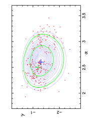
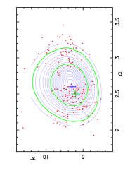
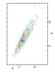
The interplay between the parameters ($\alpha,k,\gamma$) can best be seen by marginalization over each of them in turn, a process to examine degeneracies. Fig. 4 shows the marginalized posterior probability density functions for pairs of the 3 parameters, assuming flat priors. The only degeneracy is the one anticipated – large values of $k$ (steep initial evolution) require correspondingly large negative values of $\gamma$ to ‘restore’ the space density to its observed low values at high redshifts. There is no significant dependence of the slope of the luminosity function on the evolution parameters. Marginalizing over all parameters to find the probability distribution of $\gamma$ gives a clear indication of the need for a redshift cut-off to describe the data. This probability distribution is shown in Fig. 5.

Figure 5: The probability distribution for parameter $\gamma$, which describes the deviation from redshift power-law evolution through $(1+z)^{k+\gamma z}$. If $\gamma$ is negative a redshift cut-off is implied, as the $\gamma z$ term of the exponent must overpower $k$ at redshifts somewhat greater than $z=-k/\gamma$.

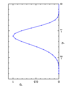
It indicates that there is essentially no probability of $\gamma$ being positive – the data demand a formulation of the evolving luminosity function which specifies a redshift cut-off. For this model the significance of $\gamma\geq 0$ is too small to measure.

Fig. 6 shows a comparison of the epoch behaviour of the luminosity function with the space-density dependence established for QSOs selected in different wavebands. The coincidence in form is remarkable, and is discussed further in §6.

Figure 6: The data of Fig. 3 (light blue) superposed on a compilation (see Wall et al. 2005) of QSO space-density dependences on redshift. The compilation includes QSOs which are selected optically (red triangles: Sloan Digital Sky Survey, Schmidt et al. 1995; Fan et al. 2001, 2004), in X-ray bands (blue circles and crosses, Hasinger et al. 2005; Hasinger 2005; Silverman et al. 2005) and from radio surveys (grey shading, black line, Wall et al. 2005).

The bootstrap results in this analysis indicate broad agreement with the simple adopted model, but do not inspire confidence in either the model details or the parameters derived from it. The bootstrap parameter distributions are non-Gaussian and show zones of avoidance, particularly in the upper and middle panels of Fig. 4. We return to this issue in §5.

4 The star formation rate

From the spectral assumptions of a greybody with $\beta=1.5$ and $T=35\,$K, we calculated the total IR luminosity and converted it to star formation rate for each galaxy using the relationship for starburst galaxies given by Kennicutt (1998). This ‘cold-dust’ SFR assumes a Salpeter (1955) initial mass function and applies to starbursts with ages less than $100\,$Myr. It also assumes little or no AGN contribution to the IR luminosity, a reasonably good assumption for SMGs (Alexander et al., 2005; Pope et al., 2006). Furthermore, since we have assumed only a greybody template with one temperature, we are not including any contribution of warm dust and/or mid-IR spectral features to the IR luminosity – the values we use here are for the cold dust only, which is expected to dominate in such systems (Pope et al., 2006; Huynh et al., 2006). Because of these and other systematic effects, our results will be difficult to compare in detail with SFRD derived from samples selected in other wavebands. Nevertheless, the results should give reasonable estimates for SFRD evolution, provided that the dust properties do not vary appreciably with redshift.

Dividing space up into redshift shells, the volume contribution for each galaxy was calculated from $\Delta V=V_{\rm max}-V_{\rm min}$, where $V_{\rm min}$ is the lower redshift limit of the shell, and $V_{\rm max}$ is either the shell upper redshift limit or the $V_{\rm max}$ value determined from the redshift at which the galaxy encounters its individual survey limit line (Fig. 1) – whichever is smaller. Each galaxy then makes a contribution to the SFRD in the shell of $({\rm SFR}_{i}/\Delta V_{i})\times(4\pi/A_{i})$ where $A_{i}$ is the area of each ‘single-source-survey’, as described earlier. The result of such a calculation for redshift shells of $\Delta z=0.6$ is shown in Fig. 7 – of course the results are not very different from a scaled version of Fig. 3.

Figure 7: Star formation rate density as a function of redshift, in redshift shells $\Delta z=0.6$.

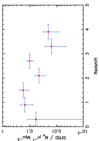
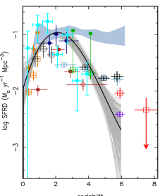
Although these estimates are noisy, there is evidence from the plot that the SFRD from SMGs declines at redshifts beyond three. Fig. 8 shows the points of Fig. 7 in comparison with numerous other recent estimates of the epoch dependence of star formation rate density.

Figure 8: The data of Fig. 7 (light blue) superposed on a compilation of SFRD estimates as a function of redshift; see Wall et al. (2005) for details. The black line and grey shading represents the space distribution of radio QSOs, from Fig. 6, arbitrarily scaled. The dark red circles (Chapman et al., 2005) represent perhaps the most important comparison; these are estimates from a sample of radio-detected, spectroscopically-confirmed SMGs, but are not an unbiased sample as represented by the present data.

5 Two populations?

The unsatisfactory bootstrap results shown in Fig. 4 suggest non-Gaussianity and more specifically a dichotomy, indicating that we may be looking at two populations.

We originally suspected this feature of the population to be due to sample problems, from errors in redshift estimates, errors in identifications, or to a unique distribution of luminosities whose analysis would be fragile in the face of errors in the identification process. We therefore tested for robustness in a number of different ways.

We first considered errors in the redshift estimates. Assuming the spectroscopic redshifts to be correct, we ran many realizations of our sample with the photometric redshifts randomly dispersed about the measured values, applying Gaussian errors of $\Delta z=0.14(1+z)$, twice the size of the error estimated in these redshifts by Pope et al. (2006). The bootstrap tests always yielded plots of similar appearance, with a bifurcated spread of points. We then dropped the assumption that the spectroscopic redshifts were correct, and repeated the exercise for all objects in the sample. The parameter set for the first of these realizations is in Table 1, its values encompassed again by the spread in values from the original sample. The results persisted, the same bifurcated spread of points appearing. Thus the bootstrap structure does not appear to be the result of ‘preferred’ redshift estimates.

We modelled errors in identifications in two ways. First we reduced the sample by randomly throwing out ‘misidentifications’, creating sample realizations by removing one, two or three objects at random in the following sequence. For one object, a single SMG was removed from the set of 12 less secure identifications; for two objects, one was removed from the 23 secure identifications and one from the 12 less secure; for three objects, two were removed from the less secure identifications and one from the secure identifications. Three errors in identifications is the maximum number we would anticipate, based on the summed probabilities of identification reliabilities.

Secondly we retained the sample size and mimicked the possibility of misidentifications as follows. We assumed that the redshift distribution is correct; this is a reasonable approximation, as the great majority of sample members are correctly identified and there is no identifiable bias in the redshift determinations. We then assumed one, two or three objects at random were misidentified, following the foregoing choice sequence amongst the secure and less secure identifications. We assigned a new redshift to each of these one, two or three objects, drawn at random from the distribution of all redshifts in the sample.

A maximum of three identification errors might be realistically expected from the summed identification probabilities. To be extreme (and unrealistic), we tried simulations in which up to 8 of the identifications were deemed incorrect.

None of these realizations destroyed the general appearance of the bootstrap results shown in Fig. 4. In some cases the zone of avoidance was less well defined; but all showed the same relatively tight clustering of points to the left of the contour maximum, and a rather more diffuse distribution of points to the right (upper two panels, Fig. 4). In no case did the general appearance of ‘two clumps’ disappear.

Although this was equally true for the realizations involving excess redshift errors, in these cases the errors had the effect of reducing the evolution parameter $k$ (Table 1), shifting the distribution downward in the central panel of Fig. 4. This is understandable in that adding noise to the redshift distribution (see Fig. 1) will reduce the sharpness of the ‘rise’ towards $z=1$ and make the fall-off after $z=4$ somewhat more gentle. The effect is equivalent to broadening the distribution of luminosities in the complete sample. Less space-density evolution will be required. Placing a scatter on the equivalent temperature produces the same broadening of the luminosity distribution, and again the lower value of the evolution exponent is evident in Table 1.

A bifurcated spread of points as a stable feature of the sample suggested that the data have something more to tell us.

To examine this, we divided the sample of 35 at the median luminosity of log $L_{850\mu m}=23.2$ and repeated the likelihood analysis for each subsample. The minimization routine yielded the results set out once more in Table 1.

The differences between the parameters for the subsamples now strongly suggest the presence of two distinct populations. Although the individual parameters do not differ at high significance levels, the joint probabilities show the subsamples occupying distinct and markedly different regions of the 3D parameter space. The lower-luminosity objects show a luminosity function of slope around $-2$ and relatively mild cosmic evolution, $k\sim 5$. The slope of the luminosity function for the more luminous objects is closer to $-3$ and the evolution is much more dramatic, with $k\sim 14$. In both subsamples, the value of $\gamma$, the redshift cut-off parameter, is significantly below zero; the data support a redshift cut-off for each subsample.

A global minimization solution of the likelihood function for two sub-populations yielded essentially identical results. In this test each sub-population was required to have independent evolution described by the three parameters, with the dividing luminosity set as a seventh free parameter. The key point from this analysis is that the luminosity split between the sub-populations emerged as identical (to 1 decimal place in the log) to the log median adopted a priori.

The previous probability analyses with marginalizations were then carried through for the two subsamples individually. The structure of the points in Fig. 3 (reproduced in Fig. 9) is better represented by the two-component luminosity function, as Fig. 9 demonstrates.

Figure 9: The points and error bars are the data described and presented in Fig. 3. The green curve is a functional fit to the low-luminosity data using maximum likelihood with a minimization routine, and faint green lines represent 100 bootstrap trials of the evolution model, with bootstrapping end-to-end from this subsample of 17 SMGs. The red curve and its faint red counterparts are the best fit and bootstrap fits for the 18 higher-luminosity objects. The sum of the two components is a reasonable representation of the form of the successive redshift-slice values of $\rho_{0}$.

The three diagrams of Fig. 4 now become 6 diagrams; as representatives, Fig. 10 gives the two separate $k-\alpha$ plots, the plane (middle panel, Fig. 4) which previously showed the least satisfactory distribution of bootstrap points. The bootstrap points in these two plots are now distributed as expected, suggesting Gaussianity prevails for each sub-sample.

Figure 10: Contours of probability for marginalized parameters $k$ (evolution as $(1+z)^{k}$) and $\alpha$ ($-$slope of the power-law luminosity function): top, low-luminosity subsample; bottom, high-luminosity subsample. The plots are on the same axes to demonstrate that the preferred regions hardly intersect, i.e. both parameters differ between the two subsamples. As before the contours are linearly spaced: green contours represent 68 per cent and 95 per cent regions, respectively. The distributions of the bootstrap points are now approximately Gaussian in appearance; in each case $68\pm 2$ out of the 100 points fall within the effectively $1\sigma$ contours.

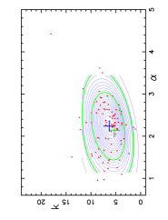
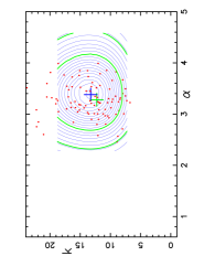
To demonstrate the significance of the difference between the two sub-populations, we computed the value of the likelihood function for each subsample using the maximum-likelihood parametric fit obtained for the other subsample. We then compared this value with the maximum-likelihood value found for the subsample. The respective differences for the low-luminosity sample and the high-luminosity sample were 25.6 and 19.0 in $\chi^{2}$ for 3 degrees of freedom. This indicates rejection of the model for each subsample by the data of the other subsample, at the $\leq 0.001$ level of significance. In addition we ran 1000 bootstrap tests on each subsample to find how frequently the resultant model parameters overlapped those determined from the maximum-likelihood solution for other subsample. Considering for example the high-luminosity sample bootstraps, how many times out of 1000 would we find (see Table 1) $\alpha\leq 2.1,k\leq 5.3$ and $\gamma\geq-1.3$? In fact we found $0/1000$, and for the low-luminosity sample we found $3/1000$. This test again indicates a difference between the subsample models at a significance level of about $0.001$. (Note that these tests are valid only because we split our sample into high and low-luminosity subsamples a priori, i.e. without optimization.)

The single-dimensional distribution of SMG luminosities shows no strong indication of a dichotomy. However, this is not an argument against the presence of two populations; samples of 100s of radio sources likewise show no clear dichotomy in the luminosity distribution, despite the known presence of low-luminosity and high-luminosity populations, largely distinct in morphology and evolving very differently (Dunlop & Peacock, 1990; Jackson & Wall, 1999; Sadler et al., 2007). Beyond the inevitable correlations of flux and luminosity with redshift, Pope et al. (2006) found no additional correlations of spectral properties with redshift.

We conclude that statistically the two-population hypothesis is solidly based. However we cannot deny that the sample is small, with the remote possibility of a unique assemblage of objects leading us astray.

Finally, we carried out the SFR calculation individually for the two subsamples. The procedure as described in §4 was followed, with the results appearing in Fig. 11.

Figure 11: Star formation rate density as a function of redshift, using redshift shells $\Delta z=0.6$: left-hand panel, low-luminosity SMG subsample; right-hand panel, high-luminosity SMG subsample.

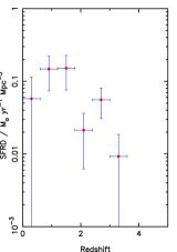
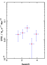
The diagram shows that the star-formation rate dependence on epoch differs for the two sub-populations, the SFRD peaking around $z\sim 1.5$ for the lower luminosities and around $z\sim 2.5$ for the higher luminosities. Of course this result is not at all independent of the different forms of SMG volume-density evolution found for the two subsamples (Table 1 and Fig. 9).

6 Discussion and Conclusions

We have shown that there is a significant decline in the space density of SMGs beyond a redshift of three. This conclusion has undergone extensive testing via bootstrap analyses plus the investigation of different forms for the evolution.

Several authors (e.g. Sanders et al., 1988; Genzel et al., 1998; Archibald et al., 2002; Stevens et al., 2005; Di Matteo et al., 2005; Alexander et al., 2005) have suggested a connection between the formation of powerful QSOs and ULIRGs (or their high-$z$ counterparts the SMGs). A popular picture has emerged of an evolutionary sequence in which the forming galaxy is initially far-IR luminous but X-ray weak, similar to the sources discovered as SMGs. As the black hole and spheroid grow with time, a point is reached when the central QSO becomes powerful enough to terminate the star formation and eject the bulk of the fuel supply. This transition is followed by a period of unobscured QSO activity, subsequently declining to leave a quiescent spheroidal galaxy. For the first time (Fig. 6) we have been able to compare the space densities of QSOs and SMGs. Such a scenario is consistent with our results, in which we find remarkable concordance between the space density decline shown by the SMGs, by all types of QSOs and by the SFRD from SMGs. Examining the significance of the time sequence is beyond the capabilities of the present data, but at a minimum the data emphasize the strong connection between SMGs, AGN activity and cold-dust SFRD.

The cold-dust-derived SFRD from SMGs shows a significant decline at redshifts beyond about three. The larger star-formation rate from the more distant and higher-luminosity objects is inadequate to overcome the rapid decline in their volume density. If there is significant star formation beyond redshifts of 4, it is not the province of SMGs, but must be carried by different and generally lower-luminosity populations, such as the Lyman-break galaxies (Steidel et al., 1999) or galaxies found in very deep searches at optical wavelengths (Bouwens et al., 2004; Giavalisco et al., 2004). Semi-analytic modelling of the SFRD from SMGs (e.g. Baugh et al., 2005) suggests a broad peak at $2<z<3$, although the predicted diminution to higher redshifts is less than that indicated by the results here.

There is evidence suggesting that the submm population may be strongly clustered (e.g. Blain et al., 2004). Although our results are based on submm observations in a small field, we note that our main conclusions will be unaffected by clustering unless the clustering strength of SMGs depends strongly on their luminosity. However, the redshifts of the sample members are so large and so diverse that there is no possibility of sample members occupying the same supercluster or filament. There is thus little likelihood that cosmic variance is affecting the results.

The data are remarkably insistent on the presence of two subpopulations of objects, divided by luminosity. These evolve in distinctly different ways and their luminosity functions have different shapes. Their SFRD histories are likewise very different. The ULIRG/LIRG dichotomy is of particular relevance here, and our results are similar to those discussed in some earlier studies of lower redshift populations (e.g. Kim & Sanders, 1998; Guiderdoni et al., 1998; Chary & Elbaz, 2001; Lagache et al., 2003; Sajina et al., 2003; Xu et al., 2003), sometimes more loosely described as a distinction between ‘starbursts’ versus more normal galaxies. At higher redshifts Chary (2006) illustrated (in his fig. 4) how SFRD dominance shifts from ULIRGs at $z\geq 2.5$ to LIRGs at $z\sim 1$ (see also Caputi et al. 2007 and other Spitzer-based studies). Our dividing line in luminosity is somewhat more extreme than the LIRG/ULIRG boundary, normally taken at $10^{12}{\rm L}_{\odot}$; our division at $\log L_{850\mu\rm{m}}=23.2$ corresponds to about $3\times 10^{12}{\rm L}_{\odot}$. Despite our higher adopted dividing line, our results parallel those for LIRGs/ULIRGS: we find the most IR-luminous SMGs dominating the energy output (or SFRD) at $z\sim 2.5$, while the less luminous SMGs dominate the SFRD at $z\sim 1$. Note that this analysis does account for the contribution to the SFRD from high redshift LIRGs and ULIRGs selected at shorter IR or radio wavelengths. Within the submm population, we are seeing a down-sizing in the luminosity of the dominant contributors to the energy budget.

We conclude that a redshift cut-off is established for SMGs in both object density and SFRD, both of which are similar in form to cut-offs found for powerful AGN. The redshift cut-off is established with such certainty that that for the models adopted, the level of significance is too small to calculate. We also conclude that at a level of significance of $\sim 0.001$, two populations are probably present amongst SCUBA-detected SMGs, showing distinctly different evolutionary histories and luminosity functions. Although cosmic dowsizing is certainly present, we note that our sample is small; and despite extensive testing, the two-population hypothesis could have resulted from a singular grouping of data. However, we can be optimistic that with much larger samples soon to be collected using SCUBA-2 (Holland et al., 2006), it will be possible to test the several ideas and issues which arise from our study. These include: further probing of the two population question; the AGN–SFR connection and its time-lag; the role merging plays in this process; details of how and why SMGs possibly organize themselves to manifest cosmic down-sizing; and the relation this down-sizing has to populations of LIRGs and ULIRGs selected at other wavelengths.

Acknowledgements. We are very grateful to Chris Blake for many helpful discussions and suggestions, and to Mitch Crowe for work on including additional ‘two bolometer chopping’ SCUBA data in the supermap. Helpful comments from a referee resulted in a significantly improved manuscript. This work was supported by the Natural Sciences and Engineering Research Council of Canada and by the Canadian Space Agency.

Appendix A Data for the three additional sources of the sample

Table 2: The three new GOODS-N supermap sources.

Submm ID	Submm name	Radio RA	Radio Dec	Raw S850 (mJy)	Deboosted S850 (mJy)	Redshift	P
GN39	SMMJ123711.1+621325	12:37:11.33	62:13:31.02	7.4$\pm$1.9	5.2$\pm$2.4	1.996	0.02
		12:37:11.97	62:13:25.77
GN40	SMMJ123713.7+621822	12:37:13.86	62:18:26.24	13.1$\pm$2.7	10.7$\pm$2.9	2.6	0.003
GN41	SMMJ123639.4+620752	n/a	n/a	11.9$\pm$3.1	8.8$\pm$3.5

Table 2 gives positions, fluxes and redshifts of the three new GOODS-N supermap sources. The submm name gives the position of the submm source while RA and Dec provide the position of the radio counterpart. The counterpart identifications were performed exactly as outlined by Pope et al. (2006). We list both the raw and deboosted submm fluxes. $P$ is the probability that the counterpart is a random association [see Pope et al. (2006) for more details on these probabilities]. GN39 appears in the Chapman et al. (2005) catalogue and has two radio counterparts, both confirmed to lie at the same redshift (Swinbank et al., 2004; Chapman et al., 2005); we list the two radio positions. The redshift of GN40 is an IRAC-only photometric redshift as described by Pope et al. (2006). GN41 does not have a unique likely counterpart and is therefore not included in the analysis of this paper.

References

- Alexander et al. (2005) Alexander D. M., Bauer F. E., Chapman S. C., Smail I., Blain A. W., Brandt W. N., Ivison R. J., 2005, Astrophys. J., 632, 736
- Alexander et al. (2005) Alexander D. M., Smail I., Bauer F. E., Chapman S. C., Blain A. W., Brandt W. N., Ivison R. J., 2005, Nature, 434, 738
- Archibald et al. (2002) Archibald E. N., Dunlop J. S., Jimenez R., Friaça A. C. S., McLure R. J., Hughes D. H., 2002, Mon. Not. R. astr. Soc., 336, 353
- Baugh et al. (2005) Baugh C. M., Lacey C. G., Frenk C. S., Granato G. L., Silva L., Bressan A., Benson A. J., Cole S., 2005, Mon. Not. R. astr. Soc., 356, 1191
- Blain et al. (2004) Blain A. W., Chapman S. C., Smail I., Ivison R., 2004, Astrophys. J., 611, 725
- Blain & Longair (1993) Blain A. W., Longair M. S., 1993, Mon. Not. R. astr. Soc., 264, 509
- Blain et al. (2002) Blain A. W., Smail I., Ivison R. J., Kneib J.-P., Frayer D. T., 2002, Phys. Rep., 369, 111
- Blake et al. (2006) Blake C., Pope A., Scott D., Mobasher B., 2006, Mon. Not. R. astr. Soc., 368, 732
- Borys et al. (2003) Borys C., Chapman S., Halpern M., Scott D., 2003, Mon. Not. R. astr. Soc., 344, 385
- Bouwens et al. (2004) Bouwens R. J. et al., 2004, Astrophys. J. Lett., 616, L79
- Caputi et al. (2007) Caputi K. I., Lagache G., Yan Lin, Dole H., Bavouzet N., Le Floc’h E., Choi P. I., Helou G., Reddy N., 2007, Astrophys. J., 660, 97
- Chapman et al. (2005) Chapman S. C., Blain A. W., Smail I., Ivison R. J., 2005, Astrophys. J., 622, 772
- Chary & Elbaz (2001) Chary R., Elbaz D., 2001, Astrophys. J., 556, 562
- Chary (2006) Chary R.-R., 2006, astro-ph/0612736
- Coppin et al. (2005) Coppin K., Halpern M., Scott D., Borys C., Chapman S., 2005, Mon. Not. R. astr. Soc., 357, 1022
- Cowie et al. (1996) Cowie L. L., Songaila A., Hu E. M., Cohen J. G., 1996, Astron. J., 112, 839
- Di Matteo et al. (2005) Di Matteo T., Springel V., Hernquist L., 2005, Nature, 433, 604
- Dunlop & Peacock (1990) Dunlop J. S., Peacock J. A., 1990, Mon. Not. R. astr. Soc., 247, 19
- Fan et al. (2001) Fan X. et al., 2001, Astron. J., 121, 54
- Fan et al. (2004) Fan X. et al., 2004, Astron. J., 128, 515
- Genzel et al. (1998) Genzel R. et al., 1998, Astrophys. J., 498, 579
- Giavalisco et al. (2004) Giavalisco M. et al., 2004, Astrophys. J. Lett., 600, L103
- Guiderdoni et al. (1998) Guiderdoni B., Hivon E., Bouchet F. R., Maffei B., 1998, Mon. Not. R. astr. Soc., 295, 877
- Hasinger (2005) Hasinger G., 2005, in Merloni A., Nayakshin S., Sunyaev R. A., eds, Growing Black Holes: Accretion in a Cosmological Context, Springer: Berlin, p. 418
- Hasinger et al. (2005) Hasinger G., Miyaji T., Schmidt M., 2005, Astron. Astrophys., 441, 417
- Holland et al. (1999) Holland W. S. et al., 1999, Mon. Not. R. astr. Soc., 303, 659
- Holland et al. (2006) Holland W. et al., 2006, Proc. SPIE, 6275, 62751E
- Hughes et al. (1998) Hughes D. H. et al., 1998, Nature, 394, 241
- Huynh et al. (2006) Huynh M. T., Pope A., Frayer D. T., Scott D., 2006, Astrophys. J., 659, 305
- Jackson & Wall (1999) Jackson C., Wall J., 1999, Mon. Not. R. astr. Soc., 304, 160
- Kennicutt (1998) Kennicutt Jr. R. C., 1998, ARA&A, 36, 189
- Kim & Sanders (1998) Kim D.-C., Sanders D. B., 1998, Astrophys. J. Suppl., 119, 41
- Kovács et al. (2006) Kovács A., Chapman S. C., Dowell C. D., Blain A. W., Ivison R. J., Smail I., Phillips T. G., 2006, Astrophys. J., 650, 592
- Lagache et al. (2003) Lagache G., Dole H., Puget J.-L., 2003, Mon. Not. R. astr. Soc., 338, 555
- Le Floc’h et al. (2005) Le Floc’h E. et al., 2005, Astrophys. J., 632, 169
- Lilly et al. (1999) Lilly S. J., Eales S. A., Gear W. K. P., Hammer F., Le Fèvre O., Crampton D., Bond J. R., Dunne L., 1999, Astrophys. J., 518, 641
- Longair (1966) Longair M. S., 1966, Mon. Not. R. astr. Soc., 133, 421
- Marshall et al. (1983) Marshall H. L., Tananbaum H., Avni Y., Zamorani G., 1983, Astrophys. J., 269, 35
- Pérez-González et al. (2005) Pérez-González P. G. et al., 2005, Astrophys. J., 630, 82
- Pope (2007) Pope A., 2007, PhD thesis, University of British Columbia
- Pope et al. (2005) Pope A., Borys C., Scott D., Conselice C., Dickinson M., Mobasher B., 2005, Mon. Not. R. astr. Soc., 358, 149
- Pope et al. (2006) Pope A. et al., 2006, Mon. Not. R. astr. Soc., 370, 1185
- Press et al. (1992) Press W. H., Teukolsky S. A., Vetterling W. T., Flannery B. P., 1992, Numerical recipes in FORTRAN. CUP, 1992, 2nd ed.
- Sadler et al. (2007) Sadler E. M. et al., 2007, Mon. Not. R. astr. Soc., 381, 211
- Sajina et al. (2003) Sajina A., Borys C., Chapman S., Dole H., Halpern M., Lagache G., Puget J.-L., Scott D., 2003, Mon. Not. R. astr. Soc., 343, 1365
- Salpeter (1955) Salpeter E. E., 1955, Astrophys. J., 121, 161
- Sanders & Mirabel (1996) Sanders D. B., Mirabel I. F., 1996, ARA&A, 34, 749
- Sanders et al. (1988) Sanders D. B., Soifer B. T., Elias J. H., Neugebauer G., Matthews K., 1988, Astrophys. J. Lett., 328, L35
- Schmidt et al. (1995) Schmidt M., Schneider D. P., Gunn J. E., 1995, Astron. J., 110, 68
- Silverman et al. (2005) Silverman J. D. et al., 2005, Astrophys. J., 624, 630
- Steidel et al. (1999) Steidel C. C., Adelberger K. L., Giavalisco M., Dickinson M., Pettini M., 1999, Astrophys. J., 519, 1
- Stevens et al. (2005) Stevens J. A., Page M. J., Ivison R. J., Carrera F. J., Mittaz J. P. D., Smail I., McHardy I. M., 2005, Mon. Not. R. astr. Soc., 360, 610
- Swinbank et al. (2004) Swinbank A. M., Smail I., Chapman S. C., Blain A. W., Ivison R. J., Keel W. C., 2004, Astrophys. J., 617, 64
- Ueda et al. (2003) Ueda Y., Akiyama M., Ohta K., Miyaji T., 2003, Astrophys. J., 598, 886
- Wall et al. (2005) Wall J. V., Jackson C. A., Shaver P. A., Hook I. M., Kellermann K. I., 2005, Astron. Astrophys., 434, 133
- Wall et al. (1980) Wall J. V., Pearson T. J., Longair M. S., 1980, Mon. Not. R. astr. Soc., 193, 683
- Xu et al. (2003) Xu C. K., Lonsdale C. J., Shupe D. L., Franceschini A., Martin C., Schiminovich D., 2003, Astrophys. J., 587, 90