New Inflation vs. Chaotic Inflation, higher degree potentials and the Reconstruction Program in light of WMAP3

D. Boyanovsky boyan@pitt.edu Department of Physics and Astronomy, University of Pittsburgh, Pittsburgh, Pennsylvania 15260, USA Observatoire de Paris, LERMA. Laboratoire Associé au CNRS UMR 8112.
61, Avenue de l’Observatoire, 75014 Paris, France.
LPTHE, Université Pierre et Marie Curie (Paris VI) et Denis Diderot (Paris VII), Laboratoire Associé au CNRS UMR 7589, Tour 24, 5ème. étage, 4, Place Jussieu, 75252 Paris, Cedex 05, France
   H. J. de Vega devega@lpthe.jussieu.fr LPTHE, Université Pierre et Marie Curie (Paris VI) et Denis Diderot (Paris VII), Laboratoire Associé au CNRS UMR 7589, Tour 24, 5ème. étage, 4, Place Jussieu, 75252 Paris, Cedex 05, France Observatoire de Paris, LERMA. Laboratoire Associé au CNRS UMR 8112.
61, Avenue de l’Observatoire, 75014 Paris, France.
Department of Physics and Astronomy, University of Pittsburgh, Pittsburgh, Pennsylvania 15260, USA
   C. M. Ho cmho@phyast.pitt.edu Department of Physics and Astronomy, University of Pittsburgh, Pittsburgh, Pennsylvania 15260, USA    N. G. Sanchez Norma.Sanchez@obspm.fr Observatoire de Paris, LERMA. Laboratoire Associé au CNRS UMR 8112.
61, Avenue de l’Observatoire, 75014 Paris, France.
Abstract

The CMB power spectra are studied for different families of single field new and chaotic inflation models in the effective field theory approach to inflation. We implement a systematic expansion in 1/Ne1subscript𝑁𝑒1/N_{e} where Ne50similar-tosubscript𝑁𝑒50N_{e}\sim 50 is the number of e-folds before the end of inflation. We study the dependence of the observables (ns,rsubscript𝑛𝑠𝑟n_{s},\;r and dns/dlnk𝑑subscript𝑛𝑠𝑑𝑘dn_{s}/d\ln k) on the degree of the potential (2n2𝑛2\,n) and confront them to the WMAP3 and large scale structure data: This shows in general that fourth degree potentials (n=2𝑛2n=2) provide the best fit to the data; the window of consistency with the WMAP3 and LSS data narrows for growing n𝑛n. New inflation yields a good fit to the r𝑟r and nssubscript𝑛𝑠n_{s} data in a wide range of field and parameter space. Small field inflation yields r<0.16𝑟0.16r<0.16 while large field inflation yields r>0.16𝑟0.16r>0.16 (for Ne=50subscript𝑁𝑒50N_{e}=50). All members of the new inflation family predict a small but negative running 4(n+1)×104dns/dlnk2×1044𝑛1superscript104𝑑subscript𝑛𝑠𝑑𝑘2superscript104-4\,(n+1)\times 10^{-4}\leq dn_{s}/d\ln k\leq-2\times 10^{-4}. (The values of r,ns,dns/dlnk𝑟subscript𝑛𝑠𝑑subscript𝑛𝑠𝑑𝑘r,\;n_{s},\;dn_{s}/d\ln k for arbitrary Nesubscript𝑁𝑒N_{e} follow by a simple rescaling from the Ne=50subscript𝑁𝑒50N_{e}=50 values). A reconstruction program is carried out suggesting quite generally that for nssubscript𝑛𝑠n_{s} consistent with the WMAP3 and LSS data and r<0.1𝑟0.1r<0.1 the symmetry breaking scale for new inflation is |ϕ0|10MPlsimilar-tosubscriptitalic-ϕ010subscript𝑀𝑃𝑙|\phi_{0}|\sim 10~{}M_{Pl} while the field scale at Hubble crossing is |ϕc|MPlsimilar-tosubscriptitalic-ϕ𝑐subscript𝑀𝑃𝑙|\phi_{c}|\sim M_{Pl}. The family of chaotic models feature r0.16𝑟0.16r\geq 0.16 (for Ne=50subscript𝑁𝑒50N_{e}=50) and only a restricted subset of chaotic models are consistent with the combined WMAP3 bounds on r,ns,dns/dlnk𝑟subscript𝑛𝑠𝑑subscript𝑛𝑠𝑑𝑘r,\;n_{s},\;dn_{s}/d\ln k with a narrow window in field amplitude around |ϕc|15MPlsimilar-tosubscriptitalic-ϕ𝑐15subscript𝑀𝑃𝑙|\phi_{c}|\sim 15~{}M_{Pl}. We conclude that a measurement of r<0.16𝑟0.16r<0.16 (for Ne=50subscript𝑁𝑒50N_{e}=50) distinctly rules out a large class of chaotic scenarios and favors small field new inflationary models. As a general consequence, new inflation emerges more favoured than chaotic inflation.

pacs:
98.80.Cq,05.10.Cc,11.10.-z

I Introduction

Inflation provides a simple and robust mechanism to solve several outstanding problems of the standard Big Bang model infla ; libros becoming a leading paradigm in cosmology. Superhorizon quantum fluctuations amplified during inflation provide an explanation of the origin of the temperature anisotropies in the cosmic microwave background (CMB) and the seeds for large scale structure formationfluc , as well as of tensor perturbations (primordial gravitational waves). Although there is a diversity of inflationary models, most of them predict fairly generic features: a gaussian, nearly scale invariant spectrum of (mostly) adiabatic scalar and tensor primordial fluctuations fluc . These features provide an excellent fit to the highly precise data provided by the Wilkinson Microwave Anisotropy Probe (WMAP) WMAPa ; peiris ; WMAP3 ; WMAP3b which begins to constrain inflationary models.

The combination of CMB peiris ; WMAP3 and large scale structure data SDSS ; 2dF yield fairly tight constraints for the two dimensional marginalized contours of the tensor to scalar ratio r𝑟r and the scalar index nssubscript𝑛𝑠n_{s}. While ns=1subscript𝑛𝑠1n_{s}=1 was excluded at the 95%CLpercent95𝐶𝐿95\%CL in 2dF a most notable result that stems from the analysis of WMAP3 data is a confirmation that a scale invariant Harrison-Zeldovich spectrum is excluded at the 3σ3𝜎3\sigma level WMAP3 . A combination of data from WMAP3 and large scale surveys distinctly favor ns<1subscript𝑛𝑠1n_{s}<1 sanchez . These latest bounds on the index of the power spectrum of scalar perturbations, and emerging bounds on the ratio of tensor to scalar fluctuations r𝑟r begin to offer the possibility to discriminate different inflationary models. For example, the third year WMAP data disfavors the predictions for the scalar index and the tensor to scalar ratio from a monomial inflationary potential λϕ4𝜆superscriptitalic-ϕ4\lambda\;\phi^{4} showing them to lie outside the 3σ3𝜎3\sigma contour, but the simple monomial m2ϕ2/2superscript𝑚2superscriptitalic-ϕ22m^{2}\;\phi^{2}/2 yields a good fit to the data WMAP3 and predicts a tensor to scalar ratio r0.16similar-to𝑟0.16r\sim 0.16 within the range of forthcoming CMB observations.

Current and future CMB observations in combination with large scale structure surveys will yield tight constraints on the inflationary models, this motivates the exploration of clear predictions from the models and their confrontation with the data.

In distinction with the approach followed in peiris ; WMAP3 ; hoki or studies of specific modelssalama , or statistical analysis combined with WMAP3 and LSS datakinkol ; fipele , we study the predictions for the power spectra of scalar fluctuations and the tensor to scalar ratio for families of new and chaotic inflationary models in the framework of the method presented in ref.1sN . This method relies on the effective field theory approach combined with a systematic expansion in 1/Ne1subscript𝑁𝑒1/N_{e} where Ne50similar-tosubscript𝑁𝑒50N_{e}\sim 50 is the number of e-folds before the end of inflation. The family of inflationary models that we study is characterized by effective field theories with potentials of the form

V(ϕ)𝑉italic-ϕ\displaystyle V(\phi) =\displaystyle= V012m2ϕ2+λ2nϕ2n,brokensymmetry\displaystyle V_{0}-\frac{1}{2}\;m^{2}\;\phi^{2}+\frac{\lambda}{2\,n}\;\phi^{2\,n}\quad,\quad{\rm broken~{}symmetry} (1)
V(ϕ)𝑉italic-ϕ\displaystyle V(\phi) =\displaystyle= 12m2ϕ2+λ2nϕ2n,unbrokensymmetry,\displaystyle\frac{1}{2}\;m^{2}\;\phi^{2}+\frac{\lambda}{2\,n}\;\phi^{2\,n}\quad,\quad{\rm unbroken~{}symmetry}\;, (2)

with n=2,3,4𝑛234n=2,3,4\cdots. For broken symmetry models with potentials of the form (1) there are two distinct regions: small and large field, corresponding to values of the inflaton field smaller or larger than the symmetry breaking scale respectively.

We implement the systematic expansion in 1/Ne1subscript𝑁𝑒1/N_{e} where Ne50similar-tosubscript𝑁𝑒50N_{e}\sim 50 is the number of e-folds before the end of inflation when wavelengths of cosmological relevance crossed the Hubble radius1sN . The 1/Ne1subscript𝑁𝑒1/N_{e} expansion is a powerful and systematic tool that allows to re-cast the slow roll hierarchy as expansion in powers of 1/Ne1subscript𝑁𝑒1/N_{e} 1sN . This expansion allows us to implement a reconstruction program reco which yields the scale of the inflaton field when modes of cosmological relevance today crossed the Hubble radius during inflation, and in the case of new inflation models also yields the scale of symmetry breaking.

We study the dependence of the observables (ns,rsubscript𝑛𝑠𝑟n_{s},\;r and dns/dlnk𝑑subscript𝑛𝑠𝑑𝑘dn_{s}/d\ln k) on the degree of the inflaton potential (2n2𝑛2\,n) for new and chaotic inflation and confront them with the WMAP3 data. This study shows in general that fourth degree potentials (n=2𝑛2n=2) provide the best fit to the data. We find that new inflation fits the data on an appreciable wider range of the parameters while chaotic inflation does this in a much narrow range. Therefore, amongst the families of inflationary models studied, new inflation emerges as a leading contender in comparison with chaotic inflation. The present analysis confirms the statement that within the framework of effective field theories with polynomial potentials, new inflation is a preferred model reproducing the present data ciri ; pre ; heclast .

Main results of this article:

  • The region in inflaton field space which is consistent with the marginalized WMAP3 data can be explored in an expansion in ns1+2/Nesubscript𝑛𝑠12subscript𝑁𝑒n_{s}-1+2/N_{e}.

  • We find that the point ns=12/Ne=0.96,r=8/Ne=0.16formulae-sequencesubscript𝑛𝑠12subscript𝑁𝑒0.96𝑟8subscript𝑁𝑒0.16n_{s}=1-2/N_{e}=0.96,\;r=8/N_{e}=0.16 which is in the region allowed by the WMAP3 analysisWMAP3 belongs both to new inflation models as a limiting point and to the simple chaotic inflation monomial, m2ϕ2/2superscript𝑚2superscriptitalic-ϕ22m^{2}\,\phi^{2}/2. (i) This point describes a region in field and parameter space that separates small fields from large fields, and (ii) is a degeneracy point for the family of models describing both chaotic and new inflation.

  • For all members n=2, 3, 4,𝑛234n=2,\;3,\;4,... of the new inflation family, the small field region yields r<0.16𝑟0.16r<0.16 while the large field region yields r>0.16𝑟0.16r>0.16. All members of the new inflation family predict a small but negative running:

    4(n+1)×104dns/dlnk2×104.4𝑛1superscript104𝑑subscript𝑛𝑠𝑑𝑘2superscript104-4\;(n+1)\times 10^{-4}\leq dn_{s}/d\ln k\leq-2\times 10^{-4}\;.

    This new inflation family features a large window of consistency with the WMAP and LSS data for n=2𝑛2n=2 that narrows for growing n𝑛n. If forthcoming data on tensor modes pinpoints the tensor to scalar ratio to be r<0.1𝑟0.1r<0.1, we predict that the symmetry breaking scale for these models is ϕ010MPlsimilar-tosubscriptitalic-ϕ010subscript𝑀𝑃𝑙\phi_{0}\sim 10\,M_{Pl} and that the scale of the field at which modes of cosmological relevance today cross the Hubble radius is ϕcMPlsimilar-tosubscriptitalic-ϕ𝑐subscript𝑀𝑃𝑙\phi_{c}\sim M_{Pl}.

  • Chaotic inflationary models all yield a tensor to scalar ratio r0.16𝑟0.16r\geq 0.16, where the minimum value r=0.16𝑟0.16r=0.16 corresponds to small amplitude of the inflaton and coincides with the value obtained from the monomial m2ϕ2/2superscript𝑚2superscriptitalic-ϕ22m^{2}\phi^{2}/2. The combined marginalized data from WMAP3 WMAP3 yields a very small window of field amplitude, around |ϕc|15MPlsimilar-tosubscriptitalic-ϕ𝑐15subscript𝑀𝑃𝑙|\phi_{c}|\sim 15~{}M_{Pl} within which chaotic models are allowed by the data. These regions become progressively smaller for larger n𝑛n. Some small regions in field space consistent with the WMAP3 data feature peaks in the running of the scalar index but in the region consistent with the WMAP3 data in chaotic inflation the running is again negligible (103similar-toabsentsuperscript103\sim 10^{-3}). If future observations determine a tensor to scalar ratio r<0.16𝑟0.16r<0.16, this by itself will rule out a large family of chaotic inflationary models.

II Effective field theory, slow roll and 1/Ne1subscript𝑁𝑒1/N_{e} expansions

In the absence of a fundamental microscopic description of inflation, an effective field theory approach, when combined with the slow roll expansion provides a robust paradigm for inflation with predictive power. The reliability of the effective field theory description hinges on a wide separation between the Hubble and Planck scales, and is validated by the bound from temperature fluctuations H/MPl<105𝐻subscript𝑀𝑃𝑙superscript105H/M_{Pl}<10^{-5} 1sN .

The slow roll expansion relies on the smallness of a hierarchy of the dimensionless ratios libros ; barrow ; reco ,

ϵv=MPl22[V(ϕ)V(ϕ)]2,ηv=MPl2V′′(ϕ)V(ϕ),ξv=MPl4V(ϕ)V′′′(ϕ)V2(ϕ).\epsilon_{v}=\frac{M^{2}_{Pl}}{2}\;\left[\frac{V^{{}^{\prime}}(\phi)}{V(\phi)}\right]^{2}\quad,\quad\eta_{v}=M^{2}_{Pl}\;\frac{V^{{}^{\prime\prime}}(\phi)}{V(\phi)}\quad,\quad\xi_{v}=M^{4}_{Pl}\;\frac{V^{\prime}(\phi)\;V^{{}^{\prime\prime\prime}}(\phi)}{V^{2}(\phi)}\;. (3)

The effective field theory expansion in H/MPl𝐻subscript𝑀𝑃𝑙H/M_{Pl} and the slow roll expansion are independent, the latter can be interpreted as an adiabatic expansion 1sN wherein the derivatives of the inflationary potential are small.

The CMB data is consistently described within the slow roll expansion with inflationary potentials of the form libros ; 1sN

V(ϕ)=M4v(ϕMPl).𝑉italic-ϕsuperscript𝑀4𝑣italic-ϕsubscript𝑀𝑃𝑙V(\phi)=M^{4}\;v\left(\frac{\phi}{M_{Pl}}\right)\;. (4)

Within the slow roll approximation the number of e-folds before the end of inflation for which the value of the field is ϕendsubscriptitalic-ϕ𝑒𝑛𝑑\phi_{end} is given by

N[ϕ(t)]=1MPl2ϕ(t)ϕendV(ϕ)dϕdV𝑑ϕ.𝑁delimited-[]italic-ϕ𝑡1subscriptsuperscript𝑀2𝑃𝑙superscriptsubscriptitalic-ϕ𝑡subscriptitalic-ϕ𝑒𝑛𝑑𝑉italic-ϕ𝑑italic-ϕ𝑑𝑉differential-ditalic-ϕN\left[\phi(t)\right]=-\frac{1}{M^{2}_{Pl}}\int_{\phi(t)}^{\phi_{end}}V(\phi)~{}\frac{d\phi}{dV}~{}d\phi~{}~{}. (5)

It proves convenient to introduce Nesubscript𝑁𝑒N_{e} as the typical number of e-folds before the end of inflation during which cosmologically relevant wavelengths cross the Hubble radius during inflation, and ϕcsubscriptitalic-ϕ𝑐\phi_{c} as the value of the inflaton field corresponding to Nesubscript𝑁𝑒N_{e}

Ne=1MPl2ϕcϕendV(ϕ)dϕdV𝑑ϕ.subscript𝑁𝑒1subscriptsuperscript𝑀2𝑃𝑙superscriptsubscriptsubscriptitalic-ϕ𝑐subscriptitalic-ϕ𝑒𝑛𝑑𝑉italic-ϕ𝑑italic-ϕ𝑑𝑉differential-ditalic-ϕN_{e}=-\frac{1}{M^{2}_{Pl}}\int_{\phi_{c}}^{\phi_{end}}V(\phi)~{}\frac{d\phi}{dV}~{}d\phi\,. (6)

The precise value of Nesubscript𝑁𝑒N_{e} is certainly near Ne=50subscript𝑁𝑒50N_{e}=50 libros ; Ne . We will take the value Ne=50subscript𝑁𝑒50N_{e}=50 as a reference baseline value for numerical analysis, but from the explicit expressions obtained in the systematic 1/Ne1subscript𝑁𝑒1/N_{e} expansion below, it becomes a simple rescaling to obtain results for arbitrary values of Nesubscript𝑁𝑒N_{e} [see eq. (10) below].

The form of the potential eq.(4) and the above definition for the number of e-folds, suggests to introduce the following rescaled field variable 1sN

ϕ=NeMPlχitalic-ϕsubscript𝑁𝑒subscript𝑀𝑃𝑙𝜒\phi=\sqrt{N_{e}}M_{Pl}\,\chi (7)

where the rescaled field χ𝜒\chi is dimensionless. Furthermore, it is also convenient to scale Nesubscript𝑁𝑒N_{e} out of the potential and write

V(ϕ)=NeM4w(χ).𝑉italic-ϕsubscript𝑁𝑒superscript𝑀4𝑤𝜒V(\phi)=N_{e}\;M^{4}\;w(\chi)\;. (8)

With this definition, eq. (6) becomes

1=χcχendw(χ)w(χ)𝑑χ1subscriptsuperscriptsubscript𝜒𝑒𝑛𝑑subscript𝜒𝑐𝑤𝜒superscript𝑤𝜒differential-d𝜒1=-\int^{\chi_{end}}_{\chi_{c}}\frac{w(\chi)}{w^{\prime}(\chi)}\,d\chi (9)

where the prime stands for derivative with respect to χ𝜒\chi, χcsubscript𝜒𝑐\chi_{c} is the value of χ𝜒\chi corresponding to Nesubscript𝑁𝑒N_{e} e-folds before the end of inflation, and χendsubscript𝜒𝑒𝑛𝑑\chi_{end} is the value of χ𝜒\chi at the end of inflation.

We emphasize that there is no dependence on Nesubscript𝑁𝑒N_{e} in the expression (9), therefore χc,χendsubscript𝜒𝑐subscript𝜒𝑒𝑛𝑑\chi_{c},\chi_{end} only depend on the coupling and the degree n𝑛n. The slow roll parameters then become,

ϵv=12Ne[w(χc)w(χc)]2,ηv=1New′′(χc)w(χc),ξv=1Ne2w(χc)w′′′(χc)w2(χc).\epsilon_{v}=\frac{1}{2\,N_{e}}\;\left[\frac{w^{\prime}(\chi_{c})}{w(\chi_{c})}\right]^{2}\quad,\quad\eta_{v}=\frac{1}{N_{e}}\;\frac{w^{\prime\prime}(\chi_{c})}{w(\chi_{c})}\;\quad,\quad\xi_{v}=\frac{1}{N^{2}_{e}}\;\frac{w^{\prime}(\chi_{c})\;w^{\prime\prime\prime}(\chi_{c})}{w^{2}(\chi_{c})}\;. (10)

It is clear from eqs.(9) and (10) that during the inflationary stage when wavelengths of cosmological relevance cross the horizon, it follows that w(χc),w(χc)𝒪(1)similar-to𝑤subscript𝜒𝑐superscript𝑤subscript𝜒𝑐𝒪1w(\chi_{c}),w^{\prime}(\chi_{c})\sim\mathcal{O}(1) leading to the slow roll expansion as a consistent expansion in 1/Ne1subscript𝑁𝑒1/N_{e} 1sN .

The connection between the slow roll expansion and the expansion in 1/Ne1subscript𝑁𝑒1/N_{e} becomes more explicit upon introducing a stretched dimensionless time variable τ𝜏\tau and a dimensionless Hubble parameter hh as follows 1sN

τ=M2tNeMPl;h=MPlHNeM2.formulae-sequence𝜏superscript𝑀2𝑡subscript𝑁𝑒subscript𝑀𝑃𝑙subscript𝑀𝑃𝑙𝐻subscript𝑁𝑒superscript𝑀2\tau=\frac{M^{2}\,t}{\sqrt{N_{e}}\;M_{Pl}}~{}~{};~{}~{}h=\frac{M_{Pl}\;H}{\sqrt{N_{e}}\;M^{2}}\;. (11)

In terms of τ,χ𝜏𝜒\tau,\;\chi and hh the Friedmann equation and the equation of motion for the inflaton become,

h2(τ)=13[12Ne(dχdτ)2+w(χ)],superscript2𝜏13delimited-[]12subscript𝑁𝑒superscript𝑑𝜒𝑑𝜏2𝑤𝜒\displaystyle h^{2}(\tau)=\frac{1}{3}\left[\frac{1}{2\,N_{e}}\left(\frac{d\chi}{d\tau}\right)^{2}+w(\chi)\right]\;, (12)
(13)
1Ned2χdτ2+3hdχdτ+w(χ)=0.1subscript𝑁𝑒superscript𝑑2𝜒𝑑superscript𝜏23𝑑𝜒𝑑𝜏superscript𝑤𝜒0\displaystyle\frac{1}{N_{e}}\;\frac{d^{2}\chi}{d\tau^{2}}+3\;h\;\frac{d\chi}{d\tau}+w^{\prime}(\chi)=0\;. (14)

This equation of motion can be solved in a systematic expansion in 1/Ne1subscript𝑁𝑒1/N_{e}. The definition (7) also makes manifest that χ𝜒\chi is a slowly varying field, since a change ΔϕMPlsimilar-toΔitalic-ϕsubscript𝑀𝑃𝑙\Delta\phi\sim M_{Pl} in the inflaton field implies a small change of the dimensionless field Δχ1/Nesimilar-toΔ𝜒1subscript𝑁𝑒\Delta\chi\sim 1/\sqrt{N_{e}}.

In terms of these definitions, the CMB observables can be written manifestly in terms of the 1/Ne1subscript𝑁𝑒1/N_{e} expansion. The amplitude of scalar perturbations is given by

Δ2=Ne212π2(MMPl)4w3(χc)[w(χc)]2,subscriptsuperscriptΔ2subscriptsuperscript𝑁2𝑒12superscript𝜋2superscript𝑀subscript𝑀𝑃𝑙4superscript𝑤3subscript𝜒𝑐superscriptdelimited-[]superscript𝑤subscript𝜒𝑐2\Delta^{2}_{\mathcal{R}}=\frac{N^{2}_{e}}{12\pi^{2}}\;\left(\frac{M}{M_{Pl}}\right)^{4}\,\frac{w^{3}(\chi_{c})}{\left[w^{\prime}(\chi_{c})\right]^{2}}\;\,, (15)

and the spectral index nssubscript𝑛𝑠n_{s}, the ratio of tensor to scalar perturbations r𝑟r and the running of nssubscript𝑛𝑠n_{s} with the wavevector dns/dlnk𝑑subscript𝑛𝑠𝑑𝑘dn_{s}/d\ln k become

nssubscript𝑛𝑠\displaystyle n_{s} =\displaystyle= 16ϵv+2ηv,r=16ϵv\displaystyle 1-6\;\epsilon_{v}+2\;\eta_{v}\quad,\quad r=16\;\epsilon_{v} (16)
dnsdlnk𝑑subscript𝑛𝑠𝑑𝑘\displaystyle\frac{dn_{s}}{d\ln k} =\displaystyle= 2Ne2{w(χc)w′′′(χc)w2(χc)+3[w(χc)w(χc)]44[w(χc)]2w′′(χc)w3(χc)}.2subscriptsuperscript𝑁2𝑒superscript𝑤subscript𝜒𝑐superscript𝑤′′′subscript𝜒𝑐superscript𝑤2subscript𝜒𝑐3superscriptdelimited-[]superscript𝑤subscript𝜒𝑐𝑤subscript𝜒𝑐44superscriptdelimited-[]superscript𝑤subscript𝜒𝑐2superscript𝑤′′subscript𝜒𝑐superscript𝑤3subscript𝜒𝑐\displaystyle-\frac{2}{N^{2}_{e}}\left\{\frac{w^{\prime}(\chi_{c})w^{\prime\prime\prime}(\chi_{c})}{w^{2}(\chi_{c})}+3\left[\frac{w^{\prime}(\chi_{c})}{w(\chi_{c})}\right]^{4}-4\,\frac{\big{[}w^{\prime}(\chi_{c})\big{]}^{2}\,w^{\prime\prime}(\chi_{c})}{w^{3}(\chi_{c})}\right\}\;. (18)

The virtue of the 1/Ne1subscript𝑁𝑒1/N_{e} expansion is that we can choose a reference baseline value for Nesubscript𝑁𝑒N_{e}, say Ne=50subscript𝑁𝑒50N_{e}=50 for numerical study, and use the scaling with Nesubscript𝑁𝑒N_{e} of the slow roll parameters given by eqs.(10), (16) and (18) to obtain their values for arbitrary Nesubscript𝑁𝑒N_{e}, namely

ϵv[Ne]subscriptitalic-ϵ𝑣delimited-[]subscript𝑁𝑒\displaystyle\epsilon_{v}[N_{e}] =\displaystyle= ϵv[50]50Ne,ηv[Ne]=ηv[50]50Ne,r[Ne]=r[50]50Ne,\displaystyle\epsilon_{v}[50]\;\frac{50}{N_{e}}\quad,\quad\eta_{v}[N_{e}]=\eta_{v}[50]\;\frac{50}{N_{e}}\quad,\quad r[N_{e}]=r[50]\;\frac{50}{N_{e}}\quad,
dnsdlnk[Ne]𝑑subscript𝑛𝑠𝑑𝑘delimited-[]subscript𝑁𝑒\displaystyle\frac{dn_{s}}{d\ln k}[N_{e}] =\displaystyle= dnsdlnk[50](50Ne)2,ns[Ne]=ns[50]+(1ns[50])Ne50Ne.\displaystyle\frac{dn_{s}}{d\ln k}[50]\;\left(\frac{50}{N_{e}}\right)^{2}\quad,\quad n_{s}[N_{e}]=n_{s}[50]+\left(1-n_{s}[50]\right)\;\frac{N_{e}-50}{N_{e}}\;. (19)

In what follows we will take Ne=50subscript𝑁𝑒50N_{e}=50 as representative of the cosmologically relevant case, however, the simple scaling relations (19) allow a straightforward extrapolation to other values.

The combination of WMAP and SDSS (LRG) data yields WMAP3

ns=0.958±0.016(assumingr=0withnorunning)subscript𝑛𝑠plus-or-minus0.9580.016assuming𝑟0withnorunning\displaystyle n_{s}=0.958\pm 0.016~{}~{}~{}~{}(\mathrm{assuming~{}}r=0\mathrm{~{}with~{}no~{}running}) (20)
r<0.28(95%CL)norunning𝑟0.28percent95𝐶𝐿norunning\displaystyle r<0.28~{}(95\%\,CL)~{}~{}\mathrm{no~{}running} (21)
r<0.67(95%CL)withrunning.𝑟0.67percent95𝐶𝐿withrunning\displaystyle r<0.67~{}(95\%\,CL)~{}~{}\mathrm{with~{}running}\;. (22)

The running must be very small and of the order 𝒪(1/Ne2)103similar-to𝒪1subscriptsuperscript𝑁2𝑒superscript103\mathcal{O}(1/N^{2}_{e})\sim 10^{-3} in slow roll for generic potentials1sN . Therefore, we can safely consider dns/dlnk=0𝑑subscript𝑛𝑠𝑑𝑘0dn_{s}/d\ln k=0 in our analysis. Figure 14 in ref.WMAP3 and figure 2 in ref.heclast show that the preferred value of nssubscript𝑛𝑠n_{s} slowly grows with the preferred value of r𝑟r for r>0𝑟0r>0. We find approximately that

ΔnsΔr0.12similar-to-or-equalsΔsubscript𝑛𝑠Δ𝑟0.12\frac{\Delta n_{s}}{\Delta r}\simeq 0.12 (23)

Therefore, for r0.1similar-to𝑟0.1r\sim 0.1 the central value of nssubscript𝑛𝑠n_{s} shifts from ns=0.958(r=0)subscript𝑛𝑠0.958𝑟0n_{s}=0.958~{}(r=0) to ns=0.97(r=0.1)subscript𝑛𝑠0.97𝑟0.1n_{s}=0.97~{}(r=0.1) as can be readily gleaned from the quoted figures in these references.

As a simple example that provides a guide post for comparison let us consider first the monomial potential

V(ϕ)=λ2nϕ2n.𝑉italic-ϕ𝜆2𝑛superscriptitalic-ϕ2𝑛V(\phi)=\frac{\lambda}{2\,n}\,\phi^{2\,n}\,. (24)

The case n=1𝑛1n=1 yields a satisfactory fit to the WMAP data peiris ; WMAP3 . For these potentials it follows that,

w(χ)=χ2n2n;M4=λNen1MPl2n,formulae-sequence𝑤𝜒superscript𝜒2𝑛2𝑛superscript𝑀4𝜆superscriptsubscript𝑁𝑒𝑛1subscriptsuperscript𝑀2𝑛𝑃𝑙w(\chi)=\frac{\chi^{2\,n}}{2\,n}~{}~{};~{}~{}M^{4}=\lambda\,N_{e}^{n-1}\,M^{2\,n}_{Pl}\,\,, (25)

inflation ends at χend=0subscript𝜒𝑒𝑛𝑑0\chi_{end}=0, and the value of the dimensionless field χcsubscript𝜒𝑐\chi_{c} at Nesubscript𝑁𝑒\;N_{e} e-folds before the end of inflation is

|χc|=2n.subscript𝜒𝑐2𝑛|\chi_{c}|=2\;\sqrt{n}\;. (26)

These results lead to libros

ϵv=n2Ne,ηv=2n12Ne\displaystyle\epsilon_{v}=\frac{n}{2\,N_{e}}\quad,\quad\eta_{v}=\frac{2\,n-1}{2\,N_{e}} (27)
ns1=n+1Ne,r=8nNe,dnsdlnk=n+1Ne2.\displaystyle n_{s}-1=-\frac{n+1}{N_{e}}\quad,\quad r=\frac{8\,n}{N_{e}}\quad,\quad\frac{dn_{s}}{d\ln k}=-\frac{n+1}{N^{2}_{e}}\,. (28)

Taking Ne=50subscript𝑁𝑒50N_{e}=50 as a baseline, these yield

ns1=2(n+1)×102(50Ne),r=0.16n(50Ne),dnsdlnk=4(n+1)×104(50Ne)2.n_{s}-1=-2\,(n+1)\times 10^{-2}~{}\Big{(}\frac{50}{N_{e}}\Big{)}\quad,\quad r=0.16\,n~{}\Big{(}\frac{50}{N_{e}}\Big{)}\quad,\quad\frac{dn_{s}}{d\ln k}=-4\,(n+1)\times 10^{-4}~{}\Big{(}\frac{50}{N_{e}}\Big{)}^{2}\;. (29)

III Family of models

We study the CMB observables ns,r,dns/dlnksubscript𝑛𝑠𝑟𝑑subscript𝑛𝑠𝑑𝑘n_{s},r,dn_{s}/d\ln k for families of new inflation and chaotic models determined by the following inflationary potentials.

V(ϕ)𝑉italic-ϕ\displaystyle V(\phi) =\displaystyle= V012m2ϕ2+λ2nϕ2n,brokensymmetry\displaystyle V_{0}-\frac{1}{2}\;m^{2}\;\phi^{2}+\frac{\lambda}{2\,n}\;\phi^{2\,n}\quad,\quad{\rm broken~{}symmetry} (30)
V(ϕ)𝑉italic-ϕ\displaystyle V(\phi) =\displaystyle= 12m2ϕ2+λ2nϕ2n,unbrokensymmetry.\displaystyle\frac{1}{2}\;m^{2}\;\phi^{2}+\frac{\lambda}{2\,n}\;\phi^{2\,n}\quad,\quad{\rm unbroken~{}symmetry}\;. (32)

Upon introducing the rescaled field χ𝜒\chi given by eq. (7) we find that these potentials can be written as

V(ϕ)=Nem2MPl2w(χ),𝑉italic-ϕsubscript𝑁𝑒superscript𝑚2subscriptsuperscript𝑀2𝑃𝑙𝑤𝜒V(\phi)=N_{e}\;m^{2}\;M^{2}_{Pl}\;w(\chi)\;, (33)

where we recognize that

M4=m2MPl2.superscript𝑀4superscript𝑚2subscriptsuperscript𝑀2𝑃𝑙M^{4}=m^{2}\;M^{2}_{Pl}\;\,. (34)

Then, the family of potentials eqs.(30)-(32) are

w(χ)=w012χ2+g2nχ2n,brokensymmetry\displaystyle w(\chi)=w_{0}-\frac{1}{2}\;\chi^{2}+\frac{g}{2\,n}\;\chi^{2\,n}\quad,\quad{\rm broken~{}symmetry} (35)
(36)
w(χ)=12χ2+g2nχ2n,unbrokensymmetry.\displaystyle w(\chi)=\frac{1}{2}\;\chi^{2}+\frac{g}{2\,n}\;\chi^{2\,n}\quad,\quad{\rm unbroken~{}symmetry}\;\,. (37)

where w0subscript𝑤0w_{0} and g𝑔g are dimensionless and related to V0subscript𝑉0V_{0} and λ𝜆\lambda by

V0=w0Nem2MPl2,λ=m2gMPl2n2Nen1.V_{0}=w_{0}\;N_{e}\;m^{2}\;M^{2}_{Pl}\quad,\quad\lambda=\frac{m^{2}\;g}{M^{2\,n-2}_{Pl}\;N^{n-1}_{e}}\;. (38)

New inflation models described by the dimensionless potential given by eq. (35) feature a minimum at χ0subscript𝜒0\chi_{0} which is the solution to the following conditions

w(χ0)=w(χ0)=0.superscript𝑤subscript𝜒0𝑤subscript𝜒00w^{\prime}(\chi_{0})=w(\chi_{0})=0\;. (39)

These conditions yield,

g=1χ02n2,w0=χ022n(n1),g=\frac{1}{\chi^{2\,n-2}_{0}}\quad,\quad w_{0}=\frac{\chi^{2}_{0}}{2\,n}\;\left(n-1\right)\;, (40)

χ0subscript𝜒0\chi_{0} determines the scale of symmetry breaking ϕ0subscriptitalic-ϕ0\phi_{0} of the inflaton potential upon the rescaling eq.(7), namely

ϕ0=NeMPlχ0.subscriptitalic-ϕ0subscript𝑁𝑒subscript𝑀𝑃𝑙subscript𝜒0\phi_{0}=\sqrt{N_{e}}\;M_{Pl}\;\chi_{0}\;\,. (41)

It is convenient to introduce the dimensionless variable

x=χχ0𝑥𝜒subscript𝜒0x=\frac{\chi}{\chi_{0}} (42)

Then, from eqs.(40) and (42), the family of inflation models eq.(35)-(37) take the form

w(χ)=χ022n[n(1x2)+x2n1],brokensymmetry,\displaystyle w(\chi)=\frac{\chi^{2}_{0}}{2\,n}\;\left[n\;(1-x^{2})+x^{2\,n}-1\right]\quad,\quad{\rm broken~{}symmetry}\;, (43)
w(χ)=χ022n[nx2+x2n],unbrokensymmetry.\displaystyle w(\chi)=\frac{\chi^{2}_{0}}{2\,n}\left[n\;x^{2}+x^{2\,n}\right]\quad,\quad{\rm unbroken~{}symmetry}\;. (44)

In terms of the variable x𝑥x, the small and large field regions for the potential eq.(43) correspond to x<1𝑥1x<1 and x>1𝑥1x>1, respectively. The form of the dimensionless potentials w(x)𝑤𝑥w(x) for both families are depicted in fig. 1. The left panel in this figure shows the new (small field) or chaotic (large field) behavior of the broken symmetry potential eq.(43) depending on whether the initial value of the inflaton is smaller or larger than the minimum of the potential x=1𝑥1x=1.

Refer to caption
Refer to caption
Figure 1: Left panel: broken symmetry potential for for n=2𝑛2n=2, small and large field cases. Right panel: unbroken symmetry potential for n=2𝑛2n=2, large field inflation.

IV Broken Symmetry models.

Inflation ends when the inflaton field arrives to the minimum of the potential. For the new inflation family of models eq.(43) inflation ends for

χend=χ0.subscript𝜒𝑒𝑛𝑑subscript𝜒0\chi_{end}=\chi_{0}\;. (45)

In terms of the dimensionless variable x𝑥x, the condition eq.(9) becomes

2nχ02=In(X),X=χcχ0xc,\frac{2\,n}{\chi^{2}_{0}}=I_{n}(X)\quad,\quad X=\frac{\chi_{c}}{\chi_{0}}\equiv x_{c}\;, (46)

where

In(X)=X1dxxn(1x2)+x2n11x2n2=X1nm=0n1x2mm=0n2x2mdxx.subscript𝐼𝑛𝑋superscriptsubscript𝑋1𝑑𝑥𝑥𝑛1superscript𝑥2superscript𝑥2𝑛11superscript𝑥2𝑛2superscriptsubscript𝑋1𝑛superscriptsubscript𝑚0𝑛1superscript𝑥2𝑚superscriptsubscript𝑚0𝑛2superscript𝑥2𝑚𝑑𝑥𝑥I_{n}(X)=\int_{X}^{1}\frac{dx}{x}\;\frac{n\;(1-x^{2})+x^{2\,n}-1}{1-x^{2\,n-2}}=\int_{X}^{1}\frac{n-\sum_{m=0}^{n-1}x^{2m}}{\sum_{m=0}^{n-2}x^{2m}}\;\frac{dx}{x}\;. (47)

This integral can be computed in closed form in terms of hypergeometric functions gr which can be reduced to a finite sum of elementary functionspru .

For a fixed given value of X𝑋X, the value of χ0subscript𝜒0\chi_{0} and therefore of the dimensionless coupling g𝑔g is determined by the equation (46). Once we obtain this value, the CMB observables eqs. (16)-(18) are obtained by evaluating the derivatives of w(χ)𝑤𝜒w(\chi) at the value χ=χc=χ0X𝜒subscript𝜒𝑐subscript𝜒0𝑋\chi=\chi_{c}=\chi_{0}\;X with the corresponding value of the coupling g𝑔g. Thus, a study of the range of possible values for ns,r,dns/dlnksubscript𝑛𝑠𝑟𝑑subscript𝑛𝑠𝑑𝑘n_{s},\;r,\;dn_{s}/d\ln k is carried out by exploring the relationship between these spectral indices as a function of X𝑋X. For this study we choose the baseline value Ne=50subscript𝑁𝑒50N_{e}=50 from which the indices can be obtained for arbitrary value of Nesubscript𝑁𝑒N_{e} by the relation (19).

While the dependence of χ0subscript𝜒0\chi_{0} and g𝑔g upon the variable X𝑋X must in general be studied numerically, their behavior in the relevant limits, X(0, 1)𝑋01X\rightarrow(0,\;1) for small field inflation and X>>1much-greater-than𝑋1X>>1 for large field inflation can be derived from eqs.(46)-(47).

For small field inflation and X0𝑋0X\rightarrow 0 the lower limit of the integral dominates leading to

χ02=X02nn11log1X,g=X0(n12nlog1X)n1,\chi^{2}_{0}\buildrel X\to 0\over{=}\frac{2\,n}{n-1}\;\frac{1}{\log\frac{1}{X}}\quad,\quad g\buildrel X\to 0\over{=}\left(\frac{n-1}{2\,n}\;\log\frac{1}{X}\right)^{n-1}\;, (48)

thus, as X0𝑋0X\rightarrow 0 these are strongly coupled theories. This result has a clear and simple interpretation: for Ne=50subscript𝑁𝑒50N_{e}=50 to be the number of e-folds between x=X𝑥𝑋x=X and x=1𝑥1x=1 the coupling g𝑔g must be large and the potential must be steep, otherwise there would be many more e-folds in such interval.

For small field inflation and X1𝑋superscript1X\rightarrow 1^{-} the integral In(X)subscript𝐼𝑛𝑋I_{n}(X) obviously vanishes and

χ02=X1(21X)2[1+2n19(X1)+𝒪(X1)2],g=X1=[12(1X)]2(n1)0,\chi^{2}_{0}\buildrel X\to 1^{-}\over{=}\left(\frac{2}{1-X}\right)^{2}\left[1+\frac{2\,n-1}{9}\;(X-1)+{\cal O}(X-1)^{2}\right]\quad,\quad g\buildrel X\to 1^{-}\over{=}=\left[\frac{1}{2}\;(1-X)\right]^{2\,(n-1)}\rightarrow 0\;, (49)

thus, as X1𝑋superscript1X\rightarrow 1^{-}, these are a weakly coupled family of models.

For large field inflation and X1much-greater-than𝑋1X\gg 1, the integral In(X)subscript𝐼𝑛𝑋I_{n}(X) is dominated by the term with the highest power, namely x2nsuperscript𝑥2𝑛x^{2\,n}, leading to the behavior

χ02=X14nX2,g=X1(X24n)n1,\chi^{2}_{0}\buildrel X\gg 1\over{=}\frac{4\,n}{X^{2}}\quad,\quad g\buildrel X\gg 1\over{=}\left(\frac{X^{2}}{4\,n}\right)^{n-1}\;, (50)

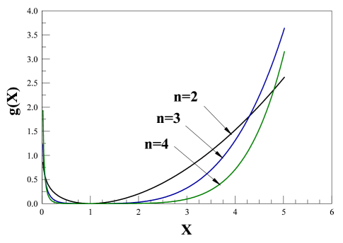
which leads to a strongly coupled regime. The results of a numerical analysis are depicted in fig. 2.
Refer to caption
Figure 2: The coupling g𝑔g as a function of X𝑋X, for the degrees of the new inflation potential n=2, 3, 4𝑛234n=2,\;3,\;4. For X1,g𝑋1𝑔X\to 1,\;g vanishes as [1X2]2(n1)superscriptdelimited-[]1𝑋22𝑛1\left[\frac{1-X}{2}\right]^{2\,(n-1)}. The point X=1,g=0formulae-sequence𝑋1𝑔0X=1,\;g=0 corresponds to the monomial m2ϕ2/2superscript𝑚2superscriptitalic-ϕ22m^{2}\;\phi^{2}/2. g𝑔g increases both for X0𝑋0X\to 0 and for large X𝑋X as, (log1X)n1superscript1𝑋𝑛1\left(\log\frac{1}{X}\right)^{n-1} and (X24n)n1superscriptsuperscript𝑋24𝑛𝑛1\left(\frac{X^{2}}{4\,n}\right)^{n-1}, respectively.

Before we proceed with a numerical study of the CMB indices and the tensor to scalar ratio, we can extract interesting and relevant information by focusing on the region X1similar-to𝑋1X\sim 1 which as discussed above corresponds to a weakly coupled family for broken symmetry potentials. This is the region near the minimum of the potential and the integral In(X)subscript𝐼𝑛𝑋I_{n}(X) can be evaluated simply by expanding w(χ)𝑤𝜒w(\chi) and its derivative near the minimum. To leading order in (X1)𝑋1(X-1) the condition (46) leads to eq.(49) and

(χcχ0)2=4or|χcχ0|=2.formulae-sequencesuperscriptsubscript𝜒𝑐subscript𝜒024orsubscript𝜒𝑐subscript𝜒02(\chi_{c}-\chi_{0})^{2}=4\quad{\rm or}\quad|\chi_{c}-\chi_{0}|=2\;. (51)

This is precisely eq.(26) for n=1𝑛1n=1 upon the shift χcχcχ0subscript𝜒𝑐subscript𝜒𝑐subscript𝜒0\chi_{c}\to\chi_{c}-\chi_{0}. Namely, eq.(51) is the condition eq.(26) for the quadratic monomial potential with minimum at χ=χ0𝜒subscript𝜒0\chi=\chi_{0} instead of χ=0𝜒0\chi=0 as in eq.(25). This is clearly a consequence of the fact that near the minimum X=1𝑋1X=1 the potential is quadratic, therefore for X1similar-to𝑋1X\sim 1 the quadratic monomial is an excellent approximation to the family of higher degree potentials and more so because g0similar-to𝑔0g\sim 0. For X1similar-to𝑋1X\sim 1 we find to leading order in (X1)𝑋1(X-1) the values:

ϵv=ηv=0.01(50Ne),ns=0.96+0.04(Ne50Ne),r=0.16(50Ne),dnsdlnk=0.0008(50Ne)2.\epsilon_{v}=\eta_{v}=0.01~{}\Big{(}\frac{50}{N_{e}}\Big{)}\quad,\quad n_{s}=0.96+0.04~{}\Big{(}\frac{N_{e}-50}{N_{e}}\Big{)}\quad,\quad r=0.16~{}\Big{(}\frac{50}{N_{e}}\Big{)}\quad,\quad\frac{dn_{s}}{d\ln k}=-0.0008~{}\Big{(}\frac{50}{N_{e}}\Big{)}^{2}\;. (52)

The fact that the potential eq.(43) is quadratic around the minimum X=1𝑋1X=1 explains why we have in this limit identical results for new inflation with the potential eq.(43) and chaotic inflation with the monomial potential m2ϕ2/2superscript𝑚2superscriptitalic-ϕ22m^{2}\;\phi^{2}/2.

As observed in WMAP3 these values of r,ns𝑟subscript𝑛𝑠r,\;n_{s} for Ne50similar-tosubscript𝑁𝑒50N_{e}\sim 50 yield a good fit to the available CMB data.

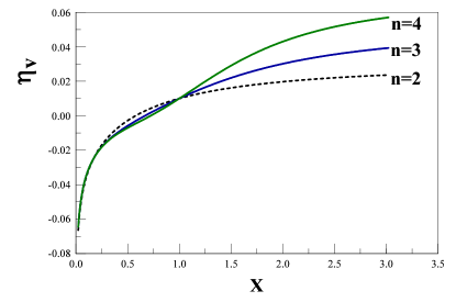
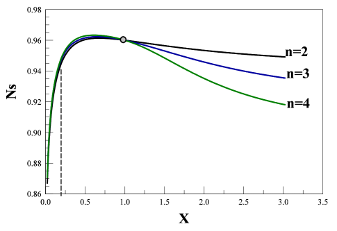
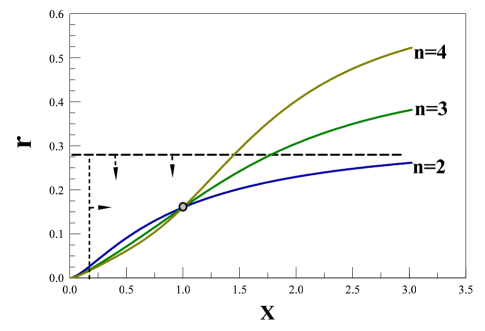
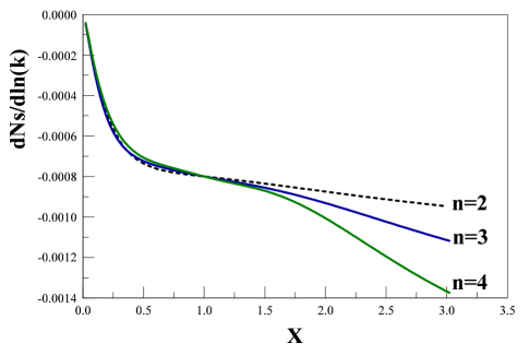
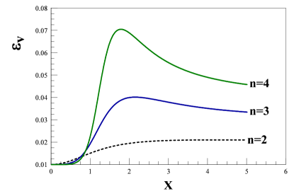
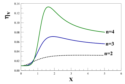
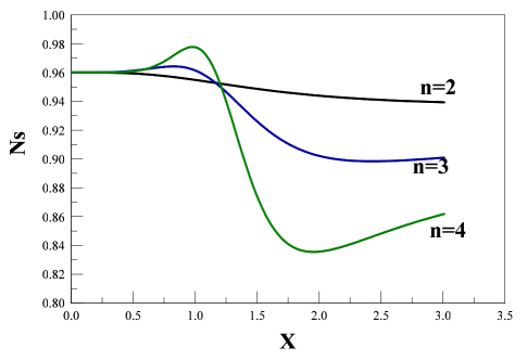
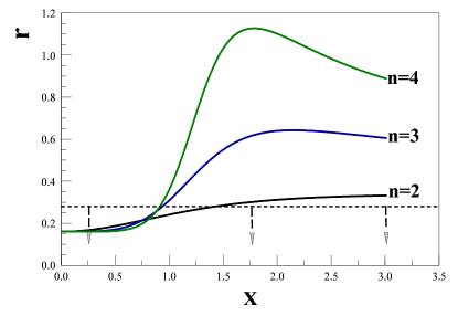
The results of the numerical analysis for ϵv,ηv,ns,rsubscriptitalic-ϵ𝑣subscript𝜂𝑣subscript𝑛𝑠𝑟\epsilon_{v},\;\eta_{v},\;n_{s},\;r and dns/dlnk𝑑subscript𝑛𝑠𝑑𝑘dn_{s}/d\ln k for the baseline value Ne=50subscript𝑁𝑒50N_{e}=50 are depicted in fig. 3, 4, 5 and 6 respectively.
Refer to caption
Refer to caption
Figure 3: Slow roll parameters as a function of X𝑋X for Ne=50subscript𝑁𝑒50N_{e}=50. Left panel ϵvsubscriptitalic-ϵ𝑣\epsilon_{v}, right panel ηvsubscript𝜂𝑣\eta_{v}, for new inflation with the degrees of the potential n=2,3,4𝑛234n=2,3,4. The results for arbitrary values of Nesubscript𝑁𝑒N_{e} are obtained by multiplying by the factor 50Ne50subscript𝑁𝑒\frac{50}{N_{e}}.
Refer to caption
Figure 4: Scalar spectral index nssubscript𝑛𝑠n_{s} for the degrees of the potential n=2,3,4𝑛234n=2,3,4 for new inflation with Ne=50subscript𝑁𝑒50N_{e}=50. The vertical line delimits the smallest value of nssubscript𝑛𝑠n_{s} (for r=0𝑟0r=0) WMAP3 . The grey dot at ns=0.96,X=1formulae-sequencesubscript𝑛𝑠0.96𝑋1n_{s}=0.96,\;X=1 corresponds to the value for the monomial potential n=1,m2ϕ2/2𝑛1superscript𝑚2superscriptitalic-ϕ22n=1,\;m^{2}\;\phi^{2}/2. Notice that the small field behavior is n𝑛n independent. For arbitrary Nesubscript𝑁𝑒N_{e} the result follows directly from the Ne=50subscript𝑁𝑒50N_{e}=50 value by using eq.(19).
Refer to caption
Figure 5: Tensor to scalar ratio r𝑟r vs. X𝑋X for the degrees of the potential n=2, 3, 4𝑛234n=2,\;3,\;4 for new inflation with Ne=50subscript𝑁𝑒50N_{e}=50. The horizontal dashed line corresponds to the upper limit r=0.28(95%CL)𝑟0.28percent95𝐶𝐿r=0.28~{}(95\%CL) from WMAP3 without running. The vertical dashed line determines the minimum value of X,X0.2similar-to𝑋𝑋0.2X,\;X\sim 0.2, consistent with the WMAP limits for nssubscript𝑛𝑠n_{s} as in fig. 4. The grey dot at X=1,r=0.16formulae-sequence𝑋1𝑟0.16X=1,\;r=0.16 corresponds to the value for the monomial potential m2ϕ2/2superscript𝑚2superscriptitalic-ϕ22m^{2}\;\phi^{2}/2. The small field limit is nearly independent of n𝑛n. For arbitrary Nesubscript𝑁𝑒N_{e} the result follows directly from the Ne=50subscript𝑁𝑒50N_{e}=50 value by using eq. (19).
Refer to caption
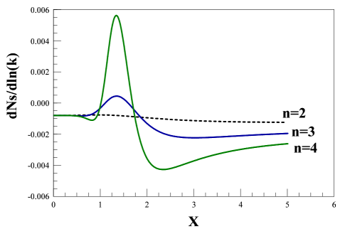
Figure 6: Running of the scalar index dns/dlnk𝑑subscript𝑛𝑠𝑑𝑘dn_{s}/d\ln k vs. X𝑋X for the degrees of the potential n=2,3,4𝑛234n=2,3,4 respectively for new inflation with Ne=50subscript𝑁𝑒50N_{e}=50. The small field behavior is independent of n𝑛n. For arbitrary Nesubscript𝑁𝑒N_{e} the result follows directly from the Ne=50subscript𝑁𝑒50N_{e}=50 value by using eq. (19).

The vertical dashed line in fig. 4 at X0.2similar-to𝑋0.2X\sim 0.2 determines the lower limit of X𝑋X for which nssubscript𝑛𝑠n_{s} is consistent with the WMAP data for r=0𝑟0r=0. For large values of X,ns𝑋subscript𝑛𝑠X,\;n_{s} approaches asymptotically the values for the monomial potentials ϕ2nsuperscriptitalic-ϕ2𝑛\phi^{2\,n} given by eq. (29). For the larger degrees n𝑛n, the asymptotic behavior of nssubscript𝑛𝑠n_{s} and r𝑟r settles at larger values of X𝑋X, this is a consequence of the larger region in which the coupling is small as observed in fig. 2 for larger degrees n𝑛n. The horizontal dashed lines with vertical downward arrows in fig. 5 determines the upper bound from WMAP WMAP3 given by eq. (22) without running, since from fig. 6 the values of dns/dlnk𝑑subscript𝑛𝑠𝑑𝑘dn_{s}/d\ln k for these models are negligible. The vertical dashed line with the right-pointing arrow in fig. 5 determines the values of X𝑋X for which nssubscript𝑛𝑠n_{s} are consistent with the WMAP data (see also fig. 4).

From these figures we see that unlike the case of a pure monomial potential λϕ2n𝜆superscriptitalic-ϕ2𝑛\lambda\,\phi^{2\,n} with n2𝑛2n\geq 2, there is a large region of field space within which the new inflation models given by eq.(30) are consistent with the bounds from marginalized WMAP3 data and the combined WMAP3 + LSS data WMAP3 .

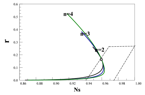
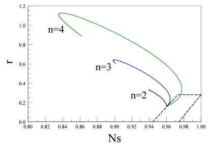
Fig. 7 displays r𝑟r vs nssubscript𝑛𝑠n_{s} for the values n=2,3,4𝑛234n=2,3,4 in new inflation and indicate the trend with n𝑛n. While r𝑟r is a monotonically increasing function of X,ns𝑋subscript𝑛𝑠X,\;n_{s} features a maximum as a function of X𝑋X, hence r𝑟r becomes a double-valued function of nssubscript𝑛𝑠n_{s}. The grey dot at r=0.16,ns=0.96formulae-sequence𝑟0.16subscript𝑛𝑠0.96r=0.16,\;n_{s}=0.96 corresponds to the monomial potential m2ϕ2/2superscript𝑚2superscriptitalic-ϕ22m^{2}\;\phi^{2}/2 for Ne=50subscript𝑁𝑒50N_{e}=50. Values below the grey dot along the curve in fig. 7 correspond to small fields X<1𝑋1X<1 while values above it correspond to large fields X>1𝑋1X>1. We see from figs. 5 and 7 that large fields systematically lead to larger values of r𝑟r. Models that fit the WMAP data to 95%CLpercent95𝐶𝐿95\%~{}CL are within the tilted box in fig. 7. The tilt accounts for the growth of the preferred value of nssubscript𝑛𝑠n_{s} with r𝑟r WMAP3 according to eq. (23).

Refer to caption
Figure 7: Tensor to scalar ratio r𝑟r vs. nssubscript𝑛𝑠n_{s} for degrees of the potential n=2, 3, 4𝑛234n=2,\,3,\,4 respectively for new inflation with Ne=50subscript𝑁𝑒50N_{e}=50. r𝑟r turns to be a double-valued function of nssubscript𝑛𝑠n_{s} exhibiting a maximum value for nssubscript𝑛𝑠n_{s}. The values inside the box between the dashed lines correspond to the WMAP3 marginalized region of the (ns,r)subscript𝑛𝑠𝑟(n_{s},r) plane with (95%CL):r<0.28, 0.942+0.12rns0.974+0.12r:percent95𝐶𝐿formulae-sequence𝑟0.280.9420.12𝑟subscript𝑛𝑠0.9740.12𝑟(95\%CL):\;r<0.28,\;0.942+0.12~{}r\leq n_{s}\leq 0.974+0.12~{}r, see eq.(23). The grey dot corresponds to the values for the monomial potential m2ϕ2/2superscript𝑚2superscriptitalic-ϕ22m^{2}\phi^{2}/2 and the value X=1:r=0.16,ns=0.96:𝑋1formulae-sequence𝑟0.16subscript𝑛𝑠0.96X=1:\;r=0.16,\;n_{s}=0.96.
Refer to caption
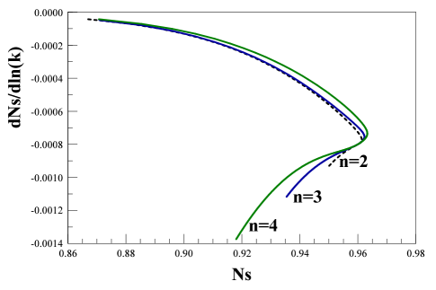
Figure 8: Running of the scalar index dns/dlnk𝑑subscript𝑛𝑠𝑑𝑘dn_{s}/d\ln k vs. nssubscript𝑛𝑠n_{s} for degrees of the potential n=2, 3, 4𝑛234n=2,\,3,\,4 respectively for new inflation with Ne=50subscript𝑁𝑒50N_{e}=50. The values for arbitrary Nesubscript𝑁𝑒N_{e} follow directly from the Ne=50subscript𝑁𝑒50N_{e}=50 value by using eq. (19).

Fig. 8 displays the running of the scalar index vs. nssubscript𝑛𝑠n_{s} for the different members of the family of new inflation showing clearly that running is all but negligible in the entire range of values consistent with the WMAP data. This was expected since the running in slow-roll is of the order 1Ne24×104similar-toabsent1superscriptsubscript𝑁𝑒2similar-to-or-equals4superscript104\sim\frac{1}{N_{e}^{2}}\simeq 4\times 10^{-4} [see eq.(18)] 1sN .

We note that dns/dlnk𝑑subscript𝑛𝑠𝑑𝑘dn_{s}/d\ln k is a monotonically decreasing function of X𝑋X approaching asymptotically the values for the monomials ϕ2nsuperscriptitalic-ϕ2𝑛\phi^{2\,n} given by eq. (29). X0.2similar-to𝑋0.2X\sim 0.2 which is the minimum value of X𝑋X consistent with the bounds from WMAP on nssubscript𝑛𝑠n_{s} (see fig. 4).

IV.1 Field reconstruction

The above analysis suggests to study the inverse problem, namely, for a given member of the family labeled by n𝑛n, we may ask what is the value ϕcsubscriptitalic-ϕ𝑐\phi_{c} of the field at Hubble crossing and what is the scale ϕ0subscriptitalic-ϕ0\phi_{0} of symmetry breaking of the potential which are consistent with the CMB+LSS data. This is tantamount to the program of reconstruction of the inflaton potential advocated in ref. reco and is achieved as follows: eq.(46) yields χ0=χ0[X]subscript𝜒0subscript𝜒0delimited-[]𝑋\chi_{0}=\chi_{0}[X] from which we obtain χc=χ0Xsubscript𝜒𝑐subscript𝜒0𝑋\chi_{c}=\chi_{0}\;X. These results are then input into the expression for nssubscript𝑛𝑠n_{s} by evaluating the potential w(χ)𝑤𝜒w(\chi) and its derivatives at the value of χcsubscript𝜒𝑐\chi_{c}. This yields ns=ns[χc]subscript𝑛𝑠subscript𝑛𝑠delimited-[]subscript𝜒𝑐n_{s}=n_{s}[\chi_{c}] which is then inverted to obtain χc=χc[ns]subscript𝜒𝑐subscript𝜒𝑐delimited-[]subscript𝑛𝑠\chi_{c}=\chi_{c}[n_{s}] and thus ϕcsubscriptitalic-ϕ𝑐\phi_{c}.

In the region X1similar-to𝑋1X\sim 1 corresponding to the weakly coupled case, this reconstruction program can be carried out as a systematic series in

ΔX1=χcχ01,Δ𝑋1subscript𝜒𝑐subscript𝜒01\Delta\equiv X-1=\frac{\chi_{c}}{\chi_{0}}-1\;, (53)

by expanding the inflationary potential and its derivatives in a power series in x𝑥x around x=1𝑥1x=1 in the integrand of In(X)subscript𝐼𝑛𝑋I_{n}(X) [eq. (47)]. For X=1𝑋1X=1 the value of the scalar index nssubscript𝑛𝑠n_{s} is determined by the simple monomial m2ϕ2/2superscript𝑚2superscriptitalic-ϕ22m^{2}\;\phi^{2}/2 which from eq. (28) for n=1𝑛1n=1 is given by ns1=2/Nesubscript𝑛𝑠12subscript𝑁𝑒n_{s}-1=-2/N_{e}. Therefore, in terms of nssubscript𝑛𝑠n_{s}, the actual expansion parameter is ns1+2/Nesubscript𝑛𝑠12subscript𝑁𝑒n_{s}-1+2/N_{e}.

We obtain nssubscript𝑛𝑠n_{s} to first order in ΔΔ\Delta from eqs.(10), (16), (43), (49) and (53) with the result,

ns1=2Ne[1+2n118Δ+𝒪(Δ2)]subscript𝑛𝑠12subscript𝑁𝑒delimited-[]12𝑛118Δ𝒪superscriptΔ2n_{s}-1=-\frac{2}{N_{e}}\left[1+\frac{2\,n-1}{18}\;\Delta+{\cal O}(\Delta^{2})\right]

then, by inverting this equation we find:

Δ(ns,n)=X1=9Ne2n1(ns1+2Ne)+𝒪([ns1+2Ne]2),Δsubscript𝑛𝑠𝑛𝑋19subscript𝑁𝑒2𝑛1subscript𝑛𝑠12subscript𝑁𝑒𝒪superscriptdelimited-[]subscript𝑛𝑠12subscript𝑁𝑒2\Delta(n_{s},n)=X-1=-\frac{9N_{e}}{2\,n-1}\left(n_{s}-1+\frac{2}{N_{e}}\right)+\mathcal{O}\left(\left[n_{s}-1+\frac{2}{N_{e}}\right]^{2}\right)\;, (54)

and from eqs. (49) and (54) we find,

χ0(ns,n)=2(2n1)9Ne|ns1+2Ne|[1Ne2(ns1+2Ne)]+𝒪([ns1+2Ne])subscript𝜒0subscript𝑛𝑠𝑛22𝑛19subscript𝑁𝑒subscript𝑛𝑠12subscript𝑁𝑒delimited-[]1subscript𝑁𝑒2subscript𝑛𝑠12subscript𝑁𝑒𝒪delimited-[]subscript𝑛𝑠12subscript𝑁𝑒\chi_{0}(n_{s},n)=\frac{2\;(2\,n-1)}{9\,N_{e}\left|n_{s}-1+\frac{2}{N_{e}}\right|}\left[1-\frac{N_{e}}{2}\left(n_{s}-1+\frac{2}{N_{e}}\right)\right]+\mathcal{O}\left(\left[n_{s}-1+\frac{2}{N_{e}}\right]\right) (55)

The leading order (1/Δproportional-toabsent1Δ\propto 1/\Delta) of this result for χ0(ns,n)subscript𝜒0subscript𝑛𝑠𝑛\chi_{0}(n_{s},n) can be simply cast as eq.(51): this is recognized as the condition to have 505050 e-folds for the quadratic monomial centered in the broken symmetry minimum [see discussion below eq. (51)].

Finally, the value of the (dimensionless) field χcsubscript𝜒𝑐\chi_{c} at Hubble crossing is determined from χc(ns,n)=χ0[1+Δ(ns,n)]subscript𝜒𝑐subscript𝑛𝑠𝑛subscript𝜒0delimited-[]1Δsubscript𝑛𝑠𝑛\chi_{c}(n_{s},n)=\chi_{0}\;[1+\Delta(n_{s},n)] from which we obtain

χc=2(2n1)9Ne|ns1+2Ne|[1(2n+17)Ne2(2n1)(ns1+2Ne)]+𝒪([ns1+2Ne]).subscript𝜒𝑐22𝑛19subscript𝑁𝑒subscript𝑛𝑠12subscript𝑁𝑒delimited-[]12𝑛17subscript𝑁𝑒22𝑛1subscript𝑛𝑠12subscript𝑁𝑒𝒪delimited-[]subscript𝑛𝑠12subscript𝑁𝑒\chi_{c}=\frac{2\;(2\,n-1)}{9\,N_{e}\left|n_{s}-1+\frac{2}{N_{e}}\right|}\left[1-\frac{(2\,n+17)\;N_{e}}{2\;(2\,n-1)}\left(n_{s}-1+\frac{2}{N_{e}}\right)\right]+\mathcal{O}\left(\left[n_{s}-1+\frac{2}{N_{e}}\right]\right)\;. (56)

The coupling constant g𝑔g can be also expressed in terms of nssubscript𝑛𝑠n_{s} in this regime with the result,

g=[9Ne|ns1+2Ne|2(2n1)]2n20,𝑔superscriptdelimited-[]9subscript𝑁𝑒subscript𝑛𝑠12subscript𝑁𝑒22𝑛12𝑛20g=\left[\frac{9\,N_{e}\left|n_{s}-1+\frac{2}{N_{e}}\right|}{2\;(2\,n-1)}\right]^{2\,n-2}\to 0\;,

which exhibits the weak coupling character of this limit.

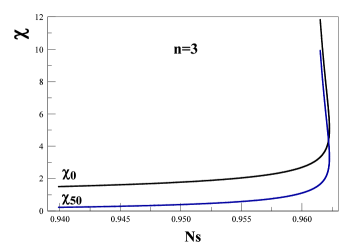
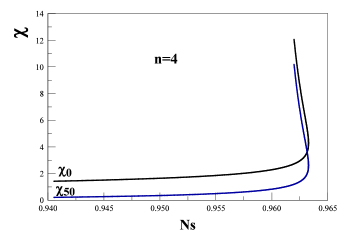
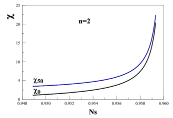
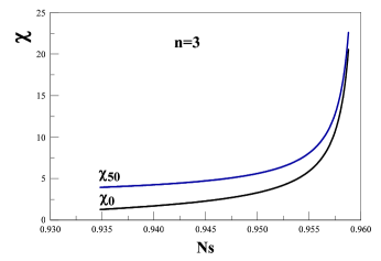
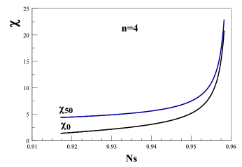
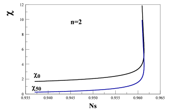
This analysis shows that the region in field space that corresponds to the region in nssubscript𝑛𝑠n_{s} that best fits the WMAP data can be systematically reconstructed in an expansion in ns1+2/Nesubscript𝑛𝑠12subscript𝑁𝑒n_{s}-1+2/N_{e}. This is yet another bonus of the 1/Ne1subscript𝑁𝑒1/N_{e} expansion. Although the above analysis can be carried out to an arbitrary order in ns1+2/Nesubscript𝑛𝑠12subscript𝑁𝑒n_{s}-1+2/N_{e}, it is more convenient to perform a numerical study of the region outside from X1similar-to𝑋1X\sim 1 to find the values of χcsubscript𝜒𝑐\chi_{c} and χ0subscript𝜒0\chi_{0} as a function of nssubscript𝑛𝑠n_{s} for fixed values of n,Ne𝑛subscript𝑁𝑒n,\;N_{e}. Figures 9 and 10 display χc,χ0subscript𝜒𝑐subscript𝜒0\chi_{c},\;\chi_{0} as a function of nssubscript𝑛𝑠n_{s} with Ne=50subscript𝑁𝑒50N_{e}=50 for different values of n𝑛n for the small field region X<1𝑋1X<1 and the large field region X>1𝑋1X>1 respectively. The point X=1𝑋1X=1 is a degeneracy point and corresponds to the quadratic monomial as discussed above.
Refer to caption
Refer to caption
Refer to caption
Figure 9: Reconstruction program for broken symmetry potentials with Ne=50subscript𝑁𝑒50N_{e}=50, small field case X<1.χ50χcformulae-sequence𝑋1subscript𝜒50subscript𝜒𝑐X<1.\;\chi_{50}\equiv\chi_{c} and χ0subscript𝜒0\chi_{0} vs. nssubscript𝑛𝑠n_{s} for degrees of the potential n=2,3,4𝑛234n=2,3,4, respectively. These values of χc,nssubscript𝜒𝑐subscript𝑛𝑠\chi_{c},\;n_{s} correspond to the region r<0.16𝑟0.16r<0.16.
Refer to caption
Refer to caption
Refer to caption
Figure 10: Reconstruction Program for broken symmetry potentials with Ne=50subscript𝑁𝑒50N_{e}=50, large field case X>1𝑋1X>1. χ50χcsubscript𝜒50subscript𝜒𝑐\chi_{50}\equiv\chi_{c} and χ0subscript𝜒0\chi_{0} vs. nssubscript𝑛𝑠n_{s} for degrees of the potential n=2,3,4𝑛234n=2,3,4, respectively. These values of χ,ns𝜒subscript𝑛𝑠\chi,\;n_{s} correspond to the region r>0.16𝑟0.16r>0.16.

Finally, the values for the dimensionful field ϕitalic-ϕ\phi are given by ϕc=NeMPlχc,ϕ0=NeMPlχ0formulae-sequencesubscriptitalic-ϕ𝑐subscript𝑁𝑒subscript𝑀𝑃𝑙subscript𝜒𝑐subscriptitalic-ϕ0subscript𝑁𝑒subscript𝑀𝑃𝑙subscript𝜒0\phi_{c}=\sqrt{N_{e}}\;M_{Pl}\;\chi_{c},\;\phi_{0}=\sqrt{N_{e}}\;M_{Pl}\;\chi_{0}. Figures 7, 9 and 10 lead to the conclusion that for the range of CMB parameters r<0.1𝑟0.1r<0.1 and ns0.96subscript𝑛𝑠0.96n_{s}\leq 0.96, the typical value of the symmetry breaking scale is ϕ010MPlsimilar-tosubscriptitalic-ϕ010subscript𝑀𝑃𝑙\phi_{0}\sim 10\;M_{Pl} and the value of the inflaton field at which cosmologically relevant wavelengths crossed the Hubble radius during new inflation is ϕcMPlsimilar-tosubscriptitalic-ϕ𝑐subscript𝑀𝑃𝑙\phi_{c}\sim M_{Pl} with a weak dependence on n𝑛n. For 0.1<r<0.160.1𝑟0.160.1<r<0.16 we have |ϕcϕ0|15MPlsimilar-tosubscriptitalic-ϕ𝑐subscriptitalic-ϕ015subscript𝑀𝑃𝑙|\phi_{c}-\phi_{0}|\sim 15\;M_{Pl}.

We obtain for the coupling g𝑔g in the X0𝑋0X\to 0 limit which is a strong coupling regime [see eq.(48)] where ns1much-less-thansubscript𝑛𝑠1n_{s}\ll 1,

g=[Ne4(11n)(1ns)]n1.𝑔superscriptdelimited-[]subscript𝑁𝑒411𝑛1subscript𝑛𝑠𝑛1g=\left[\frac{N_{e}}{4}\;\left(1-\frac{1}{n}\right)(1-n_{s})\right]^{n-1}\;.

Finally, we have the X𝑋X\to\infty limit which is also a strong coupling limit [see eq.(50)] where ns1(n+1)/Nesubscript𝑛𝑠1𝑛1subscript𝑁𝑒n_{s}\to 1-(n+1)/N_{e} and we find,

χ02=(4n)2[Ne(1ns)(n+1)4n(n1)+3(1+1n2)]1n10subscriptsuperscript𝜒20superscript4𝑛2superscriptdelimited-[]subscript𝑁𝑒1subscript𝑛𝑠𝑛14𝑛𝑛1311𝑛21𝑛10\displaystyle\chi^{2}_{0}=(4\,n)^{2}\left[\frac{N_{e}(1-n_{s})-(n+1)}{4\,n(n-1)+3\,\left(1+\frac{1}{n-2}\right)}\right]^{\frac{1}{n-1}}\to 0 (57)
(58)
g=4n(n1)+3(1+1n2)(4n)n1[Ne(1ns)(n+1)].𝑔4𝑛𝑛1311𝑛2superscript4𝑛𝑛1delimited-[]subscript𝑁𝑒1subscript𝑛𝑠𝑛1\displaystyle g=\frac{4\,n(n-1)+3\,\left(1+\frac{1}{n-2}\right)}{(4\,n)^{n-1}\;\left[N_{e}(1-n_{s})-(n+1)\right]}\to\infty\;. (59)

V Chaotic inflation models.

We now turn to the study of the family of chaotic inflationary potentials given by eq. (44). Taking that the end of inflation corresponds to x=0𝑥0x=0, the condition eq.(9) now becomes

2nχ02=Jn(X)=0Xn+x2n21+x2n2x𝑑x.2𝑛subscriptsuperscript𝜒20subscript𝐽𝑛𝑋subscriptsuperscript𝑋0𝑛superscript𝑥2𝑛21superscript𝑥2𝑛2𝑥differential-d𝑥\frac{2\,n}{\chi^{2}_{0}}=J_{n}(X)=\int^{X}_{0}\frac{n+x^{2\,n-2}}{1+x^{2\,n-2}}~{}x~{}{dx}\,. (60)

Again, this integral can be computed in closed form in terms of hypergeometric functions gr which can be reduced to a finite sum of elementary functionspru . For general values of X𝑋X the integral will be studied numerically, but the small X𝑋X region can be studied by expanding the integrand in powers of x2n2superscript𝑥2𝑛2x^{2\,n-2}, with the result

1=χ02X24[1n1n2X2n2+𝒪(X4n4)].1subscriptsuperscript𝜒20superscript𝑋24delimited-[]1𝑛1superscript𝑛2superscript𝑋2𝑛2𝒪superscript𝑋4𝑛41=\frac{\chi^{2}_{0}\,X^{2}}{4}\left[1-\frac{n-1}{n^{2}}\;X^{2\,n-2}+\mathcal{O}(X^{4\,n-4})\right]\;. (61)

For small X𝑋X and recalling that X=χc/χ0𝑋subscript𝜒𝑐subscript𝜒0X=\chi_{c}/\chi_{0} this relation yields

|χc|=2[1+n12n2X2n2+𝒪(X4n4)]subscript𝜒𝑐2delimited-[]1𝑛12superscript𝑛2superscript𝑋2𝑛2𝒪superscript𝑋4𝑛4|\chi_{c}|=2\left[1+\frac{n-1}{2\,n^{2}}\;X^{2\,n-2}+\mathcal{O}(X^{4\,n-4})\right] (62)

which is again, at dominant order the relation for the quadratic monomial potential eq.(26) for n=1𝑛1n=1. This must be the case because the small field limit is dominated by the quadratic term in the potential. For small fields, χ02/Xsubscript𝜒02𝑋\chi_{0}\approx 2/X and the coupling g𝑔g vanishes as,

g(X)=X0(X2)2n2.superscript𝑋0𝑔𝑋superscript𝑋22𝑛2g(X)\buildrel X\to 0\over{=}\left(\frac{X}{2}\right)^{2\,n-2}\;. (63)

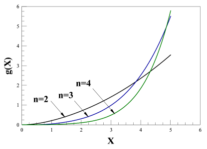
The coupling as a function of X𝑋X is shown in fig. 11.

Refer to caption
Figure 11: Coupling g𝑔g as a function of X𝑋X for Ne=50subscript𝑁𝑒50N_{e}=50, for n=2,3,4𝑛234n=2,3,4 for chaotic inflation. g𝑔g turns to be a monotonically increasing function of X𝑋X. g𝑔g vanishes for X0𝑋0X\to 0 as (X2)2n2superscript𝑋22𝑛2\left(\frac{X}{2}\right)^{2\,n-2} in sharp contrast with new inflation where g𝑔g strongly increases for X0𝑋0X\to 0.

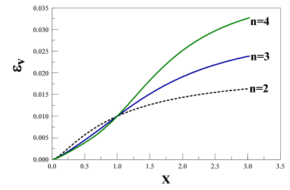
The dependence of ϵv,ηvsubscriptitalic-ϵ𝑣subscript𝜂𝑣\epsilon_{v},\;\eta_{v} in the full range of X𝑋X for several representative values of n𝑛n is studied numerically: these results are displayed in fig. 12. In the small X𝑋X regime, we obtain from eqs. (10), (44) and (61) the expressions,

ϵv=12Ne[1+(2n1)(n1)n2X2n2+𝒪(X4n4)]subscriptitalic-ϵ𝑣12subscript𝑁𝑒delimited-[]12𝑛1𝑛1superscript𝑛2superscript𝑋2𝑛2𝒪superscript𝑋4𝑛4\displaystyle\epsilon_{v}=\frac{1}{2\,N_{e}}\left[1+\frac{(2\,n-1)(n-1)}{n^{2}}\;X^{2\,n-2}+\mathcal{O}\left(X^{4\,n-4}\right)\right] (64)
ηv=12Ne[1+(2n1)(n21)n2X2n2+𝒪(X4n4)]subscript𝜂𝑣12subscript𝑁𝑒delimited-[]12𝑛1superscript𝑛21superscript𝑛2superscript𝑋2𝑛2𝒪superscript𝑋4𝑛4\displaystyle\eta_{v}=\frac{1}{2\,N_{e}}\left[1+\frac{(2\,n-1)(n^{2}-1)}{n^{2}}X^{2\,n-2}+\mathcal{O}\left(X^{4\,n-4}\right)\right] (65)

As X0,ϵv𝑋0subscriptitalic-ϵ𝑣X\rightarrow 0,\;\epsilon_{v} and ηvsubscript𝜂𝑣\eta_{v} tend to the result from the quadratic monomial potential, namely ϵv=ηv=1/[2Ne]subscriptitalic-ϵ𝑣subscript𝜂𝑣1delimited-[]2subscript𝑁𝑒\epsilon_{v}=\eta_{v}=1/[2\,N_{e}] as must be the case because the quadratic term dominates the potential for X1much-less-than𝑋1X\ll 1.

Figures 13, 14 display ns,rsubscript𝑛𝑠𝑟n_{s},\;r as functions of X𝑋X for Ne=50subscript𝑁𝑒50N_{e}=50 respectively. For X0,ns0.96formulae-sequence𝑋0subscript𝑛𝑠0.96X\rightarrow 0,\;n_{s}\rightarrow 0.96 and r0.16𝑟0.16r\rightarrow 0.16 which are the values from the quadratic monomial m2ϕ2/2superscript𝑚2superscriptitalic-ϕ22m^{2}\;\phi^{2}/2.

For X1much-greater-than𝑋1X\gg 1, the values of ns,rsubscript𝑛𝑠𝑟n_{s},\;r for the monomial potentials ϕ2nsuperscriptitalic-ϕ2𝑛\phi^{2\,n} are attained asymptotically, namely, (for Ne=50subscript𝑁𝑒50N_{e}=50): ns1=2(n+1)×102,r=0.16nformulae-sequencesubscript𝑛𝑠12𝑛1superscript102𝑟0.16𝑛n_{s}-1=-2\,(n+1)\times 10^{-2},\;r=0.16\,n.

Comparing figs. 13, 14 to those for the new inflation case, (figs. 4 and 5), we note that the range in which the chaotic family provide a good fit to the WMAP data is very much smaller than for new inflation. Fig. 13 shows that in chaotic inflation only for n=2𝑛2n=2 the range of nssubscript𝑛𝑠n_{s} is allowed by the WMAP data in a fairly extensive range of values of X𝑋X, whereas for n=3, 4𝑛34n=3,\;4 (and certainly larger), there is a relatively small window in field space for X<1𝑋1X<1 which satisfies the data for nssubscript𝑛𝑠n_{s} and r𝑟r simultaneously.

The tensor to scalar ratio r𝑟r in chaotic inflationary models is larger than 0.160.160.16 for all values of X𝑋X, approaching asymptotically for large X𝑋X the value r=0.16n𝑟0.16𝑛r=0.16\,n associated to the monomial potentials ϕ2nsuperscriptitalic-ϕ2𝑛\phi^{2\,n}.

Refer to caption
Refer to caption
Figure 12: Left panel ϵvsubscriptitalic-ϵ𝑣\epsilon_{v}, right pannel ηvsubscript𝜂𝑣\eta_{v} as a function of X𝑋X for Ne=50subscript𝑁𝑒50N_{e}=50, for chaotic inflation with degrees of the potential n=2,3,4𝑛234n=2,3,4. The small X𝑋X behavior is n𝑛n independent.
Refer to caption
Figure 13: Scalar spectral index nssubscript𝑛𝑠n_{s} for degrees of the potential n=2,3,4𝑛234n=2,3,4 respectively for chaotic inflation with Ne=50subscript𝑁𝑒50N_{e}=50. For X0,ns𝑋0subscript𝑛𝑠X\to 0,\;n_{s} reaches for all n𝑛n the value ns=0.96subscript𝑛𝑠0.96n_{s}=0.96 corresponding to the monomial potential m2ϕ2/2superscript𝑚2superscriptitalic-ϕ22m^{2}\phi^{2}/2.
Refer to caption
Figure 14: Tensor to scalar ratio r𝑟r vs. X𝑋X for degrees of the potential n=2,3,4𝑛234n=2,3,4 respectively for chaotic inflation with Ne=50subscript𝑁𝑒50N_{e}=50. The horizontal dashed lines with the downward arrows delimit the region of 95%CLpercent95𝐶𝐿95\%~{}CL given by WMAP3 with no running r<0.28𝑟0.28r<0.28 WMAP3 .

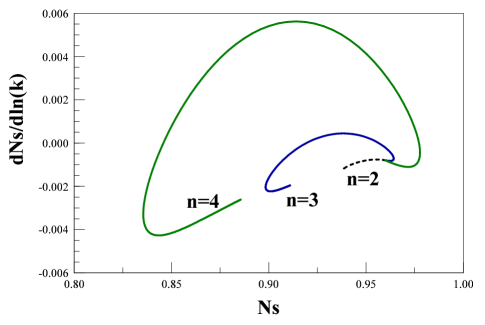
Fig. 15 displays dns/dlnk𝑑subscript𝑛𝑠𝑑𝑘dn_{s}/d\ln k as a function of X𝑋X, while the running is again negligible, it is strikingly different from the new inflation case. Again this figure, in combination with those for nssubscript𝑛𝑠n_{s} and r𝑟r as functions of X𝑋X distinctly shows that only n=2𝑛2n=2 in chaotic inflation is compatible with the bounds from the WMAP data, while for n=3,4𝑛34n=3,4 only a small window for X<1𝑋1X<1 is allowed by the data. We see from fig. 15 that dns/dlnk𝑑subscript𝑛𝑠𝑑𝑘dn_{s}/d\ln k takes negative as well as positive values for chaotic inflation, in contrast with new inflation where dns/dlnk<0𝑑subscript𝑛𝑠𝑑𝑘0dn_{s}/d\ln k<0.

Refer to caption
Figure 15: Running of the scalar index dns/dlnk𝑑subscript𝑛𝑠𝑑𝑘dn_{s}/d\ln k vs. X𝑋X for degrees of the potential n=2, 3, 4𝑛234n=2,\;3,\;4 respectively for chaotic inflation with Ne=50subscript𝑁𝑒50N_{e}=50. The X0𝑋0X\to 0 behavior is n𝑛n independent. dns/dlnk𝑑subscript𝑛𝑠𝑑𝑘dn_{s}/d\ln k features a maximun value that gets stronger with increasing n𝑛n. For chaotic inflation dns/dlnk𝑑subscript𝑛𝑠𝑑𝑘dn_{s}/d\ln k takes negative as well as positive values, in contrast with new inflation where dns/dlnk<0𝑑subscript𝑛𝑠𝑑𝑘0dn_{s}/d\ln k<0.

The fact that the combined bounds on ns,rsubscript𝑛𝑠𝑟n_{s},\;r and dns/dlnk𝑑subscript𝑛𝑠𝑑𝑘dn_{s}/d\ln k from the WMAP3 data WMAP3 provide much more stringent constraints on chaotic models is best captured by displaying r𝑟r as a function of nssubscript𝑛𝑠n_{s} in fig. 16. The region allowed by the WMAP data lies within the tilted box delimited by the vertical and horizontal dashed lines that represent the 95%CLpercent95𝐶𝐿95\%CL band WMAP3 .

Refer to caption
Figure 16: Tensor to scalar ratio r𝑟r vs. nssubscript𝑛𝑠n_{s} for degrees of the potential n=2, 3, 4𝑛234n=2,\;3,\;4 respectively for chaotic inflation with Ne=50subscript𝑁𝑒50N_{e}=50. The range of 95%CLpercent95𝐶𝐿95\%~{}CL as determined by WMAP3 WMAP3 is within the tilted box delimited by : r<0.28, 0.942+0.12rns0.974+0.12rformulae-sequence𝑟0.280.9420.12𝑟subscript𝑛𝑠0.9740.12𝑟r<0.28,\;0.942+0.12\,r\leq n_{s}\leq 0.974+0.12\,r, see eq.(23).

A complementary assessment of the allowed region for this family of effective field theories is shown in fig. 17 which distinctly shows that only the n=2𝑛2n=2 case of chaotic inflation is allowed by the WMAP3 data.
Refer to caption
Figure 17: Running of the scalar index dns/dlnk𝑑subscript𝑛𝑠𝑑𝑘dn_{s}/d\ln k vs. nssubscript𝑛𝑠n_{s} for degrees of the potential n=2, 3, 4𝑛234n=2,\,3,\,4 respectively for chaotic inflation with Ne=50subscript𝑁𝑒50N_{e}=50.

V.1 Field reconstruction

The reconstruction program proceeds in the same manner as in the case of new inflation: the first step is to obtain χ0(X)subscript𝜒0𝑋\chi_{0}(X) from eq.(60). Then ϵvsubscriptitalic-ϵ𝑣\epsilon_{v} and ηvsubscript𝜂𝑣\eta_{v} are obtained as a function of X𝑋X which yields ns(X)subscript𝑛𝑠𝑋n_{s}(X). Inverting this relation we find X=X(ns)𝑋𝑋subscript𝑛𝑠X=X(n_{s}) and finally χc(ns)=χ0X(ns)subscript𝜒𝑐subscript𝑛𝑠subscript𝜒0𝑋subscript𝑛𝑠\chi_{c}(n_{s})=\chi_{0}\;X(n_{s}). While this program must be carried out numerically, we can gain important insight by focusing on the small X𝑋X region and using eq.(61).

From eqs. (16), (64) and (65) we find

ns1+2Ne=X2n2(2n1)(n1)(n2)n2Ne+𝒪(X4n4)subscript𝑛𝑠12subscript𝑁𝑒superscript𝑋2𝑛22𝑛1𝑛1𝑛2superscript𝑛2subscript𝑁𝑒𝒪superscript𝑋4𝑛4n_{s}-1+\frac{2}{N_{e}}=X^{2\,n-2}\;\frac{(2\,n-1)(n-1)(n-2)}{n^{2}\,N_{e}}+\mathcal{O}\Big{(}X^{4n-4}\Big{)} (66)

As X0𝑋0X\rightarrow 0 it follows that ns12/Nesubscript𝑛𝑠12subscript𝑁𝑒n_{s}\rightarrow 1-2/N_{e} which is the value for the scalar index for the quadratic monomial potential m2ϕ2/2superscript𝑚2superscriptitalic-ϕ22m^{2}\phi^{2}/2. However, for n>2𝑛2n>2 this limit is approached from above, namely for n>2𝑛2n>2 it follows that ns>12/Nesubscript𝑛𝑠12subscript𝑁𝑒n_{s}>1-2/N_{e}. The small X𝑋X region corresponds to small departures of nssubscript𝑛𝑠n_{s} from the value determined by the quadratic monomial 12/Ne12subscript𝑁𝑒1-2/N_{e} but always larger than this value for n>2𝑛2n>2. In the small field limit we reconstruct the value of χcsubscript𝜒𝑐\chi_{c} in an expansion in ns1+2/Nesubscript𝑛𝑠12subscript𝑁𝑒n_{s}-1+2/N_{e}. The leading order in this expansion is obtained by combining eqs. (62) and (66), we obtain

|χc|=2[1+(ns1+2Ne)Ne2(2n1)(n2)]+𝒪([ns1+2/Ne]2)subscript𝜒𝑐2delimited-[]1subscript𝑛𝑠12subscript𝑁𝑒subscript𝑁𝑒22𝑛1𝑛2𝒪superscriptdelimited-[]subscript𝑛𝑠12subscript𝑁𝑒2|\chi_{c}|=2\Bigg{[}1+\frac{\big{(}n_{s}-1+\frac{2}{N_{e}}\big{)}N_{e}}{2\,(2\,n-1)\,(n-2)}\Bigg{]}+{\cal O}\left(\left[n_{s}-1+2/N_{e}\right]^{2}\right) (67)

Obviously, this leading order term is singular at n=2𝑛2n=2, this is a consequence of the result eq.(66) which entails that for n=2𝑛2n=2 the expansion must be pursued to higher order, up to X4n4superscript𝑋4𝑛4X^{4n-4}.

We find from eqs. (16), (64) and (65) for n=2𝑛2n=2,

ns1+2Ne=1724NeX4+𝒪(X6),n=2,n_{s}-1+\frac{2}{N_{e}}=-\frac{17}{24\,N_{e}}\;X^{4}+\mathcal{O}\Big{(}X^{6}\Big{)}\quad,\quad n=2\;, (68)

therefore,

|χc|=2[1+3Ne136(12Nens)]+𝒪(ns1+2Ne),n=2.|\chi_{c}|=2\Bigg{[}1+\sqrt{\frac{3\,N_{e}}{136}\left(1-\frac{2}{N_{e}}-n_{s}\right)}\,\Bigg{]}+{\cal O}\left(n_{s}-1+\frac{2}{N_{e}}\right)\quad,\quad n=2\;. (69)

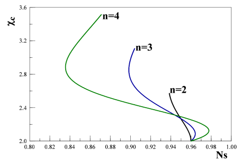
We see that the derivative of χcsubscript𝜒𝑐\chi_{c} with respect to nssubscript𝑛𝑠n_{s} is singular for n=2𝑛2n=2 at ns=12Nesubscript𝑛𝑠12subscript𝑁𝑒n_{s}=1-\frac{2}{N_{e}}. We note that for n=2𝑛2n=2 there is a sign change with respect to the cases n>2𝑛2n>2 and ns1+2/Ne0subscript𝑛𝑠12subscript𝑁𝑒0n_{s}-1+2/N_{e}\leq 0 as determined by eq. (68).

Fig. 18 shows χcsubscript𝜒𝑐\chi_{c} as a function of nssubscript𝑛𝑠n_{s} for n=2, 3, 4𝑛234n=2,\;3,\;4 for Ne=50subscript𝑁𝑒50N_{e}=50. The case n=2𝑛2n=2 clearly shows the singularity in the derivative χc/nssubscript𝜒𝑐subscript𝑛𝑠\partial\chi_{c}/\partial n_{s} at ns=12/Ne=0.96subscript𝑛𝑠12subscript𝑁𝑒0.96n_{s}=1-2/N_{e}=0.96 [see eq.(69)].

Combining fig. 18 with fig. 16 it is clear that there is a small window in field space within which chaotic models provide a good fit to the WMAP3 data, for Ne=50subscript𝑁𝑒50N_{e}=50 we find:

n=2:0.95ns0.960,2.0|χc|2.25\displaystyle n=2~{}:~{}~{}0.95\lesssim n_{s}\leq 0.960~{},~{}2.0\leq|\chi_{c}|\lesssim 2.25
n=3:0.96ns0.965,2.0|χc|2.15\displaystyle n=3~{}:~{}~{}0.96\leq n_{s}\lesssim 0.965~{},~{}2.0\leq|\chi_{c}|\lesssim 2.15
n=4:0.96ns0.975,2.0|χc|2.10.\displaystyle n=4~{}:~{}~{}0.96\leq n_{s}\leq 0.975~{},~{}2.0\leq|\chi_{c}|\lesssim 2.10\;. (70)

Restoring the dimensions via eq. (7) these values translate into a narrow region of width Δϕ1.5MPlless-than-or-similar-toΔitalic-ϕ1.5subscript𝑀𝑃𝑙\Delta\phi\lesssim 1.5\,M_{Pl} around the scale |ϕc|15MPlsimilar-tosubscriptitalic-ϕ𝑐15subscript𝑀𝑃𝑙|\phi_{c}|\sim 15~{}M_{Pl}.

Therefore, the joint analysis for ns,r,dns/dlnksubscript𝑛𝑠𝑟𝑑subscript𝑛𝑠𝑑𝑘n_{s},\;r,\;dn_{s}/d\ln k distinctly reveals that: (i) chaotic models favor larger values of r𝑟r thus, larger tensor amplitudes, and (ii) chaotic models feature smaller regions in field space consistent with the CMB and large scale structure data. Only the case n=2𝑛2n=2 features a larger region of consistency with the combined WMAP3 data.
Refer to caption
Figure 18: Reconstruction program for chaotic inflation with Ne=50subscript𝑁𝑒50N_{e}=50, χcsubscript𝜒𝑐\chi_{c} vs. nssubscript𝑛𝑠n_{s} for n=2, 3, 4𝑛234n=2,\,3,\,4 respectively.

VI Conclusions

The fact that current observations of the CMB and LSS are already placing constraints on inflationary models which will undoubtedly become more stringent with forthcoming observations, motivates a study of the predictions for the CMB power spectra from different inflationary scenarios. We perform a systematic study of families of single field new and chaotic inflation slow roll models characterized by effective field theories with potentials of the form

V(ϕ)𝑉italic-ϕ\displaystyle V(\phi) =\displaystyle= V012m2ϕ2+λ2nϕ2n,brokensymmetry\displaystyle V_{0}-\frac{1}{2}\;m^{2}\;\phi^{2}+\frac{\lambda}{2\,n}\;\phi^{2n}\quad,\quad{\rm broken~{}symmetry} (71)
V(ϕ)𝑉italic-ϕ\displaystyle V(\phi) =\displaystyle= 12m2ϕ2+λ2nϕ2n,unbrokensymmetry.\displaystyle\frac{1}{2}\;m^{2}\;\phi^{2}+\frac{\lambda}{2\,n}\;\phi^{2\,n}\quad,\quad{\rm unbroken~{}symmetry}\;. (72)

Unlike the approach followed in peiris ; WMAP3 based on the inflationary flow equationshoki , or more recent studies which focused on specific inflationary models salama , or on statistical analysis of models kinkol , we implement an expansion in 1/Ne1subscript𝑁𝑒1/N_{e} where Ne50similar-tosubscript𝑁𝑒50N_{e}\sim 50 is the number of e-folds before the end of inflation when wavelengths of cosmological relevance today cross the Hubble radius during inflation. We provide an analysis of the dependence of CMB observables (ns,rsubscript𝑛𝑠𝑟n_{s},\;r and dns/dlnk𝑑subscript𝑛𝑠𝑑𝑘dn_{s}/d\ln k) with n𝑛n and establish the region in field space within which these families provide a good agreement with the WMAP3 data combined with large scale surveys.

For new inflation models with potentials eq.(71) there are two distinct regions corresponding to values of the inflaton field smaller (small field) or larger (large field) than the symmetry breaking scale. For this family we find a wide range in the (ns,r)subscript𝑛𝑠𝑟(n_{s},r) plane in which the different members n=2, 3, 4𝑛234n=2,\;3,\;4... are allowed by the data both for small and large fields with negligible running of the scalar index:

4(n+1)×104dns/dlnk2×104.4𝑛1superscript104𝑑subscript𝑛𝑠𝑑𝑘2superscript104-4\;(n+1)\times 10^{-4}\leq dn_{s}/d\ln k\leq-2\times 10^{-4}\;.

For Ne=50subscript𝑁𝑒50N_{e}=50 the values ns=0.96,r=0.16formulae-sequencesubscript𝑛𝑠0.96𝑟0.16n_{s}=0.96,r=0.16 which are those determined by the simple monomial potential m2ϕ2/2superscript𝑚2superscriptitalic-ϕ22m^{2}\;\phi^{2}/2 determine a divide and a degeneracy point in the field and parameter space. Small field regions yield r<0.16𝑟0.16r<0.16 while large field regions correspond to r>0.16𝑟0.16r>0.16.

The 1/Ne1subscript𝑁𝑒1/N_{e} expansion also provides a powerful tool to implement a reconstruction program that allows to extract the value of the field Nesubscript𝑁𝑒N_{e} e-folds before the end of inflation, and in the case of new inflationary models, the symmetry breaking scale.

We find that the region of field space favored by the WMAP3 data can be explored in a systematic expansion in ns1+2/Nesubscript𝑛𝑠12subscript𝑁𝑒n_{s}-1+2/N_{e}. An analytic and numerical study of this region lead us to conclude that if forthcoming data on tensor modes favors r<0.16𝑟0.16r<0.16 then new inflation is favored, and we predict for r<0.1𝑟0.1r<0.1 that (i) the symmetry breaking scale is

ϕ010MPl,similar-tosubscriptitalic-ϕ010subscript𝑀𝑃𝑙\phi_{0}\sim 10~{}M_{Pl}\;,

and (ii) the value of the field when cosmologically relevant wavelengths cross the Hubble radius is |ϕc|MPlsimilar-tosubscriptitalic-ϕ𝑐subscript𝑀𝑃𝑙|\phi_{c}|\sim M_{Pl} .

The family of chaotic inflationary models characterized by the potentials eq.(72) feature tensor to scalar ratios r0.16𝑟0.16r\geq 0.16 (for Ne=50subscript𝑁𝑒50N_{e}=50), with the minimum, r=0.16𝑟0.16r=0.16 obtained in the limit of small inflaton amplitude and corresponds to the monomial potential m2ϕ2/2superscript𝑚2superscriptitalic-ϕ22m^{2}\;\phi^{2}/2 which is again a degeneracy point for this family of models.

The combined marginalized data from WMAP3 WMAP3 yields a very small window within which chaotic models are allowed by the data, the largest region of overlap with the (r,ns)𝑟subscript𝑛𝑠(r,n_{s}) WMAP3 data corresponds to n=2𝑛2n=2 and the width of the region decreases with larger n𝑛n. The typical scale of the field at Hubble crossing for these models is |ϕc|15MPlsimilar-tosubscriptitalic-ϕ𝑐15subscript𝑀𝑃𝑙|\phi_{c}|\sim 15~{}M_{Pl} (for Ne=50subscript𝑁𝑒50N_{e}=50). Some small regions in field space consistent with the WMAP3 data feature peaks in the running of the scalar index but in the region consistent with the WMAP3 data in chaotic inflation the running is again negligible. If future observations determine a tensor to scalar ratio r<0.16𝑟0.16r<0.16, such bound will, all by itself, rule out the large family of chaotic inflationary models of the form (72) for any n𝑛n.

Acknowledgements.
D. B. and C. M. Ho thank the US NSF for support under grant PHY-0242134, LPTHE and the Observatoire de Paris and LERMA for hospitality during this work. D.B. thanks A. Kosowsky for illuminating conversations.

References

  • (1) D. Kazanas, Astrophys. J 241, L59 (1980). A. Guth, Phys. Rev. D23, 347 (1981); astro-ph/0404546 (2004). K. Sato, Mon. Not. R. Astron. Soc. 195, 467 (1981).
  • (2) E. W. Kolb and M. S. Turner, The Early Universe Addison Wesley, Redwood City, C.A. 1990. P. Coles and F. Lucchin, Cosmology, John Wiley, Chichester, 1995. A. R. Liddle and D. H. Lyth, Cosmological Inflation and Large Scale Structure, Cambridge University Press, 2000. S. Dodelson, Modern Cosmology, Academic Press, 2003. D. H. Lyth , A. Riotto, Phys. Rept. 314, 1 (1999).
  • (3) V. F. Mukhanov , G. V. Chibisov, Soviet Phys. JETP Lett. 33, 532 (1981); V. F. Mukhanov, H. A. Feldman , R. H. Brandenberger, Phys. Rept. 215, 203 (1992). S. W. Hawking, Phys. Lett. B115, 295 (1982). A. H. Guth , S. Y. Pi, Phys. Rev. Lett. 49, 1110 (1982). A. A. Starobinsky, Phys. Lett. B117, 175 (1982). J. M. Bardeen, P. J. Steinhardt , M. S. Turner, Phys. Rev. D28, 679 (1983).
  • (4) C. L. Bennett et.al. (WMAP collaboration), Ap. J. Suppl. 148, 1 (2003). A. Kogut et.al. (WMAP collaboration), Ap. J. Suppl. 148, 161 (2003). D. N. Spergel et. al. (WMAP collaboration), Ap. J. Suppl. 148, 175 (2003).
  • (5) H. V. Peiris et.al. (WMAP collaboration), Ap. J. Suppl.148, 213 (2003).
  • (6) D. N. Spergel et. al. (WMAP collaboration), astro-ph/0603449.
  • (7) L. Page, et. al. (WMAP collaboration), astro-ph/0603450. G. Hinshaw,et. al. (WMAP collaboration), astro-ph/0603451. N. Jarosik, et. al. (WMAP collaboration), astro-ph/0603452.
  • (8) M. Tegmark et.al. Phys. Rev D69,103501, (2004) D. J. Eisenstein et.al. ApJ. 633, 560 (2005) U. Seljak et al., Phys. Rev. D71, 103515 (2005).
  • (9) A. G. Sánchez et. al., Mon. Not. Roy. Astron. Soc. 366, 189 (2006). S. Cole et.al. Mon. Not. Roy. Astron. Soc. 362, 505 (2005).
  • (10) A. G. Sanchez and C. M. Baugh, astro-ph/0612743.
  • (11) M. B. Hoffman and M. S. Turner, Phys. Rev. 64, 023506 (2001). W. H. Kinney, Phys. Rev. D66,083508 (2002).
  • (12) C. Savage, K. Freese and W. H. Kinney, Phys. Rev. D 74, 123511 (2006); L. Alabidi and D. H. Lyth, astro-ph/0510441, astro-ph/0603539; J. Martin and C. Ringeval, JCAP 0608 (2006) 009.
  • (13) W. H. Kinney, E. W. Kolb, A. Melchiorri and A. Riotto, Phys.Rev. D74 (2006) 023502.
  • (14) F. Finelli, M. Rianna, N. Mandolesi, JCAP 0612, 006 (2006). H. Peiris, R. Easther, JCAP 0610, 017 (2006); JCAP 0607, 002 (2006); R. Easther, H. Peiris, JCAP 0609, 010 (2006). S. M. Leach, A. R Liddle, Phys.Rev. D68, 123508 (2003); Mon.Not.Roy.Astron.Soc. 341, 1151 (2003).
  • (15) D. Boyanovsky, H. J. de Vega and N. G. Sanchez, Phys. Rev. D73, 023008 (2006). See also ref. mangano .
  • (16) J. Lidsey, A. Liddle, E. Kolb, E. Copeland, T. Barreiro and M. Abney, Rev. of Mod. Phys. 69, 373, (1997).
  • (17) W. H. Kinney, A. Riotto, JCAP 0603, 0.11 (2006); M. Giovannini, arXiv:astro-ph/0703730.
  • (18) D. Cirigliano, H. J. de Vega and N. G. Sanchez, Phys. Rev. D71, 103518 (2005);
  • (19) H. J. de Vega and N. G. Sanchez, Phys. Rev. D74, 063519 (2006).
  • (20) C. Destri, H. J. de Vega, N. G. Sanchez, arXiv:astro-ph/0703417
  • (21) A. R. Liddle, P. Parsons , J. D. Barrow, Phys. Rev. D50, 7222 (1994).
  • (22) G. Mangano, G. Miele, C. Stornaiolo, Mod.Phys.Lett.A10, 1977 (1995).
  • (23) I. S. Gradshteyn and I. M. Ryshik, Table of Integrals, Series and Products, Academic Press, 1980.
  • (24) A. P. Prudnikov, Yu. A. Brichkov, O, I. Marichev, Integrals and Series, vol. 3, Nauka, Moscow, 1986.