Polarized radio emission from the magnetar XTE J1810–197

F. Camilo ¹¹affiliation: Columbia Astrophysics Laboratory, Columbia University, 550 West 120th Street, New York, NY 10027. J. Reynolds ²²affiliation: Australia Telescope National Facility, CSIRO, Parkes Observatory, PO Box 276, Parkes, NSW 2870, Australia. S. Johnston ³³affiliation: Australia Telescope National Facility, CSIRO, PO Box 76, Epping, NSW 1710, Australia. J. P. Halpern ¹¹affiliation: Columbia Astrophysics Laboratory, Columbia University, 550 West 120th Street, New York, NY 10027. S. M. Ransom ⁴⁴affiliation: National Radio Astronomy Observatory, 520 Edgemont Road, Charlottesville, VA 22903. and W. van Straten⁵⁵affiliation: Center for Gravitational Wave Astronomy, The University of Texas at Brownsville, TX 78520.

Abstract

We have used the Parkes radio telescope to study the polarized emission from the anomalous X-ray pulsar XTE J1810–197 at frequencies of 1.4, 3.2, and 8.4 GHz. We find that the pulsed emission is nearly 100% linearly polarized. The position angle of linear polarization varies gently across the observed pulse profiles, varying little with observing frequency or time, even as the pulse profiles have changed dramatically over a period of 7 months. In the context of the standard pulsar “rotating vector model,” there are two possible interpretations of the observed position angle swing coupled with the wide profile. In the first, the magnetic and rotation axes are substantially misaligned and the emission originates high in the magnetosphere, as seen for other young radio pulsars, and the beaming fraction is large. In the second interpretation, the magnetic and rotation axes are nearly aligned and the line of sight remains in the emission zone over almost the entire pulse phase. We deprecate this possibility because of the observed large modulation of thermal X-ray flux. We have also measured the Faraday rotation caused by the Galactic magnetic field, $\mbox{RM}=+77$ rad m^-2, implying an average magnetic field component along the line of sight of $0.5\,\mu$ G.

pulsars: individual (XTE J1810–197) — stars: neutron

\journalinfo

The Astrophysical Journal, Letters (in press) \slugcommentReceived 2007 January 22; accepted 2007 February 22

I Introduction

Anomalous X-ray pulsars (AXPs) and soft-gamma repeaters are neutron stars many of whose attributes at X-ray, gamma-ray, and infrared wavelengths (see Woods & Thompson, 2006, for a review) are best understood in the context of the magnetar model (Duncan & Thompson, 1992), according to which their high-energy emission results from the rearrangement and decay of ultra-strong magnetic fields. Much remains to be learned about magnetars, of which only a dozen are known.

XTE J1810–197 is an AXP with spin period $P=5.54$ s, unusual in being transient. Identified in early 2003 when its X-ray luminosity increased 100-fold (Ibrahim et al., 2004), by 2007 it has returned to the quiescent state it maintained for at least 24 years (Gotthelf & Halpern, 2005). Uniquely for a magnetar it emits radio waves (Halpern et al., 2005), that turned on by early 2004. Unlike in ordinary rotation-powered pulsars, the radio pulses have a flat spectrum and vary in luminosity and shape on daily timescales (Camilo et al., 2006).

Radio emission from XTE J1810–197 links magnetars and ordinary pulsars, and provides a new window for learning about the physical characteristics of a magnetar. For instance, while in principle radio emission could be generated in the corona from closed or open magnetic field lines, the large pulse profile and flux density changes observed on short timescales (Camilo et al., 2007) appear to point to the latter (cf. Beloborodov & Thompson, 2007).

Here we report on observations of the polarized emission from XTE J1810–197 in an attempt to shed some light on the geometry of the radio-emitting regions of this magnetar.

II Observations and Analysis

We have observed XTE J1810–197 with the Parkes 64-m telescope in New South Wales, Australia, in full-Stokes polarimetry mode for a total of 20 hr on-source between 2006 April and November. Table 1 summarizes the relevant observations.

Table 1: Parkes polarimetric observations of XTE J1810–197

Date	Frequency	Integration	Backend	$S_{\rm peak}$
(MJD/mmdd)	(GHz)	(hr)		(mJy)
53852/0427	1.369	0.9	WBC^a^a1024 phase bins.	650
53862/0507	1.369	0.2	WBC^a^a1024 phase bins.	350
53879/0524	1.369	0.2	WBC^a^a1024 phase bins.	320
53913/0627	1.369^b^bH-OH receiver.	2.0	DFB	1500
53986/0908	1.369	1.2	DFB	70
53989/0911	8.356^c^c512 MHz bandwidth.	5.0	WBC^d^dData folded at half the pulse period.	45
53993/0915	3.222	0.3	DFB^d^dData folded at half the pulse period.	20
54002/0924	1.369	3.2	DFB	50
54021/1013	1.369	0.4	DFB^d^dData folded at half the pulse period.	20
54021/1013	3.222	1.8	DFB^d^dData folded at half the pulse period.	10
54022/1014	3.222	3.3	DFB	20
54060/1121	1.369^b^bH-OH receiver.	1.6	DFB	20

\tblnote@list

We have used the three available receiver/feed combinations that have well-characterized polarization properties: H-OH (1.4 GHz), 10/50 cm (3.2 GHz), and Mars (8.4 GHz). Due to common availability, at 1.4 GHz we have also used the central beam of the multibeam receiver, although its polarimetric characteristics are less ideal compared to those of the H-OH receiver (Johnston, 2002). The H-OH and 10/50 cm systems have orthogonal linear feeds, while the Mars package receives dual circular polarizations. In all cases a pulsed calibrating signal can be injected at an angle of 45\arcdeg to the feed probes.

To record data we used either the digital filterbank (DFB) or the wide-band correlator (WBC). The bandwidth, frequency- and time-resolution varied depending on receiver and spectrometer, but typical values were, respectively, 256 MHz, 128 channels, and 2048 bins across the pulse profile (see Table 1 for details). An integer number of pulse periods were folded and recorded to disk in PSRFITS format for off-line analysis. Because the dump time of the spectrometers is $\geq 10$ s, a minimum of two pulse periods were folded in each subscan, with $\sim 10$ more common. Typically, scans lasting up to $\sim 1$ hr were interspersed with $\sim 1$ min observations of the pulsed calibrator in order to determine the relative gain and phase between the two feed probes. For our purposes, the main difference between the 3-level sampling/correlation WBC and the 8-bit precision DFB was the latter’s much greater sensitivity to radio frequency interference, which we excised in the frequency- and time-domain during analysis.

We used existing observations of the flux calibrator Hydra A, whose flux density is 43.1, 20.3 and 8.4 Jy at 1.4, 3.2 and 8.4 GHz respectively, to determine the system equivalent flux density for the receivers and to flux-calibrate the pulse profiles.

All data were analyzed with the psrchive software package (Hotan et al., 2004). As part of the analysis we corrected the Stokes parameters ( $Q$ , $U$ , total intensity $I$ , and circular polarization $V$ ) for the position of the feed probes relative to the telescope meridian and for the parallactic angle of the observation. We also observed strong pulsars with known polarization characteristics (such as the Vela pulsar) to provide a check on our polarimetric calibration. Analysis of these pulsars yielded linear polarization $L=\sqrt{Q^{2}+U^{2}}$ , position angle of linear polarization $\mbox{PA}=\frac{1}{2}\arctan\ (U/Q)$ , and $V$ matching those in the literature (e.g., Johnston et al., 2005; Johnston & Weisberg, 2006).

III Results and Discussion

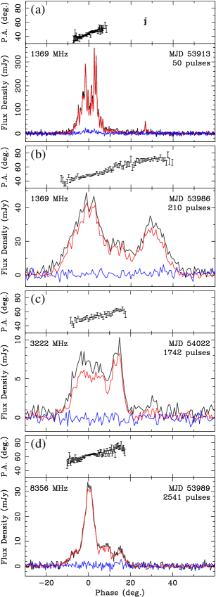
To complete polarization calibration for XTE J1810–197 we had to compute the amount of Faraday rotation suffered by the radiation in its passage through the Galactic magnetic field. We determined the rotation measure by measuring PA as a function of frequency within the 256-MHz band at 1.4 GHz when the pulsar was strong. The resulting value, $\mbox{RM}=+76\pm 4$ rad m^-2, did not vary within the quoted uncertainty either as a function of pulse phase or time. The RM was then used to correct the measured PAs and frequency-integrated $L$ at all frequencies to their values at infinite frequency so that a comparison could be made between frequencies (e.g., Karastergiou & Johnston, 2006). The PAs and $L$ shown in Figure 1 therefore represent those emitted at the pulsar. We also display in the Figure the Stokes $I$ and $V$ .

Together with the integrated column density of free electrons to XTE J1810–197, $\mbox{DM}=178$ cm^-3 pc (Camilo et al., 2006), the RM can be used to determine the average magnetic field strength parallel to the line of sight weighted by electron density, $1.2\,\mbox{RM/DM}=0.5\,\mu$ G. This fairly small value appears reasonable given the location of the pulsar, $(l,b)=(10\fdg 73,-0\fdg 16)$ and $d=3.5$ kpc, for which the large-scale Galactic field is mostly in the perpendicular direction, and with at least one reversal along the line of sight (e.g., Han et al., 2006).

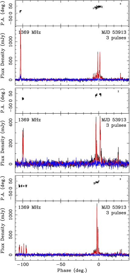
In spite of the variability of the profiles shown in Figure 1 there are three striking and constant aspects to the polarization profiles. First, the fractional linear polarization is extremely high, close to 100%, and remains high at all frequencies measured here¹¹1Camilo et al. (2006) reported that the pulsar was 65% linearly polarized at 1.4 GHz. The discrepancy arises from then-uncorrected Faraday rotation within the observing band.. Secondly, there is a shallow increase in the PA as a function of rotational phase, which remains essentially unchanged regardless of time or frequency of the observations. The rate of change is reasonably constant over the “main” pulse profile components and is around $0\fdg 5$ deg^-1. Finally, there is little or no circular polarization ( $\la 5\%$ ) in the integrated profiles at any frequency (Fig. 1), or in individual pulses at 1.4 GHz except for occasional levels up to $\sim 10\%$ of total intensity in the “precursor” pulse components (cf. Fig. 2).

The emission from XTE J1810–197 changed in character in late 2006 July (Camilo et al., 2007). While daily variations continue unabated, generally the pulse profiles are broader (compare Figs. 1 [a] and [b]) and the fluxes are lower (the peak flux densities listed in Table 1 attest to this). In contrast, the general polarization characteristics do not seem to vary. This suggests that the gross observed changes in profile morphology are not due to detectable changes in the underlying magnetic field geometry of the emission regions.

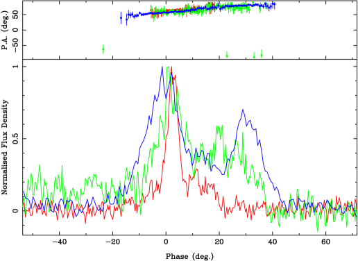
With the variability of the integrated profiles as a caveat, we nevertheless attempt to compare the profiles at 1.4, 3.2 and 8.4 GHz. In order to isolate long-term variations, we consider for this purpose only data taken in a one-week period in 2006 September. The double peaked profile gets narrower as the frequency increases and the ratio of the leading to trailing component becomes larger (Fig. 3). Also, the slow PA sweep (and absolute value of the PA) is identical at all frequencies, as expected in the “rotating vector model” of Radhakrishnan & Cooke (1969). This is consistent with the radius-to-frequency mapping paradigm in which lower frequencies are emitted farther from the star than higher frequencies (e.g., Cordes, 1978). Without detailed geometrical information, however, it is difficult to quantify this effect (for a brief discussion of radius-to-frequency mapping concerning XTE J1810–197, see Camilo et al., 2006; Dyks et al., 2007).

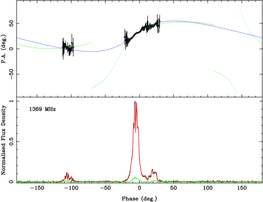
In the very early days of pulsar astronomy, it was realized that the observed PA swing could be used to derive the geometry of the star under the assumption that the PA was related to the projection of the dipolar field lines on the plane of the sky (Radhakrishnan & Cooke, 1969). Unfortunately, it is difficult to determine the geometry in the majority of pulsars mainly because of the small longitude range over which they emit (e.g., Everett & Weisberg, 2001). This is true of XTE J1810–197 also. In addition, it is a priori unclear whether a dipolar field structure holds true in this pulsar, although we proceed on the assumption that it might and see where that leads us. In our post-2006 July data, neither $\alpha$ (the angle between the magnetic and rotation axes) nor $\beta$ (the angle of closest approach of the line of sight to the magnetic axis) can be constrained. The earlier data, with the appearance of pulse components far from the main component (Fig. 2), are more promising in this regard. Here, however, the main uncertainty is whether there is 90\arcdeg of PA rotation between the widely spaced components. Formal fits to the data both with and without an extra 90\arcdeg of phase are reasonable (see Fig. 4). In the former case, the fits yield values of $\alpha$ near 70\arcdeg and high values of $\beta$ near 20\arcdeg–25\arcdeg. Without the added orthogonal jump, the fits yield $\alpha\sim 4\arcdeg$ and $\beta\sim 4\arcdeg$ implying that the magnetic and rotation axes are almost aligned.

The polarization characteristics of XTE J1810–197 are very similar to those seen in young pulsar profiles (Johnston & Weisberg, 2006). They too are highly linearly polarized, often have double profiles, and show a slow swing of PA across a wide profile. Johnston & Weisberg (2006) showed that a single cone of emission originating from relatively high in the pulsar magnetosphere could explain the observed characteristics of young pulsars and it is tempting to make the same case here. However, there is a significant difference in the polar cap radius, $\propto P^{-1/2}$ (and light cylinder radius $cP/2\pi$ ), between a young pulsar with a period of 0.1 s and XTE J1810–197 with its 5.5 s period. This makes it difficult to see how such a wide ( $\approx 0.15\,P$ ) observed pulse profile can be produced unless (a) the emission height is very large or (b) the magnetic and rotation axes are almost aligned. We will discuss these two possibilities in turn.

In the first case, knowledge of the geometry and the observed pulse width can be used to compute an emission height. For values of $\alpha$ near 70\arcdeg and $\beta\approx 25\arcdeg$ , one can use equation (2) of Gil et al. (1984) to derive the cone opening angle $\rho$ . In turn the emission height can be computed as $\sim 2cP\rho^{2}/9\pi$ , or $\sim 20000$ km. This is about 10% of the light cylinder radius — similar to the value in other young pulsars (Johnston & Weisberg, 2006). If this scenario were typical of magnetars in general then the beaming fraction would be high and most bright radio active magnetars would likely be detectable in pulsations. In the second case, for small values of $\alpha$ , the line of sight could remain wholly within the emission beam leading to the observed wide profile. In this case, if $\alpha$ were to vary slightly with time (for reasons unknown), there could be a large effect on both the observed beam shape and torque, both of which have been observed to vary significantly (Camilo et al., 2007). Perhaps the emission in this particular magnetar could be in part a direct function of the quasi-alignment between the rotation axis and magnetic axis, or perhaps the alignment might occur as a natural process in magnetars. In either case, the small polar cap size would make the beaming fraction of such magnetars rather low. The main difficulty with this interpretation is that the radio and X-ray beams appear to be nearly aligned (Camilo et al., 2007) and the observed modulation of thermal X-rays is very large ( $\sim 50\%$ ; Gotthelf & Halpern, 2007), which would be hard to obtain from a nearly aligned rotator.

In summary, the polarized emission from XTE J1810–197 shares many characteristics of those in young pulsars generally. The emission is highly linearly polarized with little evolution with frequency, the pulse profile is wide and double, and there is only a shallow swing of PA through the main pulse. This leads to the possibility that the “standard” pulsar ideas of emission along open magnetic field lines also hold here. In this case, either the magnetic and rotation axes are almost aligned, or the emission originates high above the surface of the star, which is our preferred interpretation. Obvious remaining differences between XTE J1810–197 and other pulsars are its pulse profile variability (which does not appear to be accompanied by corresponding gross changes in the magnetic field geometry), fluctuating flux density, and flat spectrum.

Acknowledgements.

We thank John Sarkissian for help with observations, and Aidan Hotan and Aris Karastergiou for discussions. The Parkes Observatory is part of the Australia Telescope, which is funded by the Commonwealth of Australia for operation as a National Facility managed by CSIRO. FC acknowledges the NSF for support through grant AST-05-07376.

References

Beloborodov & Thompson (2007) Beloborodov, A. M., & Thompson, C. 2007, ApJ, in press (astro-ph/0602417)
Camilo et al. (2007) Camilo, F., et al. 2007, ApJ, submitted (astro-ph/0610685)
Camilo et al. (2006) Camilo, F., Ransom, S. M., Halpern, J. P., Reynolds, J., Helfand, D. J., Zimmerman, N., & Sarkissian, J. 2006, Nature, 442, 892
Cordes (1978) Cordes, J. M. 1978, ApJ, 222, 1006
Duncan & Thompson (1992) Duncan, R. C., & Thompson, C. 1992, ApJ, 392, L9
Dyks et al. (2007) Dyks, J., Rudak, B., & Rankin, J. M. 2007, A&A, in press (astro-ph/0610883)
Everett & Weisberg (2001) Everett, J. E., & Weisberg, J. M. 2001, ApJ, 553, 341
Gil et al. (1984) Gil, J. A., Gronkowski, P., & Rudnicki, W. 1984, A&A, 132, 312
Gotthelf & Halpern (2005) Gotthelf, E. V., & Halpern, J. P. 2005, ApJ, 632, 1075
Gotthelf & Halpern (2007) Gotthelf, E. V., & Halpern, J. P. 2007, in Isolated Neutron Stars: From the Interior to the Surface, ed. S. Zane, R. Turolla, & D. Page, in press (astro-ph/0608473)
Halpern et al. (2005) Halpern, J. P., Gotthelf, E. V., Becker, R. H., Helfand, D. J., & White, R. L. 2005, ApJ, 632, L29
Han et al. (2006) Han, J. L., Manchester, R. N., Lyne, A. G., Qiao, G. J., & van Straten, W. 2006, Astrophys. J. , 642, 868
Hotan et al. (2004) Hotan, A. W., van Straten, W., & Manchester, R. N. 2004, Proc. Astr. Soc. Aust., 21, 302
Ibrahim et al. (2004) Ibrahim, A. I., et al. 2004, ApJ, 609, L21
Johnston (2002) Johnston, S. 2002, Proc. Astr. Soc. Aust., 19, 277
Johnston et al. (2005) Johnston, S., Hobbs, G., Vigeland, S., Kramer, M., Weisberg, J. M., & Lyne, A. G. 2005, MNRAS, 364, 1397
Johnston & Weisberg (2006) Johnston, S., & Weisberg, J. M. 2006, MNRAS, 368, 1856
Karastergiou & Johnston (2006) Karastergiou, A., & Johnston, S. 2006, MNRAS, 365, 353
Radhakrishnan & Cooke (1969) Radhakrishnan, V., & Cooke, D. J. 1969, Astrophys. Lett., 3, 225
Woods & Thompson (2006) Woods, P. M., & Thompson, C. 2006, in Compact Stellar X-ray Sources, ed. W. H. G. Lewin & M. van der Klis (Cambridge: CUP), 547–586

Refer to caption — Figure 1: Representative polarimetric profiles of XTE J1810–197 over time and frequency. The red and blue lines represent the amount of linear and circular polarization, respectively, and the black traces give total intensity. The position angles (PAs) are displayed for bins where the linear polarization signal-to-noise ratio $>4$ and have been corrected for rotation measure. In order to highlight the emission region, we show 90\arcdeg of pulse phase and a PA range of 30\arcdeg–90\arcdeg. Each data set was folded using a different ephemeris, and no attempt was made to align the panels precisely. Panel (a) shows a 5 min integration with 2048-bin resolution when the pulsar was strong (emission on this day was also detected at other phases; see Fig. 2). Panel (b) displays a 19 min integration when the pulsar had weakened and its profile had broadened considerably. Panel (c) shows a 2.7 hr integration, and (d) a 3.9 hr integration. Panels (b)–(d) are displayed with 512 bins across the full pulse period.