The ACS Virgo Cluster Survey. XII.
The Luminosity Function of Globular Clusters in Early Type Galaxies

Abstract

We analyze the luminosity function of the globular clusters (GCs) belonging to the early-type galaxies observed in the ACS Virgo Cluster Survey. We have obtained maximum likelihood estimates for a Gaussian representation of the globular cluster luminosity function (GCLF) for 89 galaxies. We have also fit the luminosity functions with an “evolved Schechter function”, which is meant to reflect the preferential depletion of low-mass GCs, primarily by evaporation due to two-body relaxation, from an initial Schechter mass function similar to that of young massive clusters in local starbursts and mergers. We find a highly significant trend of the GCLF dispersion $\sigma$ with galaxy luminosity, in the sense that the GC systems in smaller galaxies have narrower luminosity functions. The GCLF dispersions of our Galaxy and M31 are quantitatively in keeping with this trend, and thus the correlation between $\sigma$ and galaxy luminosity would seem more fundamental than older notions that the GCLF dispersion depends on Hubble type. We show that this narrowing of the GCLF in a Gaussian description is driven by a steepening of the cluster mass function above the classic turnover mass, as one moves to lower-luminosity host galaxies. In a Schechter-function description, this is reflected by a steady decrease in the value of the exponential cut-off mass scale. We argue that this behavior at the high-mass end of the GC mass function is most likely a consequence of systematic variations of the initial cluster mass function rather than long-term dynamical evolution. The GCLF turnover mass $M_{\rm TO}$ is roughly constant, at $M_{\rm TO}\simeq(2.2\pm 0.4)\times 10^{5}\,M_{\odot}$ in bright galaxies, but it decreases slightly (by $\sim\!35\%$ on average, with significant scatter) in dwarf galaxies with $M_{B,{\rm gal}}\gtrsim-18$. It could be important to allow for this effect when using the GCLF as a distance indicator. We show that part, though perhaps not all, of the variation could arise from the shorter dynamical friction timescales in less massive galaxies. We probe the variation of the GCLF to projected galactocentric radii of 20–35 kpc in the Virgo giants M49 and M87, finding that the turnover point is essentially constant over these spatial scales. Our fits of evolved Schechter functions imply average dynamical mass losses ($\Delta$) over a Hubble time that vary more than $M_{\rm TO}$, and systematically but non-monotonically as a function of galaxy luminosity. If the initial GC mass distributions rose steeply towards low masses as we assume, then these losses fall in the range $2\times 10^{5}\,M_{\odot}\lesssim\Delta<10^{6}\,M_{\odot}$ per GC for all of our galaxies. The trends in $\Delta$ are broadly consistent with observed, small variations of the mean GC half-light radius in ACSVCS galaxies, and with rough estimates of the expected scaling of average evaporation rates (galaxy densities) versus total luminosity. We agree with previous suggestions that if the full GCLF is to be understood in more detail, especially alongside other properties of GC systems, the next generation of GCLF models will have to include self-consistent treatments of dynamical evolution inside time-dependent galaxy potentials.

1. Introduction

One of the remarkable features of the systems of globular clusters (GCs) found around most galaxies is the shape of their luminosity function, or the relative number of GCs with any given magnitude. Historically most important has been the fact that these distributions always appear to peak, or turn over, at a GC absolute magnitude around $M_{V,{\rm TO}}\approx-7.5$ (e.g., Harris 2001), corresponding roughly to a mass of $M_{\rm TO}\sim 2\times 10^{5}\,M_{\odot}$. The near universality of this magnitude/mass scale for GCs has motivated the widespread use of the globular cluster luminosity function (GCLF) as a distance indicator (see Harris 2001; also Ferrarese et al. 2000), and it has also posed one of the longest-standing challenges to theories of GC formation and evolution.

In recent years, some significant amount of attention has also been paid to the way that GCs are distributed in mass around the peak of the GCLF. Traditionally, the full GCLF has most often been modeled as a Gaussian distribution in magnitude, corresponding to a lognormal distribution of GC masses. However, if one focuses only on the distribution of GCs above the point where the magnitude distribution turns over, it is found that the mass function can usually be described by a power law (Harris & Pudritz 1994), or perhaps a Schechter (1976) function (Burkert & Smith 2000), which is very similar to the mass distributions of giant molecular clouds and the young massive star clusters forming in starbursts and galaxy mergers in the local universe (e.g., Zhang & Fall 1999). The main difference between ancient GCs and the present-day sites of star-cluster formation is then that the mass functions of the latter rise steeply upwards towards masses much less than $M_{\rm TO}\sim\,10^{5}\,M_{\odot}$, far exceeding the observed frequency of such low-mass GCs.

There are two main possibilities to explain this fundamental difference. The first is that the conditions of star cluster formation in the early universe when GCs were assembling may have favored the formation of objects with masses in a fairly narrow range around $\sim\!10^{5}$–$10^{6}\,M_{\odot}$ (to the exclusion, in particular, of much smaller masses). These conditions would no longer prevail in the environments forming young clusters in the nearby universe. Some theoretical models along these lines invoke the $\sim\!10^{6}\,M_{\odot}$ Jeans mass at the epoch of recombination (Peebles & Dicke 1968), the detailed properties of $\sim\!10^{6}\,M_{\odot}$ cold clouds in a two-phase protogalactic medium (Fall & Rees 1985), and reionization-driven compression of the gas in subgalactic ($\lesssim\!10^{7}\,M_{\odot}$) dark-matter halos (Cen 2001).

The second possibility is that GCs were in fact born with a wide spectrum of masses, like that observed for young star clusters, extending from $\!10^{6}$–$10^{7}\,M_{\odot}$ down to $\sim\!10^{3}$–$10^{4}\,M_{\odot}$ or below. A subsequent transformation to the characteristic mass function of GCs today could then be effected mainly by dynamical processes (relaxation and tidal shocking) that are particularly efficient at destroying low-mass clusters over the lifetime of a GC system (e.g., Fall & Rees 1977; Ostriker & Gnedin 1997; Fall & Zhang 2001). Some observational evidence has been reported for such an evolution in the mass functions of young and intermediate-age star clusters (e.g., de Grijs, Bastian & Lamers 2003, Goudfrooij et al. 2004).

If we take the Occam’s-razor view that indeed GCs formed through substantially the same processes as star clusters today, then the picture offered by observations of old GCLFs is unavoidably one of survivors. There has been some debate as to whether it was in fact the long-term dynamical mechanisms just mentioned that were mainly responsible for destroying large numbers of low-mass globulars, or whether processes more related to cluster formation strongly depleted many low-mass protoclusters on shorter timescales (Fall & Zhang 2001; Vesperini & Zepf 2003). Even the most massive Galactic GCs have rather low binding energies $E_{b}\lesssim 10^{52}$ erg (McLaughlin 2000), so that if conditions were not just right, very many protoglobular clusters could have been easily destroyed in the earliest $\sim\!10^{7}$ yr of their evolution, through the catastrophic mass loss induced by massive-star winds and supernova explosions (see, e.g., Kroupa & Boily 2002; Fall, Chandar & Whitmore 2005). Furthermore, any clusters that survive this earliest mass-loss phase intact but with too low a concentration could potentially still dissolve within a relatively short time of $\sim\!10^{8}$–$10^{9}$ yr (Chernoff & Weinberg 1990). Homogeneous observations of large samples of old GCLFs can help clarify the relative importance of such early evolution versus longer-term dynamical mass loss in the lives of star clusters generally.

The largest previous studies of GCLFs in early-type galaxies were performed with archival HST/WFPC2 data. Kundu & Whitmore (2001a, b) studied the GCLF for 28 elliptical and 29 S0 galaxies. They concluded that the turnover magnitude of the GCLF is an excellent distance indicator, and that the difference in the turnover luminosity between the $V$ and $I$ bands increases with the mean metallicity of the GCs essentially as expected if the GC systems in most galaxies have similar age and mass distributions. Larsen et al. (2001) studied the GCLF for 17 nearby early-type galaxies. They fitted Student’s $t$ distributions separately to the subpopulations of metal-rich and metal-poor GCs in each galaxy, and found that any difference in the derived turnovers was consistent with these subpopulations having similar mass and age distributions and the same GCLF turnover mass scale. Larsen et al. also fitted power laws to the mass distributions of GCs in the range $M\simeq 10^{5}$–$10^{6}\,M_{\odot}$ and found they were well described by power-law exponents similar to those that fit the mass functions of young cluster systems.

In this paper, we study the GCLFs of 89 early-type galaxies observed by HST as part of the ACS Virgo Cluster Survey (Côté et al. 2004). This represents the most comprehensive and homogeneous study of its kind to date. Some of the results in this paper are also presented in a companion paper (Jordán et al. 2006). In the next section, we briefly describe our data and present our observed GCLFs in a machine-readable table available for download from the electronic edition of the Astrophysical Journal. In §3 we discuss two different models that we fit to the GCLFs, and in § 4 we describe our (maximum-likelihood) fitting methodology. Section 5 presents the fits themselves, while §6 discusses a number of trends for various GCLF parameters as a function of host galaxy luminosity and touches briefly on the issue of GCLF variations within galaxies. In §7 we discuss some aspects of our results in the light of ideas about GC formation and dynamical evolution, focusing in particular on the relation between our data and a model of evaporation-dominated GCLF evolution. In §8 we conclude.

2. Data

A sample of 100 early-type galaxies in the Virgo cluster was observed for the ACS Virgo Cluster Survey (ACSVCS; Côté et al. 2004). Each galaxy was imaged in the F475W ($\simeq$ Sloan $g$) and F850LP ($\simeq$ Sloan $z$) bandpasses for a total of 750 s and 1210 s respectively, and reductions were performed as described in Jordán et al. (2004a). These data have been used previously to analyze the surface-brightness profiles of the galaxies and their nuclei (Ferrarese et al. 2006ab, Côté et al. 2006), their surface brightness fluctuations (Mei et al. 2005ab; 2007), and the properties of their populations of star clusters, mainly GCs (Jordán et al. 2004b, Jordán et al. 2005, Peng et al. 2006a) but also dwarf-globular transition objects (or UCDs, Haşegan et al. 2005) and diffuse star clusters (Peng et al. 2006b).

One of the main scientific objectives of the ACSVCS is the study of the GC systems of the sample galaxies. We have developed a procedure by which we select GC candidates from the totality of observed sources around each galaxy, discarding the inevitable foreground stars and background galaxies that are contaminants for our purposes. This GC selection uses a statistical clustering method, described in detail in another paper in this series (Jordán et al. 2007, in preparation), in which each source in the field of view of each galaxy is assigned a probability $p_{\rm GC}$ that it is a GC. Our samples of GC candidates are then constructed by selecting all sources that have $p_{\rm GC}\geq 0.5$. The results of our classification method are illustrated in Figure 1 of Peng et al. (2006a). For every GC candidate we record the background surface brightness $I_{b}$ of the host galaxy at the position of the candidate, and we measure $z$- and $g$-band magnitudes and a half-light radius $R_{h}$ by fitting PSF-convolved King (1966) models to the local light distribution of the cluster (Jordán et al. 2005). Photometric zeropoints are taken from Sirianni et al. 2005 (see also Jordán et al. 2004a), and aperture corrections are applied as described by Jordán et al. (2007, in preparation).

Note that, as part of the ACSVCS we have measured the distances to most of our target galaxies using the method of surface brightness fluctuations (SBF; Tonry & Schneider 1988). The reduction procedures for SBF measurements, feasibility simulations for our observing configuration, and calibration have been presented in Mei et al. (2005ab) and the distance catalog is presented in another paper in this series (Mei et al. 2007). We use these distances in this paper to transform observed GC magnitudes into absolute ones on a per galaxy basis whenever we wish to assess GCLF properties in physical (i.e., mass-based) terms or need to compare the GCLFs of two or more galaxies. While some galaxies have larger distances, the average distance modulus that we employ is $(m-M)_{0}=31.09\pm 0.03\rm{(random)}\pm 0.15\rm{(systematic)}$, corresponding to $D=16.5\pm 0.1\rm{(random)}\pm 1.1\rm{(systematic)}$ Mpc.

2.1. GCLF Histograms

There are three main ingredients we need to construct a GCLF for any galaxy. First, we have sets of magnitudes, in both the $z$ and $g$ bands, for all GC candidates. As mentioned above, we generally isolate GC candidates from a list of all detected objects by requiring that $p_{\rm GC}\geq 0.5$. Note that here and throughout, we use $g$ as shorthand to refer to the F475W filter, and $z$ denotes F850LP. Also, all GC magnitudes in this paper have already been de-reddened (see § 2.7 in Jordán et al. 2004a for details).

Second, we have the (in)completeness functions in both bandpasses. Our candidate GCs are marginally resolved with the ACS, and thus these completeness functions depend not only on the GC apparent magnitude $m$ and its position in its parent galaxy (through the local background surface brightness $I_{b}$), but also on the GC projected half-light radius $R_{h}$. Separate $z$- and $g$-band completeness functions $f(m,R_{h},I_{b})\leq 1$ have therefore been calculated from simulations in which we first added simulated GCs with sizes $R_{h}=1,3,6,10$ pc and King (1966) concentration parameter $c=1.5$ to actual images from the ACSVCS (making sure to avoid sources already present), and then reduced the simulated images in an identical fashion to the survey data. We next found the fraction of artificial sources that were recovered, as a function of input magnitude and half-light radius, in each of ten separate bins of background light intensity. The final product is a three-dimensional look-up table on which we interpolate to obtain $f$ for any arbitrary values of $(m,R_{h},I_{b})$.

Last, we have the expected density of contaminants as a function of magnitude for each galaxy, obtained from analysis of archival ACS images (unassociated with the Virgo Cluster Survey) of 17 blank, high-latitude control fields, each observed with both $g$ and $z$ filters to depths greater than in the ACSVCS. We “customized” these data to our survey galaxies by performing object detections on every control field as if it contained each galaxy in turn. This procedure is described in more detail in Peng et al. (2006a, their §2.2). The net result is 17 separate estimates of the number of foreground and background objects, as a function of $g$ and $z$ magnitude, expected to contaminate the list of candidate GCs in every ACSVCS field.

Of the 100 galaxies in the ACSVCS, we restrict our analysis to those that have more than 5 probable GCs, as estimated by subtracting the total number of expected contaminants from the full list of GC candidates for each galaxy. We additionally eliminated two galaxies for which we could not usefully constrain the GCLF parameters. This results in a final sample of 89 galaxies. The GCLF data for these are presented in Table 1.

The first column of Table 1 is the galaxy ID in the Virgo Cluster Catalogue (VCC: Binggeli, Sandage & Tammann 1985; see Table 1 in Côté et al. 2004 for NGC and Messier equivalents). Column (2) contains an apparent $z$-band magnitude defining the midpoint of a bin with width $h_{z}$ given in column (3). This binwidth was chosen to be 0.4 for all galaxies. Columns (4)–(6) of the table then give the total number $N_{z,{\rm tot}}$ of observed sources in this bin; the number $N_{z,{\rm cont}}$ of contaminants in the bin as estimated from the average of our 17 control fields; and the average completeness fraction $f_{z}$ in the bin—all applying to the candidate-GC sample defined on the basis of our GC probability threshold, $p_{\rm GC}\geq 0.5$. Columns (7)–(11) repeat this information for the galaxy’s GC candidates identified in the $g$ band. Columns (12)–(21) are the corresponding $z$- and $g$-band data for an alternate GC sample defined strictly by magnitude cuts and an upper limit of $R_{h}<0\farcs 064\simeq 5$ pc (which will include the large majority of real GCs; Jordán et al. 2005), rather than by relying on our $p_{\rm GC}$ probabilities. This provides a way of checking that selecting GC candidates by $p_{\rm GC}$ does not introduce any subtle biases into the GCLFs (see also §4 below).

The data in Table 1 can be converted to distributions of absolute GC magnitude by applying the individual galaxy distances given in Mei et al. (2007). If they are used to fit model GCLFs, it should be by comparing the observed $N_{\rm tot}$ against a predicted $(f\times N_{\rm model}+N_{\rm cont})$ as a function of magnitude. This is essentially what we will do here, although we employ maximum-likelihood techniques rather than using the binned data. However, before describing our model-fitting methodology, we pause first to discuss in some detail the models themselves. We work with two different distributions in this paper: one completely standard, and one that is meant to elucidate the connections between observed GC mass distributions and plausible initial conditions and dynamical evolution histories.

3. Two GCLF Models

The term “globular cluster luminosity function” is customarily used to refer to a directly observed histogram of the number of GCs per unit magnitude. We follow this standard useage here, and in addition whenever we refer simply to a “luminosity function,” we in fact mean the GCLF, i.e., the distribution of magnitudes again. We denote the magnitude in any arbitrary bandpass by a lower-case $m$, and thus the GCLF is essentially the probability distribution function $dN/dm$. It is not equivalent to the distribution of true GC luminosities, since of course $m\equiv C-2.5\,\log\,L$ for some constant $C$, so $dN/dL=(dN/dm)|\partial m/\partial L|$ has a functional form different from that of $dN/dm$.

In this paper, when we speak of GC masses, we denote them by an upper-case $M$ and we almost always make the assumption that they are related by a multiplicative constant to GC luminosities, such that $m=C^{\prime}-2.5\,\log\,M$, with $C^{\prime}$ another constant including the logarithm of a mass-to-light ratio (generally taken to be the same for all GCs in any one system, as is the case in the Milky Way; McLaughlin 2000). We refer to the number of GCs per unit mass, $dN/dM$, as a “mass function” or a “mass distribution.” In the literature, it is sometimes also called a “mass spectrum.” Its relation to the GCLF is

$$\frac{dN}{dM}\propto\frac{1}{M}\frac{dN}{d\,\log\,M}\propto 10^{0.4m}\,\frac{dN}{dm}\ .$$ (1)

As we have already mentioned, most observed GCLFs show a “peak” or “turnover” at a cluster magnitude that is generally rather similar from galaxy to galaxy. One important consequence of equation (1) is that any such feature in the GCLF does not correspond to a local maximum in the GC mass distribution: if the first derivative of $dN/dm$ with respect to $m$ vanishes at some magnitude $m_{\rm TO}$, then the derivative of $dN/dM$ with respect to $M$ at the corresponding mass scale $M_{\rm TO}$ is strictly negative, i.e., the mass function still rises towards GC masses below the point where the GCLF turns over. (More specifically, the logarithmic slope of $dN/dM$ at the GCLF turnover point $M_{\rm TO}$ is always exactly $-1$; see McLaughlin 1994 for further discussion.)

3.1. The Standard Model

The function most commonly taken to describe GCLFs is a Gaussian, which is the easiest way to represent the peaked appearance of most luminosity functions in terms of number of clusters per unit magnitude. It is thus our first choice to fit to each of the observed GCLFs in this paper. Denoting the mean GC magnitude $\mu\equiv\langle m\rangle$ and the dispersion $\sigma_{m}=\langle(m-\mu)^{2}\rangle^{1/2}$, we have the usual

$$\frac{dN}{dm}=\frac{1}{\sqrt{2\pi}\,\sigma_{m}}\exp\left[-\frac{(m-\mu)^{2}}{2\sigma_{m}^{2}}\right]\ .$$ (2)

In terms of GC masses, $M$, this standard distribution corresponds to a mass function $dN/dM=(dN/dm)|\partial m/\partial M|$ or, since $m={\rm constant}-2.5\,\log\,M$ (assuming a single mass-to-light ratio for all clusters in a sample),

$$\frac{dN}{dM}=\frac{1}{(\ln 10)M}\frac{1}{\sqrt{2\pi}\,\sigma_{M}}\exp\left[-\frac{(\log\,M-\langle\log\,M\rangle)^{2}}{2\sigma_{M}^{2}}\right]\ ,$$ (3)

with $\sigma_{M}\equiv\sigma_{m}/2.5$.

As will be evident in what follows, the GCLFs in a large sample such as ours show a variety of detail that is unlikely to be conveyed in full by a few-parameter family of distributions. But it is also clear that a Gaussian captures some of the most basic information we are interested in investigating—the mean and the standard deviation of the GC magnitudes in a galaxy—with a minimal number of parameters. It is also the historical function of choice for GCLF fitting, and in many cases the fit is indeed remarkably good.

Nevertheless, the Gaussian does have some practical limitations. Secker (1992) showed that the tails of the GCLF in the Milky Way and M31 are heavier than a Gaussian allows, and he argued that a Student’s $t$ distribution (with shape parameter $\nu\simeq 5$) gives a better match to the data. More importantly, the observed GCLFs in our Galaxy and in M31 are asymmetric about their peak magnitude, a fact which has been emphasized most recently by Fall & Zhang (2001). This was implicit in the work of McLaughlin (1994), who advocated using piecewise power laws to fit the number of GCs per unit linear luminosity—or piecewise exponentials to describe the usual number of GCs per unit magnitude. Baum et al. (1997) used an asymmetric hyperbolic function to fit the strong peak and asymmetry in the combined Galactic and M31 GCLF.

However, all of these alternative fitting functions still share another shortcoming of the Gaussian, which is that there is no theoretical underpinning to it. Moreover, with the exception of the power laws in McLaughlin (1994), there is no obvious connection with the mass distributions of the young massive clusters that form in mergers and starbursts in the local universe. We therefore introduce an alternative fitting function—based on existing, more detailed studies of initial cluster mass functions and their long-term dynamical evolution—to address these issues.

3.2. An Evolved Schechter Function

3.2.1 Initial GC Mass Function

Observations of young star clusters indicate that the number of clusters per unit mass is well described by a power law—$dN/dM\propto M^{-\beta}$ with $\beta\approx 2$—or alternatively by a Schechter (1976) function with an index of about 2 in its power-law part and an exponential cut-off above some large mass scale that might vary from galaxy to galaxy (e.g., Gieles et al. 2006a). Perhaps the best-observed mass distribution for a young cluster system is that in the Antennae galaxies, NGC 4038/4039 (Zhang & Fall 1999). In this specific case, a pure power-law form suffices to describe the cluster $dN/dM$ as it is currently known; but a Schechter function with an appropriately high cut-off mass also fits perfectly well. Thus, assuming $dN/dM\propto M^{-\beta}\,\exp(-M/M_{c})$, we find from the data plotted by Zhang & Fall (1999) that $\beta=2.00\pm 0.04$ and $\log\,(M_{c}/M_{\odot})=6.3^{+0.7}_{-0.3}$ for their sample of clusters with ages 2.5–6.3 Myr; and $\beta=1.92\pm 0.14$ and $\log\,(M/M_{c})=5.9^{+0.45}_{-0.25}$ for ages 25–160 Myr.

The mass functions of old globular clusters in the Milky Way and M31 can also be described by power laws with $\beta\simeq 2$ for clusters more massive than the GCLF peak (McLaughlin 1994; McLaughlin & Pudritz 1996; Elmegreen & Efremov 1997). And the GC mass distributions in large ellipticals follow power laws over restricted high-mass ranges, although here the slopes are somewhat shallower (McLaughlin 1994; Harris & Pudritz 1994) and there is clear evidence of curvature in $dN/dM$ (McLaughlin & Pudritz 1996) that is better described by the exponential cut-off at very high cluster masses in a Schechter function (e.g., Burkert & Smith 2000). Theoretical models for GC formation, which aim expressly to explain these high-mass features of GCLFs and relate them to the distributions of younger clusters and molecular clouds, have been developed by McLaughlin & Pudritz (1996) and Elmegreen & Efremov (1997).

The important difference between the mass functions of old GCs and young massive clusters, then, is not the power-law or Schechter-function form of the latter per se; it is the fact that the frequency of young clusters continues to rise toward the low-mass limits of observations, while the numbers of GCs fall well below any extrapolated power-law behavior for $M\lesssim 2\times 10^{5}\,M_{\odot}$, i.e., for clusters fainter than the classic peak magnitude of the GCLF. We therefore assume a Schechter function,

$$\frac{dN}{dM_{0}}\propto M_{0}^{-2}\,\exp(-M_{0}/M_{c})\ ,$$ (4)

as a description of the initial mass distribution of globular clusters generally. We emphasize again that the fixed power law of $M_{0}^{-2}$ at low masses is chosen for compatibility with current data on systems of young massive clusters. The variable cut-off mass $M_{c}$ is required to match the well observed curvature present at $M\gtrsim 10^{6}\,M_{\odot}$ in the mass distributions of old GC systems in large galaxies. This feature is certainly allowed by the young cluster data, even if it may not be explicitly required by them.

A strong possibility to explain the difference between such an initial distribution and the present-day $dN/dM$ is the preferential destruction of low-mass globular clusters by a variety of dynamical processes acting on Gyr timescales (see Fall & Zhang 2001; Vesperini 2000, 2001; and references therein).

3.2.2 Evolution of the Mass Function

Fall & Zhang (2001) give a particularly clear recent overview of the dynamical processes that act to destroy globular clusters on Gyr timescales as they orbit in a fixed galactic potential. The main destruction mechanisms are dynamical friction; shock-heating caused by passages through galaxy bulges and/or disks; and evaporation as a result of two-body relaxation. Only the latter two are important to the development of the low-mass end of the GCLF, since dynamical-friction timescales grow rapidly towards low $M$, as $\tau_{\rm df}\propto M^{-1}$. (Cluster disruption due to stellar-evolution mass loss does not change the shape of the GC mass function if the stellar IMF is universal, unless a primordial correlation between cluster concentration and mass is invoked; cf. Fall & Zhang 2001 and Vesperini & Zepf 2003).

Tidal shocks drive mass loss on timescales $\tau_{\rm sh}\propto\rho_{h}P_{\rm cr}$, where $\rho_{h}\propto M/R_{h}^{3}$ is the mean density of a cluster inside its half-mass radius, and $P_{\rm cr}$ is the typical time between disk or bulge crossings. Evaporation scales rather differently, roughly as $\tau_{\rm ev}\propto M/\rho_{h}^{1/2}$. A completely general assessment of the relative importance of the two processes can therefore be complicated. However, tidal shocks are rapidly self-limiting in most realistic situations (Gnedin, Lee, & Ostriker 1999): clusters with high enough $\rho_{h}$ and on orbits that expose them only to “slow” and well-separated shocks (i.e., with both the duration of individual shocks and the interval $P_{\rm cr}$ longer than an internal dynamical time, $t_{\rm dyn}\propto\rho_{h}^{-1/2}$) will experience an early, sharp increase in $\rho_{h}$ in response to the first few shocks. Thereafter $\tau_{\rm ev}\ll\tau_{\rm sh}$, and in the long term shock-heating presents a second-order correction to the dominant mass loss caused by evaporation. Most GCs today, at least in our Galaxy, appear to be in this evaporation-driven evolutionary phase (Gnedin et al. 1999; see also Figure 1 of Fall & Zhang 2001, and Prieto & Gnedin 2006).

Fall & Zhang (2001) therefore develop a model for the evolution of the Galactic GCLF that depends largely on evaporation to erode an initially steep $dN/dM_{0}$ (in fact, they adopt a Schechter function, as in eq. [4], for one of their fiducial cases). They assume—as is fairly standard; e.g., see Vesperini (2000, 2001)—that any cluster roughly conserves its mean half-mass density $\rho_{h}$ as it loses mass, at least after any rapid initial adjustments due to stellar mass loss or the first tidal shocks, and when the evolution is dominated by evaporation. The mass-loss rate is then

$$\mu_{\rm ev}\equiv-dM/dt\propto M/t_{\rm rh}\propto(M/R_{h}^{3})^{1/2}\sim{\rm constant}\ ,$$ (5)

where $t_{\rm rh}\sim\rho^{-1}\langle v^{2}\rangle^{3/2}\propto M^{1/2}R_{h}^{3/2}$ is the relaxation time at the half-mass radius $R_{h}$. Under this assumption, the mass of a GC at any age $t$ is just $M(t)=M_{0}-\mu_{\rm ev}t$. For any collection of clusters with the same density (for example, those on similar orbits, if $\rho_{h}$ is set by tides at a well defined perigalacticon), $\mu_{\rm ev}$ is independent of cluster mass as well as time, and if the GCs are coeval in addition, then $\mu_{\rm ev}t$ is a strict constant. The mass function of such a cluster ensemble with any age $t$ is then related to the initial one as in equation (11) of Fall & Zhang (2001):

$$\frac{dN}{dM(t)}=\frac{dN}{dM_{0}}\left|\frac{\partial M_{0}}{\partial M}\right|=\frac{dN}{dM_{0}}\ .$$ (6)

Thus, simply making the substitution $M_{0}=M+\mu_{\rm ev}t$ in the functional form of the original GC mass function gives the evolved distribution. An initially steep $dN/dM_{0}$ therefore always evolves to a flat mass function, $dN/dM(t)\sim{\rm constant}$, at sufficiently low masses $M\ll\mu_{\rm ev}t$. As Fall & Zhang show for the Milky Way, and as we shall also see for the early-type ACSVCS galaxies, this gives a good fit to observed GCLFs if the cumulative mass-loss term $\mu_{\rm ev}t>10^{5}\,M_{\odot}$ by $t\simeq 13$ Gyr.

The key physical element of this argument, as far as the GCLF is concerned, is the linear decrease of cluster mass with time. While the quickest way to arrive at such a conclusion is to follow the logic of Fall & Zhang, as just outlined, there are some caveats to be kept in mind.

Tidal shocks can be much more important than evaporation for some globulars. In particular, clusters with low densities and low concentrations (such that shocks significantly disturb the cores as well as the halos), and/or those on eccentric orbits with very short intervals between successive bulge or disk crossings, may never recover fully from even one shock. Rather than re-adjusting quickly to a situation in which $\tau_{\rm ev}\ll\tau_{\rm sh}$, such clusters may be kept out of dynamical equilibrium for most of their lives, significantly overflowing their nominal tidal radii. Their entire evolution could then be strongly shock-driven. This appears to be the case, for example, with the well known Galactic globular, Palomar 5; see Dehnen et al. (2004). The extremely low mass and concentration of Palomar 5 make it highly unusual in comparison to the vast majority of known GCs in any galaxy currently, but many more clusters like its progenitor may well have existed in the past. This then raises the question of whether considering evaporation-dominated evolution alone gives a complete view of the dynamical re-shaping of the GC mass function. Here, however, it is important that the $N$-body simulations of Dehnen et al. (2004) show that the late-time evolution of even the most strongly shock-dominated clusters is still characterized by a closely linear decrease of mass with time: rather than $\rho_{h}$ being conserved in this case, the half-light radius $R_{h}$ is nearly constant in time, and for a given orbit the mass-loss rate is $M/\tau_{\rm sh}\propto M/\rho_{h}\propto R_{h}^{3}$. While the physical reasoning changes, the end result for the GCLF of clusters in this physical regime is the same as equation (6).

The importance of Fall & Zhang’s (2001) assumption of a constant $\rho_{h}$ for evaporation-driven cluster evolution is its implication that the mass-loss rate is constant in time. This has some direct support from N-body simulations (e.g., Vesperini & Heggie 1997; Baumgardt & Makino 2003). (Note the distinction in Baumgardt & Makino between the total cluster mass loss and that due only to evaporation; see their Figure 6 and related discussion.) But more than this, if evaporation is to be primarily responsible for the strong depletion of a GC mass function at scales $M<\mu_{\rm ev}t$, then after a Hubble time $\mu_{\rm ev}t$ must be roughly of order the current GCLF turnover mass $M_{\rm TO}\sim 2\times 10^{5}\,M_{\odot}$. Since $\mu_{\rm ev}\propto\rho_{h}^{1/2}$, this argument ultimately constrains the average density required of the globulars, which can of course be checked against data. In addition, satisfying observational limits on the (small) variation of GCLFs between different subsets of GCs in any one system—for example, as a function of galactocentric position—puts constraints on the allowed distribution of initial (and final) GC densities.

Fall & Zhang calculate in detail the evolution of the Milky Way GCLF over a Hubble time under the combined influence of stellar evolution (which, as mentioned above, does not change the shape of $dN/dM$ except in special circumstances), evaporation, and tidal shocks (which, again, contribute second-order corrections to the results of evaporation in their treatment). They relate $\mu_{\rm ev}\propto\rho_{h}^{1/2}$ to GC orbits, by assuming that $\rho_{h}$ is set by tides at the pericenter of a cluster orbit in a logarithmic potential with a circular speed of 220 km s^-1. They then find the GC orbital distribution that allows both for an average cluster density high enough to give a good fit to the GCLF of the Milky Way as a whole, and for a narrow enough spread in $\rho_{h}$ to reproduce the observed weak variation in $M_{\rm TO}$ with Galactocentric radius (e.g., Harris 2001).

Ultimately, the GC distribution function found by Fall & Zhang in this way is too strongly biased towards radial orbits with small pericenters to be compatible with the observed kinematics and $\rho_{h}$ distributions of globulars in the Milky Way and other galaxies—as both they and others (e.g., Vesperini et al. 2003) have pointed out. However, Fall & Zhang also note that the difficulties at this level of detail do not necessarily disprove the basic idea that long-term dynamical evolution is primarily responsible for the present-day shape of the GCLF at low masses. The problem may lie instead in the specific relation adopted to link the densities, and thus the disruption rates, of GCs to their orbital pericenters. In particular, Fall & Zhang—along with almost all other studies along these lines—assume a spherical and time-independent Galactic potential. Both assumptions obviously break down in a realistic, hierarchical cosmology. Once time-variable galaxy potentials are taken properly into account in more sophisticated simulations, it could still be found that cluster disruption on Gyr timescales can both explain the low-mass side of GC mass functions and be consistent with related data on the present-day cluster orbital properties, $\rho_{h}$ distributions, and so on. Recent work in this vein by Prieto & Gnedin (2006) appears promising, though it is not yet decisive.

We will return to these issues in §7.1. First, however, we describe an analytical form for $dN/dM$, which combines the main idea in Fall & Zhang (2001)—that evaporation causes cluster masses to decrease linearly with time—with a plausible, Schechter-function form for the initial $dN/dM_{0}$. We fit the evolved function to the GCLF of the Milky Way, to show that it provides a good approximation to the fuller, numerical models of Fall & Zhang; and then we fit it to our ACSVCS data, to produce new empirical constraints for detailed modeling of the formation and evolution of GC mass functions under conditions not specific only to our Galaxy.

3.2.3 Fitting Functions for $dN/dM$ and the GCLF

To summarize the discussion above, we assume that the mass-loss rate of any globular cluster is constant in time. Following Fall & Zhang (2001), we expect that this will occur naturally if the disruption process most relevant to the GCLF in the long term is evaporation, which plausibly conserves the average densities $\rho_{h}$ of individual clusters inside their half-mass radii. Thus, we continue to denote the mass-loss rate by $\mu_{\rm ev}$. However, it should be recognized that tidal shocks can contribute second-order corrections to $\mu_{\rm ev}$ and may even, in some extreme cases, dominate evaporation (though the net result arguably could still be a constant total $dM/dt$).

For any set of clusters with similar ages $t$ and similar $\rho_{h}$ (and on similar orbits, if these significantly affect $\rho_{h}$ or add tidal-shock contributions to $\mu_{\rm ev}$), the cumulative mass loss $\Delta\equiv\mu_{\rm ev}t$ is a constant, so that each cluster has $M(t)=M_{0}-\Delta$. Combining equation (4) for the initial mass distribution with equation (6) for its evolution then yields an “evolved Schechter function”

$$\frac{dN}{dM}\propto\frac{1}{(M+\Delta)^{2}}\,\exp\left(-\frac{M+\Delta}{M_{c}}\right)\ ,$$ (7)

with $M_{c}$ allowed to vary between galaxies. Once again, $\Delta$ in this expression may vary between different sets of GCs, with different densities or orbits, in the same galaxy. The detailed modeling of Fall & Zhang (2001) takes this explicitly into account. But in what follows, we fit equation (7) to GC data taken from large areas over galaxies, which effectively returns an estimate of the average mass loss per cluster over a Hubble time. Since $\mu_{\rm ev}\propto\rho_{h}^{1/2}$ when evaporation dominates shocks, this implicit averaging is essentially done over the distribution of GC mean half-mass densities.

To relate this evolved mass function to the standard observational definition of a GCLF—the number of GCs per unit magnitude—we write $m\equiv C-2.5\,\log\,M$, $\delta\equiv C-2.5\,\log\,\Delta$, and $m_{c}\equiv C-2.5\,\log\,M_{c}$, where $C$ is related to the solar absolute magnitude and the typical cluster mass-to-light ratio in an appropriate bandpass. The model then reads

$$\frac{dN}{dm}\propto\frac{10^{-0.4(m-m_{c})}}{\left[10^{-0.4(m-m_{c})}+10^{-0.4(\delta-m_{c})}\right]^{2}}\,\exp\left[-10^{-0.4(m-m_{c})}\right]\ .$$ (8)

In both of equations (7) and (8), the constants of proportionality required to normalize the distributions can be evaluated numerically.

Figure 1 illustrates the form of the evolved Schecter function, in terms of both the mass distribution $dN/dM$ and the GCLF $dN/dm$. (Note that mass $M$ increases to the right along the $x$-axis in the upper panel, but—as usual—larger $M$ corresponds to brighter magnitudes $m$, at the left of the axis in the lower panel.) From the equations above, it is clear that the mass $M_{c}$ or the magnitude $m_{c}$ sets the scale of the function, while the ratio $\Delta/M_{c}$ or the magnitude difference $(\delta-m_{c})$ controls its overall shape. For very small $\Delta\ll M_{c}$ (faint $\delta\gg m_{c}$), the function approaches an unmodified Schechter (1976) function. This is drawn in Figure 1 as the bold, broken curves that rise unabated toward low cluster masses or faint magnitudes. The magnitude $m_{\rm TO}$ at which the GCLF peaks in general can be found by setting to zero the derivative of equation (8) with respect to $m$. This yields

$$10^{-0.8(m_{\rm TO}-m_{c})}+10^{-0.4(m_{\rm TO}-m_{c})}\left[1+10^{-0.4(\delta-m_{c})}\right]-10^{-0.4(\delta-m_{c})}=0\ ,$$ (9)

the solution to which corresponds to a mass of

$$M_{\rm TO}=\frac{-(M_{c}+\Delta)+\sqrt{(M_{c}+\Delta)^{2}+4\Delta M_{c}}}{2}\ .$$ (10)

Figure 1.— Top: Evolved Schechter mass functions $dN/dM$ (eq. [7]), for various values of the ratio $\Delta/M_{c}$, which fixes the shape of the distribution. Curves are arbitrarily normalized. The uppermost, broken curve corresponds to $\Delta=0$, i.e., a regular Schechter (1976) function with a power-law exponent of $-2$. For non-zero $\Delta$, $dN/dM$ is flat at low masses. Bottom: GCLFs $dN/dm$ corresponding to the mass functions in the upper panel (see eq. [8]). Curves are again arbitrarily normalized, and the parameter controlling the shape is the magnitude difference $(\delta-m_{c})=-2.5\,\log(\Delta/M_{c})$. For any finite $(\delta-m_{c})$, the GCLF peaks and turns over at the magnitude $m_{\rm TO}$ given by equation (9) (corresponding to the mass in eq. [10]), and the faint side of the GCLF always approaches the limiting shape $dN/dm\propto 10^{-0.4m}$. Arrows mark the turnover points of the models shown here. In the limit $(\delta-m_{c})\rightarrow+\infty$ (i.e. $\Delta\ll M_{c}$), we have that $m_{\rm TO}\rightarrow\delta$, while in the limit $(\delta-m_{c})\rightarrow-\infty$ (large $\Delta\gg M_{c}$), the turnover $m_{\rm TO}\rightarrow m_{c}$. For $\Delta/M_{c}\gtrsim 10$ or $(\delta-m_{c})\lesssim-2.5$, the GCLF has an essentially fixed shape.

From either of equations (9) or (10), or from the sequence of curves in Figure 1, it can be seen that when $\Delta\ll M_{c}$, the GCLF peaks at a magnitude $m_{\rm TO}\simeq\delta$, i.e., the turnover reasonably approximates the average cluster mass loss in the model (although $m_{\rm TO}$ is formally always fainter than $\delta$). As the ratio $\Delta/M_{c}$ increases, the GCLF turnover initially tracks $\Delta$ but eventually approaches an upper limit set by the exponential cut-off scale in the mass function: $m_{\rm TO}\rightarrow m_{c}$ as $(\delta-m_{c})\rightarrow-\infty$ ($\Delta\gg M_{c}$).

For any fixed value of $\Delta/M_{c}$, Figure 1 shows that in the limit of low masses, $M\ll\Delta$, the mass function in equation (7) is essentially flat. As Fall & Zhang (2001) first pointed out, this is a direct consequence of the assumption of a mass-loss rate that is constant in time. It follows generically from equation (6) above, independently of the specific initial GC mass function. At the other extreme, for very high masses $M\gg\Delta$ the evolved $dN/dM$ just approaches the assumed underlying initial function with $\Delta=0$. In terms of the GCLF, this means that $dN/dm$ tends (always) to an exponential, $dN/dm\propto 10^{-0.4\,m}$, at magnitudes much fainter than the turnover; and (for initial Schechter function assumed here) to the steeper $dN/dm\propto 10^{0.4\,m}\exp\,[-10^{-0.4\,(m-m_{c})}]$ for very bright magnitudes. The faint half of the GCLF in this model is therefore significantly broader than the bright half.

Finally, it is worth considering the widths of the GCLFs in the lower panel of Figure 1 in more detail. For $\Delta=0$, the full width at half-maximum (FWHM) of $dN/dm$ is undefined, since there is no turnover. As the ratio $\Delta/M_{c}$ increases and a well-defined peak appears in the GCLF, the distribution clearly becomes narrower and narrower. As we have already discussed, even though formally $\Delta/M_{c}$ can increase without limit, the turnover magnitude ultimately has a maximum brightness $m_{\rm TO}\rightarrow m_{c}$. Similarly, the FWHM of the GCLF approaches a firm lower limit of ${\rm FWHM}\simeq 2.66$ mag. This includes a limiting half width at half-maximum of ${\rm HWHM}\simeq 1.59$ mag on the faint side of the GCLF, and a smaller ${\rm HWHM}\simeq 1.07$ mag on the bright side. All of these numbers can be obtained from analysis of equation (8) by letting $(\delta-m_{c})\rightarrow-\infty$, i.e., $\Delta/M_{c}\rightarrow+\infty$. In this limit, the GCLF approaches a fixed shape and is free only to shift left or right depending on the value of $m_{c}\simeq m_{\rm TO}$. This limiting shape is already essentially achieved with $\Delta/M_{c}=10$ or $(\delta-m_{c})=-2.5$, which is plotted in Figure 1 (even though the turnover is still about 0.18 mag fainter than $m_{c}$ in this case).

As we will see in §5.2 and §6.1.2, the GCLFs observed in the ACSVCS are all best fit with $\Delta/M_{c}\gtrsim 0.1$, or $(\delta-m_{c})\lesssim 2.5$ mag. This is the case also in the Milky Way.

3.3. Comparison with the Milky Way GCLF

Figure 2 plots the GCLF and the corresponding GC mass function in the Milky Way. The upper panel of this figure shows the GCLF $dN/dm$, in terms of clusters per unit absolute $V$ magnitude, for 143 GCs in the online catalogue of Harris (1996). (Note again that cluster luminosity and mass increase to the left in this standard magnitude distribution.) The bold, dashed line is the usual Gaussian representation (eq. [2]) with parameters given by Harris (2001):

$$\mu_{V}=-7.4\pm 0.1\ {\rm mag}\ ;\quad\sigma_{V}=1.15\pm 0.10\ {\rm mag}\ .$$ (11)

The bold solid curve is our fit of the evolved Schechter function in equation (8), with

$$\delta_{V}=-8.0\pm 0.3\ {\rm mag}\ ;\quad m_{c,V}=-9.3\pm 0.3\ {\rm mag}\ .$$ (12)

The lighter, broken line rising steeply towards faint magnitudes is a normal Schechter function with $m_{c}$ as in equation (12) but no mass-loss parameter, i.e., $\delta\rightarrow\infty$ in equation (8). The shape of this curve is therefore typical of the distribution of logarithmic mass for young massive clusters in nearby galaxies.

Figure 2.— Top: Fits of a Gaussian (dashed curve) and an evolved Schechter function (solid curve) to the Milky Way GCLF, expressed as the (normalized) number of clusters per unit of absolute $V$ magnitude. The dot-dashed curve is a Schechter function with the same value for $M_{c}$ as the solid curve but with mass-loss parameter $\Delta$ set to zero. Bottom: Corresponding observed GC mass function $dN/dM$, and model fits, derived from the GCLF assuming a $V$-band mass-to-light ratio of $2\ M_{\odot}\ L_{V,\odot}^{-1}$ for all clusters (McLaughlin & van der Marel 2005).

The lower panel of Figure 2 contains a log-log representation of the Galactic GC mass function, $dN/dM$. To construct this distribution, we converted the absolute $V$ magnitude of each GC into an equivalent mass by assuming a mass-to-light ratio of $\Upsilon_{V}=2\ M_{\odot}\,L_{\odot}^{-1}$ for all clusters (as implied by population-synthesis models; see McLaughlin & van der Marel 2005). The curves here are the mass equivalents of those in the upper panel. Thus the bold, dashed curve traces equation (3) with

$$\langle\log(M/M_{\odot})\rangle=5.2\pm 0.04\ ;\quad\sigma_{M}=0.46\pm 0.04$$ (13)

while the solid curve is equation (7) with

$$\log\,(\Delta/M_{\odot})=5.4\pm 0.1\ ;\quad\log\,(M_{c}/M_{\odot})=5.9\pm 0.1$$ (14)

and the lighter broken curve is equation (7) with $\log\,(M_{c}/M_{\odot})=5.9$ and $\Delta=0$—again, representative of young cluster mass functions.

Although both model fits to the GCLF are acceptable in a statistical sense, the evolved Schechter function yields a significantly lower $\chi^{2}$ value. This is because of the clear asymmetry in the observed GCLF, which appears as a faintward skew in the top panel and as a failure of the mass function $dN/dM$ to decline toward low masses in the bottom panel. This behavior is described well by the evolved Schechter function but is necessarily missed by the Gaussian, which systematically underestimates the number of clusters with $M\lesssim 3\times 10^{4}\,M_{\odot}$.

As a result of this, the best-fit evolved Schechter function yields a GCLF peak which is slightly brighter than the Gaussian. From the parameters given just above and either of equations (9) or (10), we find a turnover magnitude of $m_{\rm TO}=-7.5\pm 0.1$ in the $V$ band, some 0.1 mag brighter than the Gaussian turnover in equation (11). The turnover mass implied by the evolved Schechter function is thus $M_{\rm TO}\simeq(1.75\pm 0.15)\times 10^{5}\,M_{\odot}$, just over 10% more massive than the Gaussian fit returns. The intrinsically symmetric Gaussian model is forced to a fainter or lower-mass turnover in order to better fit the relatively stronger low-mass tail of the observed GCLF. We find similar offsets in general between the GCLF turnovers from the two model fits to our ACSVCS data (see §5 and §6 below).

We reiterate that the parameter $\Delta$ in the evolved Schechter function represents the average total mass loss per cluster (presumably due mostly to evaporation) that is required to transform an initial mass function like that of young clusters in the local universe, into a typical old GCLF. Both qualitatively and quantitatively, our model fits in Figure 2 correspond to the various similar plots in Fall & Zhang (2001). In fact, the value $\Delta\simeq(2.5\pm 0.5)\times 10^{5}\,M_{\odot}$ obtained here for the Milky Way agrees well with the mass losses required by Fall & Zhang for their successful models with the second-order effects of tidal shocks included. The simple function in equation (7) is thus a good approximation to their much fuller treatment of the GCLF.

It is also worth emphasizing just how close $\Delta$ is to the GCLF turnover mass scale. This implies that essentially all globulars currently found in the faint “half” of the GCLF are remnants of substantially larger initial entities. Equivalently, any clusters initially less massive than $\simeq\!2$–$3\times 10^{5}\,M_{\odot}$ are inferred to have disappeared completely from the GC system.

Despite any difficulties in detail (§3.2.2 and §7.1) that might remain to be resolved in this evaporation-dominated view of the GCLF, and of GC systems in general, it is important just to have at hand a fitting formula like the evolved Schechter function. In purely phenomenological terms, it fits the GCLF of the Milky Way—which is, after all, still the best defined over the largest range of cluster masses—at least as well as any other function yet tried in the literature. In particular, it captures the basic asymmetry of the distribution without sacrificing the small number of parameters and the simplicity of form that have always been the primary strengths of a Gaussian description. But at the same time, it is grounded in a detailed physical model with well specified input assumptions (Fall & Zhang 2001). Fitting it to large datasets, such as that afforded by the ACSVCS, thus offers the chance to directly, quantitatively, and economically assess the viability of these ideas, in much more general terms than has been possible to date.

4. Fitting Methodology and Technical Considerations

4.1. Maximum-Likelihood Fitting

Given either of the models just discussed—or, of course, any other—we wish to estimate a set of parameters for the intrinsic GCLF of a cluster sample using the method of maximum likelihood, following an approach similar to that of Secker & Harris (1993). To do so, we make use of all the observational material described in §2.1.

First, we denote the set of GC magnitudes and uncertainties in any galaxy, in either the $z$ or the $g$ band, by $\{m_{i},\epsilon_{m,i}\}$. Second, we write the three-dimensional completeness function discussed above as $f(m,R_{h},I_{b})$, which again depends not only on GC apparent magnitude but also on a cluster’s half-light radius and the background (“sky” and galaxy) light intensity at the position of the cluster. Third, from our 17 control fields we are able to estimate the luminosity function of contaminants in the field of any ACSVCS galaxy. We call this function $b(m)$, and we determine it by constructing a normal-kernel density estimate, with bandwidth chosen using cross-validation (see Silverman 1986, §§ 2.4, 3.4). Finally, this further allows us to estimate the net fractional contamination in the GC sample of each galaxy: $\widehat{\cal B}=N_{C}/N$, where $N_{C}\equiv(1/17)\sum_{i=1}^{17}N_{C,i}$ with $N_{C,i}$ the total number of contaminants present in the $i$-th customized control field, and $N$ is the total number of all GC candidates in the sample.

Now, given this observational input, we assume that an intrinsic GCLF is described by some function $G(m|\Theta)$, where $\Theta$ is the set of model parameters to be fitted. The choices for $G$ that we explore in this paper were discussed in detail in §3. Thus, for example, for the Gaussian model of equation (2), $\Theta\equiv\{\mu,\sigma_{m}\}$, while for the evolved Schechter function of equation (8), $\Theta\equiv\{\delta,m_{c}\}$. We further assume that magnitude measurement errors are Gaussian distributed, so that—in the absence of contamination—the probability of finding an apparent magnitude $m$ for a GC with given effective radius $R_{h}$, galaxy background $I_{b}$, and magnitude uncertainty $\epsilon_{m}$ would be

$$G_{T}(m|\Theta,R_{h},I_{b},\epsilon_{m})={\cal A}\ [h(m|\epsilon_{m})\otimes G(m|\Theta)]f(m,R_{h},I_{b}),$$ (15)

where $h(m|\epsilon_{m})=(2\pi\epsilon_{m}^{2})^{-1/2}\exp(-m^{2}/2\epsilon_{m}^{2})$; $\otimes$ denotes convolution; and the normalization ${\cal A}$—a function of the GCLF parameters $\Theta$ and the GC properties $R_{h}$, $I_{b}$, and $\epsilon_{m}$—is fixed by requiring that the integral of $G_{T}$ over the entire magnitude range covered by the observations be unity.

If a fraction ${\cal B}$ of sources in a galaxy are contaminants, then the probability of having a bona fide GC with magnitude $m$ (and given $R_{h}$, etc.) is reduced to $(1-{\cal B})G_{T}$, and thus the likelihood that a set of GCLF model parameters $\Theta$ can account for $N$ total objects with observed magnitudes $\{m_{i}\}$ and properties $\{R_{h,i},I_{b,i},\epsilon_{m,i}\}$ is

$${\cal L}(\Theta,{\cal B})=\prod_{i=1}^{N}\left[(1-{\cal B})G_{T}(m_{i}|\Theta,R_{h,i},I_{b,i},\epsilon_{m,i})+{\cal B}b(m_{i})\right]$$ (16)

in which it is assumed that the luminosity function $b(m)$ of contaminants is also normalized.

For any chosen functional form $G(m|\Theta)$ of the intrinsic GCLF, we specify some initial parameter values $\Theta$, compute $G_{T}$ and $b$ for each observed object in a galaxy, and maximize on $\Theta$ the product in equation (16). In principle, it is possible simultaneously to determine the contamination fraction in this way, but in practice we found this to be a rather unstable procedure (even small inadequacies in the chosen model for $G$ can lead to a maximum-likelihood solution that converges to quite unreasonable values for ${\cal B}$). Thus, we instead made direct use of our prior information from the 17 control fields, and fixed this fraction to the rather precise average $\widehat{\cal B}$ that we have measured for each galaxy.

The uncertainties in the fitted parameters $\Theta$ are estimated by using the covariance matrix calculated at the point of maximum likelihood (e.g., Lupton 1993). These uncertainties include the effects of possible correlation between the parameters, but they do not include the additional, unavoidable uncertainty arising from cosmic variance in the form of $b(m)$ and the expected number $\widehat{\cal B}$ of contaminants in any field. As such, they constitute lower limits to the total uncertainty. This is not a significant issue for GCLF fits to cluster samples combined from several galaxies (see below), but it can be important for fits to individual galaxies.

To deal with this, when we fit any individual GC system, we re-run our maximum-likelihood algorithm 17 times, each time using the background contamination fraction ${\cal B}$ as estimated from a different one of our 17 control fields (versus using $\widehat{\cal B}$ from an average of all control fields to obtain the nominal best fit). We record the different sets of best-fit GCLF parameters obtained in these trials and use the variance in them to evaluate the additional uncertainty arising from cosmic variance of the background contamination.

4.2. Bias Tests

Maximum-likelihood estimators are biased in general. It is thus important when deriving conclusions to test the bias properties of the estimator used, under circumstances similar to the ones under study. We have done this specifically for the benchmark case of Gaussian fits to the GCLF. After obtaining mean magnitudes and dispersions from our maximum-likelihood routine for the 89 ACSVCS galaxies, we analyzed 20 simulated datasets per galaxy, using the following procedure. First, we subtracted the number of contaminants $\widehat{\cal B}N$ in the galaxy from the total number $N$ of GC candidates there, to estimate the expected population $N_{\rm GC}$ of bona fide GCs. We then randomly drew a sample of $N_{\rm GC}$ magnitudes from a Gaussian distribution with a mean $\mu$ taken to be the fitted maximum-likelihood estimate for that galaxy, and a dispersion chosen from $\sigma_{m}=0.4,0.7,1$ or 1.3 mag. (We did 5 simulations for each of these dispersions, giving the total of 20 simulations per galaxy.) The randomly generated objects replaced the $N_{\rm GC}$ objects in that galaxy’s sample with the highest $p_{GC}$ values. The values of $R_{h}$ and $I_{h}$ of the latter objects plus the simulated magnitude are used to determine the completeness value $f$ for each source. A uniform random deviate is then computed and if that is larger than the value of $f$ the source is discarded, a new magnitude drawn from the Gaussian and the process repeated until the condition is met. In this way the effects of completeness are taken into account. The maximum-likelihood procedure was finally run on each simulated sample and the output parameters compared to the input ones.

The results of these simulations in the $z$ band are summarized in Figure 3. There may be slight biases in the recovered parameters, with $\langle\Delta\sigma_{m}/\sigma_{m}\rangle\approx\!-0.03$ and $\langle\Delta\mu/\sigma_{m}\rangle\approx\!-0.03$, although there are no significant trends in these average offsets with galaxy luminosity (i.e., sample size). Moreover, the statistical significance of these biases is not high ($<3\sigma$), and so we choose not to correct for them. As a result, it is possible that our output best-fit parameters are biased at the level of 3% of the GCLF dispersion; but with the possible exception only of the most populous GC system (that of M87=VCC 1316), this turns out always to be smaller than the formal uncertainties on the GCLF parameters (see §5.1). Note that the scatter of the retrieved parameters compared with the input ones increases towards fainter galaxy magnitudes because the candidate-GC sample size is decreasing, and the variance in the estimates of both $\sigma$ and $\mu$ scales as $\sim\!1/N$.

Figure 3.— Top: Fractional difference $\Delta\sigma_{z}/\sigma_{z}$ between input and recovered Gaussian dispersion for simulated GCSs with four different Gaussian dispersions assumed ($\sigma=0.4,0.7,1.0,1.3$). Bottom: Difference $\Delta\mu_{z}/\sigma_{z}$ between input and recovered Gaussian mean $\mu$ for the same simulated GCSs as in the upper panel.

4.3. Effects of Selection Procedure

As we mentioned in §2, the procedure we used to construct a sample of GC candidates for each galaxy involved assigning a probability $p_{\rm GC}$ to each source and allowing into the sample only those objects with $p_{\rm GC}\geq 0.5$. This may influence the resulting observed luminosity function and consequently affect the derived parameters of any fitted model. In order to check that we do not unduly bias our GCLF fitting by this selection technique, we also constructed alternate candidate-GC samples that do not use the selection on $p_{\rm GC}$ but only apply a magnitude cut and an upper limit of $R_{h}\lesssim 5$ pc (cf. the second half of Table 1 in §2.1). The magnitude distributions of such samples are free of any selection effects arising from using the $p_{\rm GC}$ values and are useful for testing the robustness of any result. Thus, when we fit GCLFs to any of our data, we have verified that consistent conclusions are obtained using either of our sample definitions.

4.4. Binned Samples

While we always perform GCLF fits to individual galaxies, some of the fainter systems suffer from small-number statistics and/or excessive contamination. We thus constructed still more GC samples by combining all candidate clusters from as many galaxies as required to reach a total sample size above some minimum. Going down the list of our target galaxies sorted by apparent $B$ magnitude, we accumulate galaxies until the expected number of bona fide GCs (i.e., the total number of candidates minus the number of contaminants estimated from our customized control fields) is $\gtrsim 200$. Although many of the brighter galaxies satisfy this condition by themselves, we refer to the samples defined in this way as “binned” samples. There are 24 of them in all, and they are used in §6 particularly, to assess trends in GCLF parameters as a function of galaxy luminosity without the significant scatter caused by the small numbers of GCs in faint systems.

Our SBF analysis has shown that some of the ACSVCS galaxies have distance moduli significantly different from the mean $(m-M)_{0}=31.09$ mag for Virgo (Mei et al. 2007), and thus simply combining the apparent magnitudes of GCs from different galaxies with no correction could artificially inflate the dispersion of any composite GCLF. To avoid this, we do the binning by first using the SBF distances to transform all candidate GC luminosities to the value they would have at a distance of 31.1 mag ($D=16.5$ Mpc).

5. Model Fits

In this section we present the results of our maximum-likelihood fitting of Gaussians and evolved Schechter functions to the GCLFs in the Virgo Cluster Survey. Recall that any alternative model may be fit to the GCLF histograms in Table 1, which can be downloaded from the electronic edition of the Astrophysical Journal.

5.1. Gaussian Fits

The parameter estimates for an intrinsic Gaussian fitted to our 89 individual GCLFs are given in Table 2. There we list each galaxy’s ID number in the VCC and its total apparent magnitude $B_{\rm gal}$, both taken from Binggeli, Sandage & Tammann (1985). Following this are the maximum-likelihood values of the mean GC magnitude and dispersion and their uncertainties in the $g$-band ($\mu_{g},\sigma_{g}$), the same quantities in the $z$-band ($\mu_{z},\sigma_{z}$), the fraction $\widehat{\cal B}$ of the sample that is expected to be contamination, and the total number $N$ of all objects (including contaminants and uncorrected for incompleteness) in the galaxy’s candidate-GC sample. The last column of Table 2 gives comments on a few galaxies with noteworthy aspects. Note that the uncertainties in the Gaussian parameters include contributions from cosmic variance in the shape and normalization of the contamination luminosity function $b(m)$ (see §4.1).

In Figure 4 we present histograms of the observed GCLFs along with the best fitting maximum-likelihood models. The galaxies are arranged in order of decreasing apparent $B_{\rm gal}$ magnitude (i.e., the same order as in Table 2), and there are two panels per galaxy: one presenting the $z$-band data and model fits, and one for the $g$ band. The bin width chosen for display purposes here is not the same for all galaxies, but follows the rule $h=2(IQR)N^{-1/3}$, where $(IQR)$ is the interquartile range of the magnitude distribution and $N$ is the total number of objects in each GC sample (Izenman 1991).

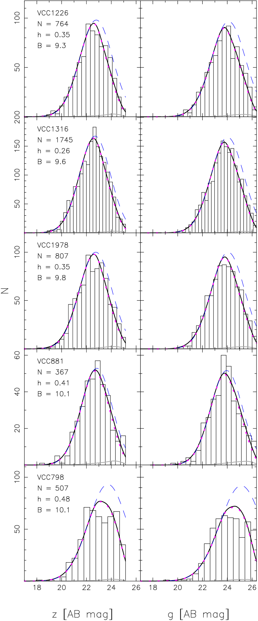
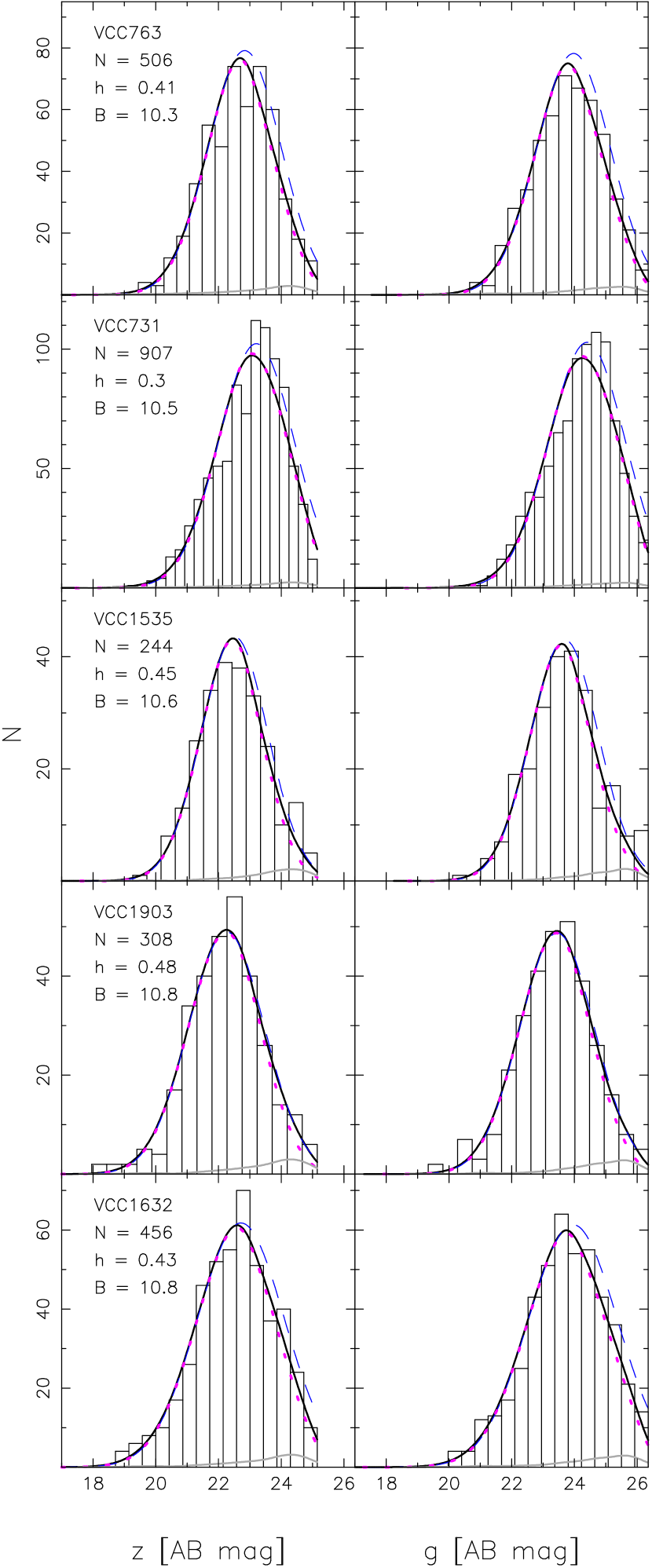
Figure 4.— Histograms of the GCLFs for our sample galaxies. For each galaxy we present the $z$-band and $g$-band GCLFs side by side. The VCC name and $B$ magnitude of the galaxy are indicated in the upper left corner of the left panel, where we also indicate the total number of sources in each histogram and the bin-width $h$ used to construct the histogram. Additionally we show the best-fit model (solid black curve), the intrinsic Gaussian component (dashed curve), the Gaussian component multiplied by the expected completeness (dotted curve) and a kernel-density estimate of the expected contamination in the sample (solid gray curve). The solid black curve is the sum of the solid gray and dotted curves. The galaxies are ordered by decreasing apparent $B$-band total luminosity, reading down from the upper left-hand corner. The parameters of the fits are given in Table 2.

Fig. 4. — Continued

Fig. 4. — Continued

Fig. 4. — Continued

Fig. 4. — Continued

Fig. 4. — Continued

Fig. 4. — Continued

Fig. 4. — Continued

Fig. 4. — Continued

There are four curves drawn in every panel of Figure 4. The long-dashed curve is the best-fit intrinsic Gaussian GCLF, given by equation (2) with the parameters listed in Table 2. The dotted curve is this intrinsic model multiplied by the completeness function, $f(m,R_{h},I_{b})$, after marginalizing the latter over the distribution of $R_{h}$ and $I_{b}$ for the observed sources in each galaxy. The solid gray curve is our kernel-density estimate of the expected contaminant luminosity function. Finally, the solid black curve is the sum of the solid gray and dotted curves; it is the net distribution for which the likelihood in equation (16) above is maximized.

Since we have two realizations of the GCLF for every galaxy—one in the $z$ band and one in the $g$ band—we are able to check the internal consistency of our model parameter estimates. Thus, in Figure 5 we compare the measured Gaussian means and dispersions in the two bands. The left-hand panel of this plot shows the scatter of $\sigma_{z}$ vs. $\sigma_{g}$ about a line of equality, while the right-hand panel shows the difference in fitted means $(\mu_{g}-\mu_{z})$ vs. the average GC $(g-z)$ color in each galaxy (from Peng et al. 2006a), again compared to a line of equality. Both cases show excellent agreement between the maximum-likelihood results for the two bandpasses. We conclude that the measurements are internally consistent and that our uncertainty estimates are reasonable.

Figure 5.— (Left) Estimate of Gaussian dispersion in the $z$-band, $\sigma_{z}$, versus the same quantity in the $g$-band, $\sigma_{g}$, for the GCLFs of our sample galaxies. Uncertainties are 1$\sigma$. The line marks the one-to-one correspondence between these two quantities. (Right) Difference between estimates of Gaussian means in the $g$- and $z$-bands, $\mu_{g}-\mu_{z}$, versus the mean color $\langle g-z\rangle$ of the GC systems of our sample galaxies. Uncertainties are 1$\sigma$. The line marks the one-to-one correspondence between these two quantities.

Finally, we also fit Gaussians to our 24 “binned” GC samples, constructed by combining the candidates in as many galaxies as necessary to reach net sample sizes of at least 200 (see §4.4). The IDs and total magnitudes of the galaxies going into each of these bins are summarized in Table 3, along with the best-fit $z$- and $g$-band Gaussian parameters for each binned GCLF and the best-fit parameters for the evolved Schechter function discussed in §3 (see just below). In Figure 6 we display the binned GCLFs in histogram format, along with a number of curves representing the maximum-likelihood Gaussian fits. The curves in every panel have exactly the same meaning as in the individual GCLF fits of Figure 4. We additionally show in this Figure (as the crosses in each magnitude bin of each histogram) alternative GCLFs for the binned-galaxy samples, obtained by defining GCs on the basis of absolute magnitude and an upper limit on the half-light radius $R_{h}$ (§4.3).

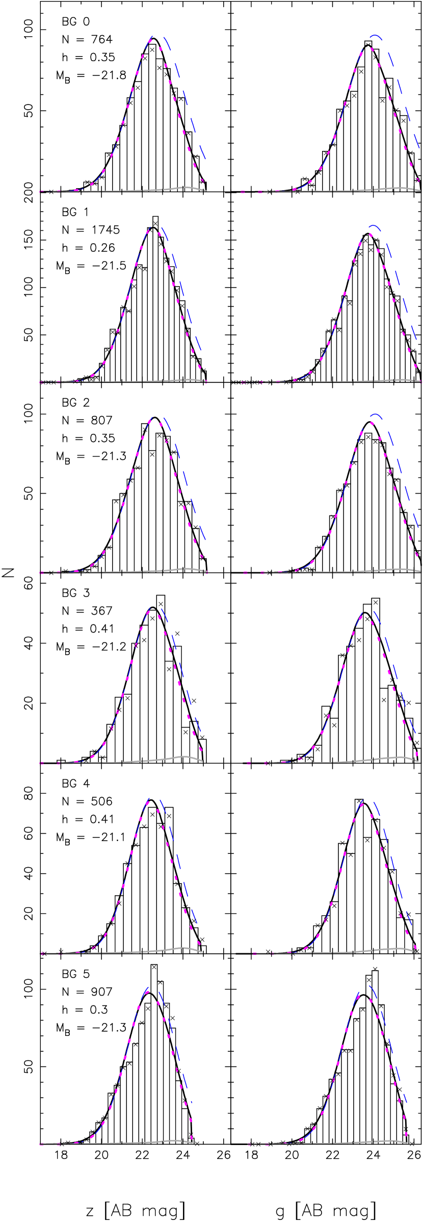
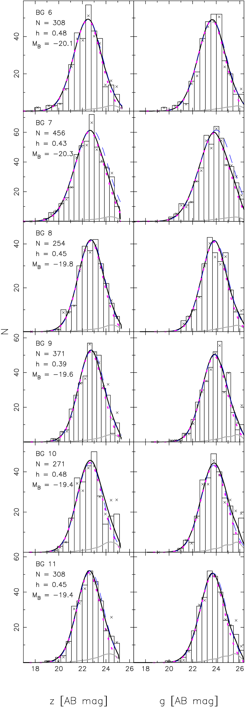
Figure 6.— Histograms and Gaussian fits to the GCLFs for our binned-galaxy samples. For each sample, named BG$n$ with $n=0,\ldots,23$, we present the $z$-band and $g$-band GCLFs side by side. The identifier of the galaxy bin is indicated in the upper left corner of the left panel, where we also indicate the number $N$ of all sources in the histogram (as chosen by requiring $p_{\rm GC}\geq 0.5$) and the bin-width $h$ used when constructing the histograms. In each panel we show the best fitting model (solid black curve), the intrinsic Gaussian component (dashed curve), the Gaussian component multiplied by the completeness fraction (dotted curve) and a kernel-density estimate of the expected contamination in the sample (solid gray curve). The solid black curve is the sum of the solid gray and dotted curves.The galaxy bins are ordered by decreasing mean apparent $B$-band luminosity of the galaxies that went into the sample construction. Crosses in all panels show the histograms that result when GC candidates are selected on the basis of cuts in magnitude and half-light radius; see §4.3. The parameters of all fits are given in Table 3.

Fig. 6. — Continued

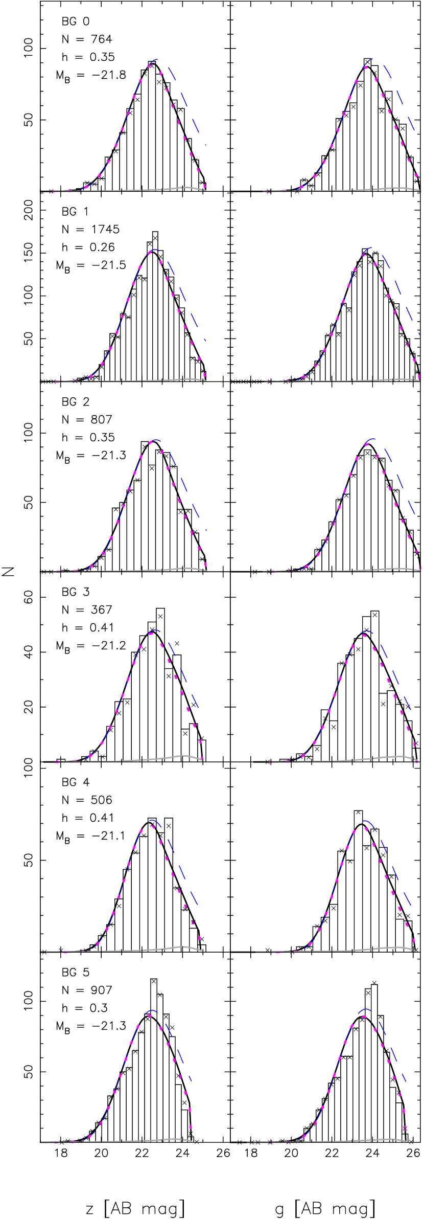
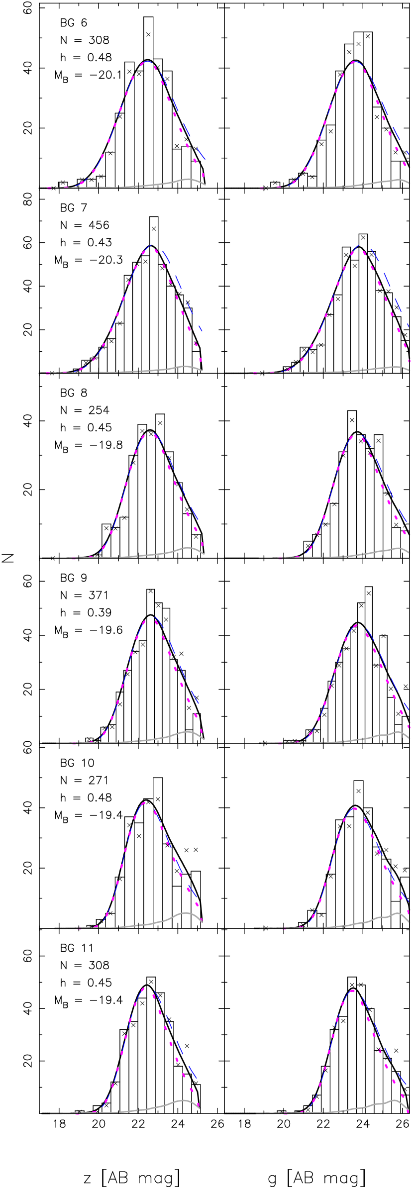
Figure 7.— Histograms and evolved Schechter function fits to the GCLFs for our binned-galaxy samples. For each sample, named BG$n$ with $n=0,\ldots,23$, we present the $z$-band and $g$-band GCLFs side by side. The identifier of the galaxy bin is indicated in the upper left corner of the left panel, where we also indicate the number $N$ of all sources in the histogram (as chosen by requiring $p_{\rm GC}\geq 0.5$) and the bin-width $h$ used when constructing the histograms. In each panel we show the best fitting model (solid black curve), the intrinsic evolved Schechter component (dashed curve), the evolved Schechter component multiplied by the completeness fraction (dotted curve) and a kernel-density estimate of the expected contamination in the sample (solid gray curve). The solid black curve is the sum of the solid gray and dotted curves. The galaxy bins are ordered by decreasing mean apparent $B$-band luminosity of the galaxies that went into the sample construction. Crosses in all panels show the histograms that result when GC candidates are selected on the basis of cuts in magnitude and half-light radius; see §4.3. The parameters of all fits are given in Table 3.

Fig. 7. — Continued

In §6 below, we will compare GCLF systematics as a function of galaxy properties for these binned samples vs. the fits to individual galaxies. We also note here, without showing further details, that repeating the exercises of this Section using the samples of GC candidates selected only by magnitude and $R_{h}$, rather than by a $p_{\rm GC}$ criterion, leads to results that are consistent in all ways with those we present below.

5.2. Fits of Evolved Schechter Functions

We have performed fits of the evolved Schechter function in equation (8)—or equivalently, the more transparent equation (7)—to the GCLFs of our individual galaxies and binned samples. Here we discuss only the results of fitting the 24 binned GC samples, as the results from fitting to all 89 galaxies separately lead to similar conclusions.

In all these fits, we enforced the constraint that the fitted (average) mass loss $\Delta$ be less than ten times the exponential cut-off mass scale $M_{c}$: $\Delta/M_{c}<10$, or $(\delta-m_{c})>-2.5$ in magnitude terms. This was done because, as was discussed in §3.2 (see Figure 1), for such large ratios of $\Delta$ to $M_{c}$ the evolved Schechter function has essentially attained a universal limiting shape. The likelihood surface then becomes very flat for any greater $\Delta/M_{c}$, and the fitting procedure has difficulty converging if this parameter is allowed to vary to arbitrarily high values. The majority of our evolved Schechter function fits do converge to $\Delta/M_{c}$ values that satisfy our imposed constraint; in only one case does the “best-fit” model have the limiting $\Delta/M_{c}=10$.

We show in Figure 7 the binned-sample GCLF histograms, along with model curves analogous to those in Figure 6. Again, then, the intrinsic evolved-Schechter model GCLF is the long-dashed curve; this model multiplied by the marginalized completeness function is the dotted curve; a kernel-density estimate of the contaminant luminosty function is shown as the solid gray curve; and the net best-fitting model (sum of dotted and solid gray curves) is drawn as a solid black curve. Also as in Figure 6, we use crosses in Figure 7 to show the GCLFs inferred in every galaxy bin when we define GC samples by simple magnitude cuts and $R_{h}$ limits, rather than by using our $p_{\rm GC}$ probabilities.

Comparing Figure 7 with Figure 6, it is apparent that an evolved Schechter function describes the GCLFs of bright galaxies about as well as a Gaussian does. In some of the fainter galaxies there is possibly a tendency for the Schechter function to overestimate the relative number of faint GCs, but it is difficult to assess how serious this might be. The worst disagreements between the model fits and the data tend to occur in the very faintest extents of the histograms for the handful of the faintest galaxy bins at the end of Figure 7. Indeed, the largest discrepancies appear at magnitudes where contaminants account for $\gtrsim 50\%$ of the total observed population. Any impression of success or failure for any model in these extreme regimes of the GCLFs must be tempered by the realization that the fitting itself is something of a challenge under such conditions.

This is further illustrated by contrasting, in both Figures 7 and 6, the GCLFs for cluster samples selected by magnitude and $R_{h}$ only (crosses in the figures), to those for samples selected on the basis of $p_{\rm GC}$ probabilities (bars). The former samples generally tend to put more objects in the faintest GCLF bins, an effect particularly apparent in the faintest galaxies. The low-mass end of the GCLF for faint galaxies is thus not tightly constrained by our observations; there is a fundamental uncertainty, due to contamination, that cannot be overcome by any selection procedure. (Note that some of the more extreme discrepancies between the different GCLF definitions—such as in the faintest magnitude bin of BG 20—are due to the presence in some galaxies of a strong excess of diffuse clusters that are classified as contaminants when using $p_{\rm GC}$ to construct the sample; see Peng et al. 2006b). But it is still worth recalling, in this context, that the “overabundance” of low-mass clusters in the evolved Schechter function, vs. a Gaussian, is in fact a demonstrably better description of the Milky Way GCLF; see Figure 2.

The fitted magnitude-equivalents $\delta$ and $m_{c}$ of the mass scales $\Delta$ and $M_{c}$, in each of the $z$ and $g$ bands, are recorded for each of our binned GCLFs in Table 3. In §6 we discuss in detail the conversion of these to masses and also consider dependences of $\Delta$ and $M_{c}$ on galaxy luminosity.

Just before looking at these issues, Figure 8 compares the turnover magnitudes and full-widths at half maximum (FWHM) for the binned $z$-band GCLFs as returned by the fits of evolved Schechter functions (see eq. [9]), against the same quantities implied by our Gaussian fits. For the turnovers, there is a slight offset, in that the fitted Schechter functions tend to peak at slightly brighter magnitudes (typical difference $\lesssim\!0.1$ mag, corresponding to a turnover mass scale that is $<\!10\%$ larger than implied by the Gaussian fits). This is very similar to the offset in the two fitted turnover magnitudes for the Milky Way GCLF in §3.3. As we discussed there, the discrepancy is a result of the intrinsic symmetry assumed in the Gaussian model, vs. the faint-end asymmetry built into the evolved Schechter function.

Figure 8.— Upper panel: Comparison of the absolute $z$-band magnitude of the GCLF turnover, as inferred from the maximum-likelihood fitting of intrinsic evolved Schechter functions versus that inferred from Gaussian fits. Lower panel: Comparison of the FWHM of the intrinsic $z$-band GCLFs, as returned by the Gaussian and evolved Schechter fits. Similar plots for the fits to our $g$-band GCLFs look the same as these $z$-band results.

The FWHMs differ more substantially between the two functional forms, with the evolved-Schechter fits being typically $\simeq\!0.5$ mag broader (or about 0.2 dex in terms of mass) than the Gaussian fits. But this is again only to be expected from the asymmetry of the former function vs. the symmetry of the Gaussian. As was noted at the end of §3.2, the shape of the evolved Schechter function is universally flat in terms of $dN/dM$ for low GC masses, or universally $\propto\!10^{-0.4m}$ in terms of $dN/dm$ for magnitudes much fainter than the peak of the GCLF. As a result, the faint side of the GCLF is always broader than any Gaussian, and so if the two models give comparable descriptions of the bright halves of all GCLFs, the FWHM of the evolved Schechter functions must always be larger than those of the Gaussian fits. Moreover, for very narrow observed GCLFs, fit by small Gaussian $\sigma_{m}$ (primarily to reproduce the steepness of the bright side of the GCLF, as discussed below), the evolved Schechter function fits are limited by a minimum FWHM of $\simeq\!2.66$ mag (§3.2), explaining the tendency towards a plateau at the left side of the lower panel of Figure 8.

6. Trends Between and Within Galaxies

Having fitted two different GCLF models to each of our individual galaxies and binned samples, we now outline some systematic variations in the properties of GC mass distributions indicated by this work. First, we examine the dependence of GCLF parameters on host galaxy luminosity; then—even though the ACSVCS data are not ideal for this purpose—we look for any evidence of GCLF trends with radius inside the two brightest Virgo galaxies, M49 (VCC 1226) and M87 (VCC 1316).

6.1. Variations with Galaxy Luminosity

6.1.1 Gaussian Parameters

Figure 9 shows one of the main results of this paper: GCLFs are narrower in lower-luminosity galaxies (see also Jordán et al. 2006).

Figure 9.— Top: GCLF dispersion $\sigma_{z}$, inferred from Gaussian fits to the $z$-band data, versus galaxy $M_{B,{\rm gal}}$. Filled symbols are galaxies for which we have available SBF distances while open triangles represent galaxies for which we do not and for which we have assumed a distance modulus of $(m-M)_{0}=31.1$. The dashed line is the linear relation between $\sigma_{z}$ and $M_{B,{\rm gal}}$ in equation (17). Bottom: Same comparison, but for the intrinsic Gaussian dispersion of the $g$-band GCLFs, $\sigma_{g}$. Dashed line is equation (18). In both panels the star shows values for the MW and the triangle represents M31. The outliers at $M_{B,\rm gal}\simeq-21.2$ and $M_{B,\rm gal}\simeq-19.9$ in both panels are VCC 798 and VCC 2095, galaxies which have an excess of faint, diffuse star clusters (Peng et al. 2006b).

The upper panel of this figure plots the Gaussian dispersion that best fits the $z$-band GCLF, as a function of absolute galaxy magnitude $M_{B,{\rm gal}}$ for our 89 individual galaxies. Filled circles represent galaxies with measured (SBF) distance moduli, while open triangles correspond to galaxies for which no distance modulus is available and for which we assume $(m-M)_{0}=31.1$ (consistent with the average Virgo distance modulus of Mei et al. 2007) to compute $M_{B,{\rm gal}}$. The lower panel shows the analogous result for our $g$-band GC data. The straight lines drawn in the panels are convenient linear characterizations of the $\sigma_{m}$–$M_{B,{\rm gal}}$ trends:

$$\sigma_{z}=(1.12\pm 0.01)-(0.093\pm 0.006)(M_{B,{\rm gal}}+20)$$ (17)

and

$$\sigma_{g}=(1.14\pm 0.01)-(0.100\pm 0.007)(M_{B,{\rm gal}}+20).$$ (18)

While it has been reported before that there is a tendency for the GCLFs in lower luminosity galaxies to show somewhat lower dispersions (e.g., Kundu & Whitmore 2001a), the homogeneity of our sample and analysis make this the most convincing demonstration to date of the existence of a continous trend over a factor of $\approx\!400$ in galaxy luminosity. It is particularly noteworthy that the fainter galaxies in our sample—all of which are early type—have very modest $\sigma_{m}\lesssim 1$, values more usually associated with the GCLFs of late-type galaxies. In fact we have also plotted on Figure 9 the $V$-band GCLF dispersions (Harris 2001) and absolute bulge luminosities of the Milky Way (large filled star at $M_{B,{\rm gal}}=-18.8$; de Vaucouleurs & Pence 1978) and M31 (large filled triangle at $M_{B,{\rm gal}}=-19.2$; from Kent 1989, but assuming a distance of 810 kpc). Clearly these fall well in the midst of our new data, and thus the correlation of $\sigma$ with $M_{B,{\rm gal}}$ would appear to be more fundamental than the older view, that GCLF dispersions depend on galaxy Hubble type (Harris 1991).

At this point it should be noted that the GCs in brighter galaxies are known to have broader color distributions, and hence larger dispersions in metallicity, than those in fainter galaxies (e.g., Peng et al. 2006a). But cluster mass-to-light ratios, $\Upsilon$, are functions of [Fe/H] in general, so there will be some galaxy-dependent spread in their values. Since the variance in an observed luminosity distribution is related to that in the mass distribution, by the usual $\sigma^{2}(\log\,L)=\sigma^{2}(\log\,M)+\sigma^{2}(\log\,\Upsilon)$, this then suggests the possibility that the trend we see in the GCLF $\sigma_{z}$ and $\sigma_{g}$ vs. galaxy luminosity might result from systematics in $\sigma(\log\,\Upsilon)$ vs. $M_{B,{\rm gal}}$ on top of a more nearly constant $\sigma(\log\,M)$. In fact, this idea was recently invoked by Waters et al. (2006) as a potential explanation for the fact that the $I$-band GCLF of M87 is broader than that of the Milky Way; and by Strader et al. (2006) as a possible reason for the narrower composite GCLF of a subsample of ACSVCS dwarfs versus the GCLFs of Virgo giants. However, neither of those works checked these claims quantitatively. We have done so here (see also Jordán et al. 2006), and we find that the explanation is not tenable.

As we will discuss further in §6.1.2, GC mass-to-light ratios in the longer-wavelength $z$ band vary by less than $\pm 10\%$ over the entire range $-2\leq{\rm[Fe/H]}\leq 0$, which includes the large majority of clusters. Thus $\sigma(\log\,\Upsilon_{z})<0.04$ no matter what the details of the GC metallicity distribution are—making for an utterly negligible “correction” to the observed $\sigma(\log\,L_{z})=\sigma_{z}/2.5$ for all of our GCLFs. In the shorter-wavelength $g$ band, mass-to-light ratios are more sensitive to cluster colors. But here the close agreement of our $g$- and $z$-band GCLF dispersions shows immediately that the former must be reflecting the properties of the GC mass functions just as closely as the latter are. Indeed, more detailed calculations, which include the observed specifics of the color distributions in our galaxies (Peng et al. 2006a), confirm that the spread in expected GC $\Upsilon_{g}$ values contributes $\sim\!0.02$ mag to the total observed GCLF dispersion—an amount well within the observational uncertainties on $\sigma_{g}$ in the first place. Thus, we proceed knowing that the correlations between GCLF dispersion and galaxy luminosity that we are discussing here are very accurate reflections of equivalent trends in the more fundamental GC mass distributions.

Because of the symmetry assumed in the model, the trend of decreasing Gaussian $\sigma_{m}$ in Figure 9 might appear to imply a steepening of the GCLF on both sides of the turnover mass. However, as we have already discussed, if we take the more physically based, evolved-Schechter function of equation (8) or (7) to describe the distribution of GC masses, then all GCLFs must have the same basic shape (and thus half-width) for clusters fainter than about the turnover magnitude—in which case the trends in Figure 9 can only be driven by systematics in the bright side of the GCLF. Indeed, as was mentioned in §3 above (and discussed at length by, e.g., McLaughlin & Pudritz 1996), it has long been clear that power-law representations of the GC mass function above the turnover mass in the Milky Way and M31 are significantly steeper than those in M87, M49, and other bright ellipticals; there is no “universal” power-law slope for present-day GC mass functions.

Given these points, we have also performed maximum-likelihood fits of pure power-law mass distributions ($dN/dM\propto M^{-\beta}$; or, in terms of magnitude, $dN/dm\propto 10^{0.4(\beta-1)m}$) to GCs between $\simeq\!0.5$–2.5 mag brighter than the turnover magnitude in the cluster samples of our individual galaxies. (Such subsamples are both highly complete and essentially uncontaminated in all of our galaxies). The best-fit $\beta$ for the 66 galaxies in which we were able to measure it are presented in Table 4. The results from fitting to the $z$- and $g$-band data are similar, and thus we show only the former here, in the upper panel of Figure 10. This confirms that the high-mass end of the GCLF steepens systematically for decreasing galaxy luminosity, independently of how the low-mass GC distribution behaves. In Figure 10 we also plot a star and triangle showing $\beta$ values for the Milky Way and M31 respectively, measured in the same mass regime using the data from Harris (1996) and Reed et al. (1994) assuming a $V$-band mass-to-light ratio $M/L_{V}=2$. The lower panel of Figure 10 then plots the fitted power-law exponent for high GC masses against the Gaussian GCLF dispersion from Figure 9, showing that there is indeed a clear correlation between these two parameters in the sense that a narrower Gaussian $\sigma$ reflects a steeper high-mass power-law $\beta$.

Figure 10.— Upper panel shows the slope $\beta_{z}$ of the power law that best fits the $z$-band GCLF data for GC masses $3\times 10^{5}\lesssim(M/M_{\odot})\lesssim 2\times 10^{6}$, against host galaxy absolute $B$ magnitude. The star and triangle show $\beta$ values for the Milky Way and M31 respectively, measured in the same mass regime using the data from Harris (1996) and Reed et al. (1994) assuming a $V$-band mass-to-light ratio $M/L_{V}=2\ M_{\odot}\,L_{V,\odot}^{-1}$. Lower panel shows the correlation between this power-law index and the dispersion $\sigma_{z}$ in a Gaussian representation of the GCLF. These graphs illustrate that the systematic “narrowing” of the GCLF for decreasing galaxy luminosity, as seen in Figs. 9 and 12, is a real phenomenon rather than an artifact of the Gaussian model: it shows up clearly as a steepening of the (largely complete and relatively contamination-free) high-mass end of observed GCLFs. Corresponding plots for the $g$-band GCLFs are very similar to these.

The regularity and the high significance of the narrowing of the GCLF as a function of galaxy luminosity—or the steepening of the mass distribution above the classic turnover point—places a new and stringent constraint on theories of the formation and evolution of the mass function of GCs. In one sense, this is then on a par with the modest amount of variation seen in the turnover mass. An important difference may be that the GCLF turnover could be imprinted to some large extent by long-term dynamical evolution (Fall & Zhang 2001; though see, e.g., Vesperini 2000, 2001, and Vesperini & Zepf 2003 for a differing view, and §7.1 below for a discussion of caveats). By contrast, most analyses agree that the shape of $dN/dm$ above the turnover is largely resistant to change by dynamical processes (§7.2)—in which case it seems most likely that the systematic variations in Figures 9 and 10 are reflecting a fundamental tendency to form massive star clusters in greater relative numbers in more massive galaxies.

Moving now to the GCLF turnover magnitude, in Figure 11 we show the absolute $\mu_{z}$ and $\mu_{g}$ as functions of host galaxy absolute magnitude $M_{B,{\rm gal}}$. In both panels of this figure, horizontal lines are drawn at the levels of the typical turnovers in large ellipticals: excluding VCC 798, which has an anomalously large excess of faint, diffuse star clusters (Peng et al. 2006b), the average Gaussian turnovers for ACSVCS galaxies with $M_{B,{\rm gal}}<-18$ are

$$\begin{array}[]{ccl}\langle\mu_{z}\rangle&=&-8.4\pm 0.2\\ \langle\mu_{g}\rangle&=&-7.2\pm 0.2\ .\end{array}\qquad(M_{B,{\rm gal}}<-18)$$ (19)

The turnover in the Milky Way is shown as a large filled star and that in M31 is represented by a large filled triangle, as in Figure 9. We estimated these turnovers from the $V$-band values given in Table 13 of Harris (2001), by applying $(g-V)$ and $(V-z)$ colors calculated for 13-Gyr old clusters with ${\rm[Fe/H]}=-1.4$ for the Milky Way (Harris 2001) and ${\rm[Fe/H]}=-1.2$ for M31 (Barmby et al. 2000) using the PEGASE population-synthesis model (Fioc & Rocca-Volmerange 1997).

Figure 11.— Top: Absolute magnitude $\mu_{z}$ of the GCLF turnover, versus $M_{B,{\rm gal}}$, inferred from Gaussian fits to the $z$-band GCLFs. Filled symbols are galaxies for which we have available SBF distances while open triangles represent galaxies for which we do not and for which we have assumed a distance modulus of $(m-M)_{0}=31.1$. The dashed line is at $\mu_{z}=-8.4$, the average for galaxies brighter than $M_{B,{\rm gal}}=-18$. Fainter galaxies have turnover magnitudes that tend to scatter fainter than this. Bottom: Same comparison, for the $g$-band magnitude of the GCLF turnover. Horizontal line is $\mu_{g}=-7.2$. In both panels the star shows values for the MW and the triangle represents M31. The outliers at $M_{B,\rm gal}\simeq-21.2$ and $M_{B,\rm gal}\simeq-19.9$ in both panels are VCC 798 and VCC 2095, galaxies which have an excess of faint, diffuse star clusters (Peng et al. 2006b).

The $z$-band turnovers in the upper panel of Figure 11 show a tendency to scatter systematically above (fainter than) the bright-galaxy value for systems with $M_{B,{\rm gal}}\gtrsim-18$, but there are no such systematics in the $g$-band turnovers in the lower panel. Interpreting these results is most easily done in terms of equivalent turnover mass scales, and thus we defer further discussion to §6.1.2, where we use the PEGASE model to convert all of our GCLF parameters to their mass equivalents. We note here, however, that the near constancy of $\mu_{g}$ in Figure 11 is equivalent to the well known “universality” of the GCLF turnover in the more commonly used $V$ band (since our $g$ is the HST F475W filter, which is close to standard $V$).

Before discussing masses in detail, we plot in Figure 12 the Gaussian means and dispersions of the $z$-band GCLFs in our 24 binned samples, vs. the average absolute magnitude of the galaxies in each bin (see Table 3). The straight lines in each panel are just those from the upper panels of Figs. 11 and 9, characterizing the fits to all 89 individual galaxies. This comparison shows that the results from our single- and binned-galaxy GC samples are completely consistent, so that our binning process has served—as intended—to decrease the scatter in the observed behavior of $\mu$ and $\sigma$ at low galaxy luminosities. It also confirms the results of our simulations in §4.2 above, which showed that our maximum-likelihood model fitting is not significantly biased by size-of-sample effects. A plot like Figure 12, but using our Gaussian fits to the individual and binned $g$-band GCLFs, leads to the same conclusions.

Figure 12.— $z$-band GCLF turnover magnitude (upper panel) and dispersion (lower panel) inferred from the Gaussian fits to the binned-galaxy samples in Fig. 6. The horizontal line in the upper panel is the same $\mu_{z}=-8.4$ that characterizes the bright galaxies in the upper panel of Fig. 11. The line in the lower panel is the fit of equation (17) to the Gaussian dispersions obtained from fitting all 89 of our galaxies individually (cf. Fig. 9). In both panels the star shows values for the MW and the triangle represents M31. Note that VCC 798, the bright outlier galaxy in Figs. 9 and 11, has been excluded from our “binned” samples due to its excess of faint, diffuse star clusters.

6.1.2 Mass Scales

To better understand the GCLF trends discussed above, and to mesh the Gaussian-based results with those from fits of the more physically motivated evolved-Schechter function, it is advantageous to work in terms of GC mass, rather than $z$ and $g$ magnitudes. To make this switch, we rely on population-synthesis model calculations of $(g-z)$ colors and $g$- and $z$-band mass-to-light ratios as functions of metallicity for “simple” (single-burst) stellar populations.

The model we use is version 2.0 of the PEGASE code (Fioc & Rocca-Volmerange 1997), which we have run by inputting the stellar initial mass function of Kennicutt (1983) to compute cluster masses and $g$ and $z$ luminosities as functions of age for several fixed values of [Fe/H]. The results, at an assumed uniform GC age of 13 Gyr, are illustrated in Figure 13, which plots the mass-to-light ratios $\Upsilon_{g}$ and $\Upsilon_{z}$ in solar units and the $(g-z)$ color against [Fe/H]. Given the average $(g-z)$ of the GCs in any of our galaxies (from Peng et al. 2006a), we interpolate on these PEGASE model curves to estimate average $g$ and $z$ mass-to-light ratios. Table 5 lists the mean GC color in each galaxy and the $M/L$ values we have derived.

Figure 13.— Predicted mass-to-light ratio $\Upsilon$ (upper Panel) in solar units in the $z$ (dotted line) and $g$ (dashed line) bands, and $(g-z)$ color (lower panel), all as functions of metallicity for a 13-Gyr old simple stellar population according to the PEGASE population-synthesis model (Fioc & Rocca-Volmerange 1997) assuming a Kennicutt (1983) stellar IMF. The arrows in both panels indicate the minimum and maximum average GC [Fe/H] in the ACSVCS galaxies, as inferred from their mean $(g-z)$ colors (see Table 5).

It is clear from Figure 13 and Table 5 that the $z$-band mass-to-light ratio varies by only a modest amount for most GCs in our samples: we generally have $0.8\lesssim\langle(g-z)\rangle\lesssim 1.2$ in these cluster systems, and thus $1.45\lesssim\Upsilon_{z}\lesssim 1.55\ M_{\odot}\,L_{\odot}^{-1}$. A $z$-band luminosity is therefore a very good proxy for total cluster mass. By contrast, over the same range of GC color or metallicity, the $g$-band mass-to-light ratio increases monotonically from $\Upsilon_{g}\simeq 1.9\ M_{\odot}\,L_{\odot}^{-1}$ to $\Upsilon_{g}\simeq 2.7\ M_{\odot}\,L_{\odot}^{-1}$. Note that if any of our GCs were much younger than 13 Gyr, then the numerical values of these mass-to-light ratios would all be lower (by $\sim\!30\%$–40% at an age of 8 Gyr, for example), but the basic constancy of $\Upsilon_{z}$ and the systematic increase of $\Upsilon_{g}$ for redder/more metal-rich GC systems would remain.

This has immediate implications for our plots of the GCLF turnover magnitudes in Figures 11 and 12 above. In particular, the GCs are systematically bluer, on average, in lower-luminosity galaxies (e.g., Peng et al. 2006a; see also Table 5). Assuming that this reflects a correlation between average cluster metallicity and galaxy luminosity (rather than one between cluster age and $M_{B,{\rm gal}}$), the typical $\Upsilon_{g}$ must be somewhat lower for GCs in faint galaxies than in bright galaxies, while $\Upsilon_{z}$ is essentially the same. The fact that the Gaussian GC $\mu_{z}$ scatters slightly faintward towards fainter $M_{B,{\rm gal}}$ should then reflect a modest downward scatter in the turnover mass scale. But in the $g$ band, this would be balanced to at least some extent by the decrease in mass-to-light ratio, and $\mu_{g}$ should stay more steady as a function of $M_{B,{\rm gal}}$.

This interpretation of the situation is confirmed in Figure 14, where in the upper panel we plot the Gaussian turnover masses, derived from the $z$- and $g$-band GCLF fits as just described, vs. parent galaxy absolute magnitude. The average turnover magnitudes in equation (19) and the typical GC mass-to-light ratios in Table 5 together imply an average turnover mass of

$$\langle M_{\rm TO}\rangle=(2.2\pm 0.4)\times 10^{5}\ M_{\odot}$$ (20)

for the brightest ACSVCS galaxies with $M_{B,{\rm gal}}<-18$ (here we have taken the absolute magnitude of the sun to be 4.51 in the $z$-band and 5.10 in $g$). The consistency in most systems between the turnover masses estimated from the two bandpasses shows that, indeed, for $M_{B,{\rm gal}}\gtrsim-18$, there is an overall tendency to find more GC systems with turnover masses somewhat below the average for giant ellipticals, by as much as a factor of 2 in some cases. It also implies that the dependence of GC $\langle(g-z)\rangle$ on galaxy luminosity does primarily reflect metallicity variations, since if GCs had very similar metallicities but much younger ages in fainter galaxies, the $z$- and $g$-band estimates of $M_{\rm TO}$ would differ by as much as the fitted turnover magnitudes in §6.1.1.

Figure 14.— Turnover mass $M_{\rm TO}$ (upper panel) and dispersion of logarithmic mass (lower panel) implied by our Gaussian fits to the $g$- and $z$-band GCLFs of individual galaxies. The turnover masses are obtained from the magnitudes $\mu_{g}$ and $\mu_{z}$ by applying the PEGASE model mass-to-light ratios summarized in Fig. 13 and Table 5. The dispersion in logarithmic mass is $\sigma_{M}=\sigma_{g}/2.5$ or $\sigma_{z}/2.5$. In both plots, results from the $g$-band data are represented by circles, and results from the $z$-band by crosses. In the upper part of both panels we show the typical behaviour of error bars as a function of $M_{B,{\rm gal}}$. The outlying points at $M_{B}\simeq-21.2$ in both panels correspond to VCC 798, a galaxy which has a strong excess of faint, diffuse star clusters (Peng et al. 2006b).

Figure 15.— Left: GCLF turnover mass $M_{\rm TO}$, inferred from the maximum-likelihood estimate of Gaussian $\mu$, as a function of $M_{B,{\rm gal}}$ for binned-galaxy samples. $M_{\rm TO}$ has been inferred from $\mu$ using the PEGASE model, as summarized in Fig. 13 and Table 5. Crosses indicate values of $M_{\rm TO}$ obtained from $\mu_{g}$, while circles are the values of $M_{\rm TO}$ obtained from $\mu_{z}$. (Right) GCLF turnover mass $M_{\rm TO}$ versus galaxy absolute magnitude, as inferred from the fits of evolved Schechter function to the binned-galaxy samples (using eq. [9] and PEGASE model mass-to-light ratios). The trend of decreasing $M_{\rm TO}$ with decreasing galaxy mass is as in the left panel, showing again that the choice of functional form does not affect our results. Note that VCC 798, responsible for the outlying points at bright $M_{B,{\rm gal}}\simeq-21.2$ in Fig. 14, has been excluded from our “binned” samples due to its excess of faint, diffuse star clusters.

For completeness, in the lower panel of Figure 14, we show the $g$- and $z$-band based estimates of the Gaussian dispersion of logarithmic GC masses. Since $\sigma_{M}$ does not depend on the cluster mass-to-light ratio, but is just the magnitude dispersion divided by 2.5, this plot is completely equivalent to Figure 9. Thus we have also drawn in equation (17) above, multiplied by 0.4.

An interesting corollary to all of this is that the reliability of the GCLF as a distance indicator would appear to be somewhat bandpass-dependent, at least when applied to sub-$L_{*}$ galaxies with $M_{B,{\rm gal}}\gtrsim-19$. We have just argued that the near-universality of the turnover magnitude in the $g$-band—and thus in the very closely related $V$ band—is at some level the fortuitive consequence of quantitatively similar decreases in both the turnover mass and the typical GC mass-to-light ratio in smaller galaxies. At longer wavelengths, however, mass-to-light ratios are not so sensitive to GC metallicity, and variations in the turnover mass carry over more directly into variations in turnover magnitude. We will explore this issue in more detail in future work. However, any such pragmatic concerns about the precision of the GCLF peak magnitude as a standard candle should not detract from the main point of physical interest here: although the differences in GCLF turnover mass that we find are real, they are nevertheless relatively modest. While the galaxies in the ACSVCS range over a factor of $\simeq\!400$ in luminosity, $M_{\rm TO}$ never falls more than $\simeq\!30\%$–40% away from the (Gaussian) average of $2.2\times 10^{5}\,M_{\odot}$ for the giant ellipticals.

In the left panel of Figure 15 we show the turnover masses derived from the Gaussian GCLF means for our binned-galaxy GC samples. This again highlights the tendency to slightly less massive GCLF peaks, on average, in lower-luminosity galaxies. In the right panel of this figure we also show $M_{\rm TO}$ as derived from our fits of an evolved Schechter function to the same GCLFs (see eqs. [9] and [10]). The close similarity of the two graphs in Figure 15 is entirely in keeping with the slight average offset between the Gaussian and extended-Schechter turnover magnitudes in Figure 8 above. It also illustrates that our main results are not overly dependent on the particular choice of model to fit the GCLFs.

Last, in Figure 16 we show the GC mass scales $M_{c}$ (the high-mass exponential cut-off) and $\Delta$ (interpreted as the average mass lost per GC by evaporation) for our fits of evolved Schechter functions to the binned-galaxy GCLFs, as inferred from their magnitude equivalents $m_{c}$ and $\delta$ in Table 3. The upper panel of the figure first plots $M_{c}$ vs. $M_{B,{\rm gal}}$, using solid points to represent fits to GC samples selected on the basis of our probabilities $p_{\rm GC}$ and open symbols for fits to samples defined only by cuts on magnitude and GC effective radius (see §4.3). There is a clear, systematic decrease of $M_{c}$ with decreasing galaxy luminosity. In terms of the structure of the mass function (eq. [7]), this corresponds to a steeper fall-off in the frequency of GCs more massive than the turnover point. It is therefore equivalent to our findings in Figures 9 and 10 that the Gaussian $\sigma$ is narrower, and the high-mass power law $\beta$ steeper, for the GCLFs in fainter galaxies. As we discuss in §7, features such as this likely reflect the initial condition of the GC mass distribution. Thus, if GC systems were indeed born with Schechter-like mass functions, it would seem that the “truncation” mass scale $M_{c}$ was higher in larger galaxies right from the point of cluster formation.

Figure 16.— Top: Cut-off mass scale $M_{c,z}$, inferred from our fits of evolved Schechter functions to the $z$-band GCLFs of binned-galaxy cluster samples, versus $M_{B,{\rm gal}}$. Bottom: Average mass loss per globular cluster, $\Delta_{z}$, versus $M_{B,{\rm gal}}$, from fits of evolved Schechter functions to the $z$-band GCLFs of the binned-galaxy samples. In both panels, filled points are for fits to GC samples defined by the criterion $p_{\rm GC}\geq 0.5$ while open symbols are for samples constructed using only cuts in magnitude and half-light radius (see §4.3). It is clear that selection effects can be safely ignored when investigating broad trends in $M_{c}$ and $\Delta$. The stars in the two panels show the values of $M_{c}$ and $\Delta$ from fits to the Milky Way GCLF (eq. [14]). The dotted lines in the lower panel show the rough expected scaling of $\Delta$ vs. $M_{B,{\rm gal}}$ indicated by equations (25) and (26) in §7.1. In order to show the scaling we have arbitrarily assumed that $\Delta=2.5\times 10^{5}M_{\odot}$ at $M_{B,\rm gal}=-21$.

The graph of $\Delta$ vs. galaxy luminosity in the lower panel of Figure 16 shows, first, that it is roughly comparable to (though slightly larger than) the GCLF turnover mass in general. This is certainly not unexpected, given the characteristics of the model itself (see the discussion in §3.2). In physical terms, though, if the model is taken at face value, the correspondence reflects the fundamental role that evaporation is assumed to play in defining any turnover point at all (see our discussion in §3, and the more detailed exposition of Fall & Zhang 2001). Beyond this, our fits imply that there is a tendency for $\Delta$ to increase as galaxy luminosity decreases, but this is not a particularly regular trend. All in all, there appears to be a fairly narrow range of GC mass loss, $\Delta\approx 2-10\times 10^{5}M_{\odot}$, required to account for our GCLF observations over a large range of galaxy luminosity.

Note that several of the faintest galaxy bins in Figure 16 have $\Delta/M_{c}\approx 2$, to be compared with $\Delta/M_{c}\sim 0.1$ for the brightest systems. This reflects once again the systematic narrowing of the GCLF, due to the steepening of $dN/dM$ for high cluster masses, in fainter galaxies.

In §7 we will further discuss the variations of $M_{\rm TO}$, $M_{C}$, and $\Delta$ with galaxy luminosity, and how they relate to questions of GC formation and dynamical evolution.

6.2. GCLF Turnovers in the Faintest Galaxies

In all of our galaxies there is evidence for the presence of a peak in the GCLF. Recently, van den Bergh (2006) claimed that the combined GCLF for a sample of local dwarf galaxies fainter than $M_{V,{\rm gal}}>-16$ does not show a turnover, but continues to increase to GC masses as low as $\approx\!10^{4}\,M_{\odot}$. These galaxy luminosities translate to $B$-band $M_{B,{\rm gal}}\gtrsim-15.2$, which is essentially the magnitude limit of our ACSVCS sample.

Even though we do not probe down to the galaxy luminosities where van den Bergh (2006) claims a drastically different GCLF behavior, it is nonetheless worth noting that the turnover mass in our faintest galaxies is still fairly close to the “canonical” $M_{\rm TO}\sim 2\times 10^{5}\,M_{\odot}$. There is no hint of any systematics that would cause $M_{\rm TO}$ to fall to $10^{4}\,M_{\odot}$ or less in galaxies just 1 mag fainter than the smallest systems observed here (e.g., see Fig. 14). It is thus likely relevant that the results of van den Bergh (2006) are based mostly on data from Sharina et al. (2005), who do not account for any potential contamination in their lists of candidate GCs in the local dwarfs. Any GCLF derived from these data must therefore be regarded as quite uncertain, at the faint end especially. Spectroscopic confirmation of the Sharina et al. GC candidates is required.

6.3. Variations with Galactocentric Radius

To achieve a fuller understanding of the GCLF, and in particular the competing influences of cluster formation and dynamical evolution on it, we would like to know how it might vary in form as a function of position in its parent galaxy. It has long been understood that the turnover of the Milky Way GCLF is essentially invariant with Galactocentric radius (e.g., Harris 2001), and multiple studies of the M87 GCLF have concluded that its overall shape is basically the same from the center of the galaxy out to several effective radii (McLaughlin, Harris, & Hanes 1994; Harris, Harris, & McLaughlin 1998; Kundu et al. 1999). Beyond this, however, little is known about the generic situation in most galaxies.

For the most part, our data are not well-suited to address this question, due to the small field of view of the ACS. However, we are afforded serendipitously long baselines of galactocentric radius in M87 and M49, by the inclusion in the ACSVCS of a number of low-luminosity galaxies that are projected close to each of these large galaxies. We refer to these galaxies as “companions,” even though they might not be physically associated with their “hosts.” The majority of the GCs observed in the fields of these smaller systems belong to the giants. While each companion does have some GCs of its own, their numbers will be reduced to negligible levels, compared to the M87 or M49 globulars, outside some sufficiently large radius in the low-luminosity galaxy. Thus, we take our original GC samples for the companions present in the survey and consider only those cluster candidates that are found more than 6 effective radii from the companion centers. Since the effective radii of the GC spatial distributions are generally $\approx\!2$ times larger than those of the underlying galaxy light (Peng et al. 2006, in preparation), this corresponds to excluding sources that are within about 3 GC-system scale radii from the companion centers. This should effectively eliminate $\approx\!90\%$ of each companion’s native GCs, leaving us with fairly clean samples of extra M49 and M87 globulars, located tens of kpc away from the giant galaxy centers.

We restrict our analysis to companions that have more than 50 GC candidates left after this selection. These are VCC 1199 (companion to M49, projected $4\farcm 5$ away); VCC 1192 (M49, $4\farcm 2$); VCC 1297 (M87, $7\farcm 3$); and VCC 1327 (M87, $7\farcm 5$). Note that $1\arcmin=4.8$ kpc for an average distance of $D=16.5$ Mpc to Virgo.

In Figure 17 we show the luminosity functions and Gaussian fits for the resulting GC samples in the four fields neighbouring M87 and M49. In Table 6 we list the best-fit parameters and the mean $(g-z)$ colors and mass-to-light ratios assumed to convert the results to mass. The results are summarized in Figure 18, where we show the GCLF turnovers and dispersions as a function of galactocentric distance in M87 and M49 separately. Evidently, none of the Gaussian GCLF parameters shows significant ($>3\sigma$) variation over the 20–35 kpc baselines probed. Fits of evolved Schechter functions to these GCLFs confirm that $M_{\rm TO}$ in particular does not change. As we discuss further in §7.1, this lack of any significant radial trend in $M_{\rm TO}$ with galactocentric distance is hard to reconcile with a picture in which the GCLF turnover is determined solely by dynamical effects (primarily evaporation) acting on a universal power-law like initial cluster mass function evolving in a fixed, time-independent galaxy potential. (In fact, if it varies at all, $M_{\rm TO}$ may even get slightly more massive with increasing radius in Fig. 18. While we do not claim that any such trend is in fact detected here, it would be opposite to naive expectations.)

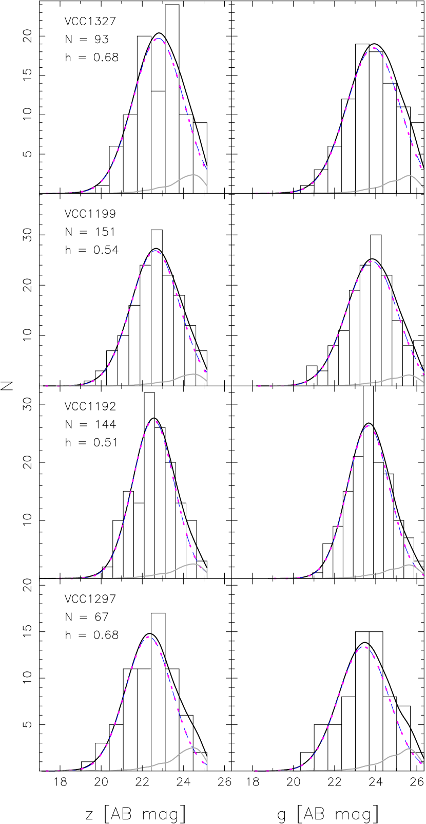
Figure 17.— Histograms and Gaussian fits for the GCLFs of GCs in the field of view of four companions of M87 (=VCC 1316) and M49 (=VCC 1226) that lie farther away than $6\,R_{e}$ from the companion galaxy, where $R_{e}$ is the effective radius of the companion and is determined as described in the text. For each field we present the $z$-band and $g$-band GCLFs side by side. The VCC name of the companion galaxy is indicated in the upper left corner of the left panel, where we also indicate the total number $N$ of sources with $p_{\rm GC}\geq 0.5$ and the bin-width $h$ used when constructing the histograms. In each panel we show the best fitting model (solid black curve), the intrinsic Gaussian component (dashed curve), the Gaussian component multiplied by the completeness fraction (dotted curve), and a kernel-density estimate of the expected contamination in the sample (solid gray curve). The solid black curve is the sum of the solid gray and dotted curves. Details of the fits are given in Table 6.

Figure 18.— (Left) GCLF turnover mass $M_{\rm TO}$ as a function of projected galactocentric distance $R_{\rm gc}$ in M49=VCC 1226 (top) and M87=VCC 1316 (bottom). Filled symbols refer to $z$-band measurements of $M_{\rm TO}$ while open symbols refer to $g$-band ones. (Right) Gaussian dispersion of logarithmic cluster masses, $\sigma_{M}$, as a function of projected galactocentric distance $R_{\rm gc}$ in M49=VCC1226 (top) and M87=VCC1316 (bottom). Filled symbols refer to $z$-band measurements while open symbols refer to $g$-band ones. In the M49 panels, the leftmost pairs of points refer to the GCLF parameters derived from the central ACS pointings in the main body of the galaxy; the next pair out correspond to the companion VCC 1192; and the rightmost pair correspond to the companion VCC 1199. In the M87 panels, the leftmost pairs of points refer to the GCLF parameters derived from the central ACS pointings in the main body of the galaxy; the next pair out correspond to the companion VCC 1297; and the rightmost pair correspond to the companion VCC 1327.

7. Discussion

We have found interesting trends in three mass scales of physical interest in connection with GC luminosity functions.

The GCLF turnover or peak mass takes a value of $M_{\rm TO}=(2.2\pm 0.4)\times 10^{5}\,M_{\odot}$ in most bright galaxies, but shows some downward scatter in dwarfs fainter than $M_{B,{\rm gal}}\gtrsim-18$. In M87 and M49, the data are consistent with a more or less constant $M_{\rm TO}$ to projected galactocentric radii of 20–35 kpc.

The higher-mass scale $M_{c}$ in an evolved Schechter function, which marks the onset of an exponential cut-off in the number of clusters per unit mass, grows steadily smaller in fainter galaxies. This drives a systematic narrowing of the dispersion in more traditional Gaussian fits to the GCLF, or equivalently a steepening of pure power-law fits to the mass function $dN/dM$ at cluster masses $M\gtrsim M_{\rm TO}$.

And the mass $\Delta$ in the evolved Schechter function, which controls the shape of the low-mass end of the GC mass distribution and is instrumental in setting $M_{\rm TO}$, varies by factors of a few—although not entirely monotonically—as a function of galaxy luminosity.

We now discuss these results in terms of their implications for GC formation and dynamical evolution. We begin by focusing on $\Delta$ in the evolved Schechter function, which, in the context of Fall & Zhang’s (2001) dynamical theory for the GCLF, is meant to measure the average amount of mass lost per globular cluster in a galaxy, over a Hubble time of evolution. We then move on to $M_{c}$ and $M_{\rm TO}$, asking specifically to what extent the observed variations in these high-mass characteristics of the GCLF might be caused by dynamical friction rather than initial conditions.

7.1. Evaporation and the Low-Mass Side of the GCLF

The defining feature of the evolved Schechter function in equation (7)—which we have found to fit the GC mass distributions of galaxies in the ACSVCS just as well as the traditional, but ad hoc, lognormal form—is the flat shape of $dN/dM$ in the limit of low masses. This asymptotic flatness always follows naturally from a time-independent rate of cluster mass loss, regardless of the assumed initial form of $dN/dM_{0}$ (Fall & Zhang 2001, and §3.2.2 above). The exact values of the average cumulative mass losses per GC for the galaxies in our sample are, however, more specific to the assumption that $dN/dM_{0}\propto M_{0}^{-2}\,\exp(-M_{0}/M_{c})$—a form chosen to match the observed mass functions of young massive clusters in local mergers and starbursts.

It is worth noting that, even though the average mass loss $\Delta$ in an evolved Schechter function is key to setting the GCLF turnover mass, $M_{\rm TO}$ does not vary as much or as systematically as $\Delta$ does in the ACSVCS sample (cf. Figures 15 and 16). This is because the value of the upper-mass cut-off $M_{c}$ also influences $M_{\rm TO}$ (see §3.2), and $M_{c}$ varies in such a way as to largely counteract the variation of $\Delta$, keeping $M_{\rm TO}$ more steady as a function of $M_{B,{\rm gal}}$.

Since $M_{\rm TO}$ is observed to be so nearly constant independently of any functional fitting—at least in large galaxies—this balance between variations in $\Delta$ and $M_{c}$ might be viewed simply as a necessary condition to make evolved Schechter functions match the data at all. But more interesting is that if the physical arguments behind the fitting function are close to correct, our results imply that the near-universality of the GCLF turnover in bright galaxies ($M_{B,{\rm gal}}\lesssim-18$) is in some sense a coincidence resulting from steeper initial $dN/dM$ (with lower $M_{c}$) in fainter systems being eroded by faster mass-loss rates (yielding larger $\Delta$).

As we discussed in §3.2, some amount of cluster mass loss may result from tidal shocks, but we expect that in general the largest part comes from two-body relaxation and evaporation, at a rate determined by the mean cluster density inside its half-mass radius: $\mu_{\rm ev}\propto\rho_{h}^{1/2}$. This basic dependence holds independently of any host galaxy properties, so if the cluster evaporation rate varies systematically as a function of $M_{B,{\rm gal}}$, it presumably reflects systematics in the typical $\rho_{h}$ of the cluster systems. Then, if GCs are tidally limited, such that their average densities are determined by the galaxy density inside their orbits (e.g., King 1962), variations in their characteristic $\rho_{h}$ should correspond in some way to variations in the host-galaxy densities. The easiest way to quantify any such connection is to assume a spherical, time-independent galaxy potential with a simple analytical form. Thus, in their models of the Milky Way GC system, Fall & Zhang (2001) relate the $\rho_{h}$ of individual clusters to their orbital pericenters $r_{p}$ in a logarithmic potential with a fixed circular speed, $V_{c}$, so that $\rho_{h}\propto\rho_{\rm gal}(r_{p})\propto V_{c}^{2}/r_{p}^{2}$. We address the validity of these particular (strong) assumptions about the host galaxy below; but for the moment we follow Fall & Zhang and most other authors (e.g., Vesperini 2000, 2001; Baumgardt & Makino 2003) in making them. What do our fitted $\Delta$ values for the ACSVCS galaxies then imply for the distribution of GC densities and pericenters in these systems?

The evaporation rate of a cluster with observable, projected half-mass radius $R_{h}$ depends on the density $\rho_{h}\equiv 3M/(8\pi R_{h}^{3})$ roughly as

$$\mu_{\rm ev}({\rm theo})\simeq 345\ M_{\odot}\,{\rm Gyr}^{-1}\ \left(\frac{\rho_{h}}{M_{\odot}\,{\rm pc}^{-3}}\right)^{1/2}\ ,$$ (21)

which again is independent of any assumptions on the host-galaxy potential. However, if $\rho_{h}$ is taken to be set by a well defined $r_{p}$ in a steady-state, singular isothermal sphere, then we also have (from eqs. [4] and [15] of Fall & Zhang 2001)

$$\mu_{\rm ev}({\rm theo}) \simeq 2.9\times 10^{4}\ M_{\odot}\,{\rm Gyr}^{-1}\,\left(r_{p}/{\rm kpc}\right)^{-1}\left(V_{c}/220\ {\rm km~{}s}^{-1}\right)$$ (22)

$$\quad\times\left[1-\ln\,(r_{p}/r_{c})\right]^{1/2}\ .$$

In the last term on the right-hand side, which is derived by Innanen, Harris, & Webbink (1983), $r_{c}$ is the radius of a circular orbit with the same energy as an arbitrary orbit with $r_{p}\leq r_{c}$.

Now, for the Milky Way, recall from §3.3 (eq. [14]), that we estimate

$$\Delta({\rm MW})=(2.5\pm 0.5)\times 10^{5}\,M_{\odot}$$ (23)

from our fit of an evolved Schechter function to the GCLF. For a GC age of 13 Gyr, this implies a mass-loss rate (averaged over the distribution of cluster $\rho_{h}$ or, given the assumptions behind eq. [22], over all cluster orbits) of

$$\langle\mu_{\rm ev}\rangle({\rm fit)}=\frac{\Delta({\rm MW})}{13\ {\rm Gyr}}=(1.9\pm 0.4)\times 10^{4}\,M_{\odot}\,{\rm Gyr}^{-1}\ .$$ (24)

Comparing equation (24) to equation (21) implies an average $\langle\rho_{h}\rangle\simeq(3000\pm 600)\,\,M_{\odot}\,{\rm pc}^{-3}$ for GCs in the Milky Way. This average falls towards the upper end of the range of cluster $\rho_{h}$ observed today, but it is within a factor of $\simeq\!2$–3 of the mean (e.g., see the data in Harris 1996). Equation (22) further suggests an average pericenter of $\langle r_{p}\rangle\approx 2$ kpc. This is roughly the same answer found by Fall & Zhang (2001; see their Figure 13), which shows that an evolved Schechter function is a reasonable analytical approximation to their full numerical theory. While such an $\langle r_{p}\rangle$ is slightly small—just as $\langle\rho_{h}\rangle$ is slightly high—compared to more direct pericenter estimates for Galactic globulars (cf. Innanen et al. 1983; van den Bergh 1995), it is again within the range of standard values.

It is not at all obvious a priori that average cluster densities and pericenters inferred strictly from fits to the Galactic GC mass function should agree to within factors of 2 or 3 with values estimated by independent methods. The fact that they do is an encouraging sign for the basic picture of evaporation-dominated GCLF evolution. Some residual corrections—downward in “predicted” $\langle\rho_{h}\rangle$ and up in $\langle r_{p}\rangle$—are evidently required, but at a level that plausibly could come from straightforward refinements in the various steps leading to equations (21) and (22). For example, there is some room for adjustment of the exact theoretical coefficients for the evaporation rate $\mu_{\rm ev}\propto M/t_{\rm rh}\propto\rho_{h}^{1/2}$ and the pericenter $r_{p}\propto\rho_{h}^{-1/2}$ (see, e.g., the discussions in Fall & Zhang 2001). In addition, we have neglected here any additional mass loss caused by tidal shocks, and we have adopted the idealization of a spherical and time-invariant Galactic potential.

To bring the ACSVCS data into this discussion, we focus on the basic pattern of variation in $\Delta$ as a function of galaxy luminosity, shown in the lower panel of Figure 16. First, $\Delta$ increases slightly from the brightest $M_{B,{\rm gal}}\simeq-21.5$ to the fainter $M_{B,{\rm gal}}\simeq-18$. The uncertainties and scatter in $\Delta$ are large, but the mean increase is perhaps a factor of $\approx\!2$–5. Then, at fainter $M_{B,{\rm gal}}\gtrsim-18$, $\Delta$ holds more constant or even decreases again, possibly by as much as a factor of $\approx\!2$–3 by the limiting $M_{B,{\rm gal}}\simeq-16$ of the survey.

If evaporation is responsible for these variations, then we should expect them to be mirrored in the behavior of the average GC half-mass radius as a function of galaxy luminosity: from equation (21), $\langle\mu_{\rm ev}\rangle\propto\langle\rho_{h}\rangle^{1/2}\propto\langle R_{h}\rangle^{-3/2}$, and by definition $\Delta\propto\langle\mu_{\rm ev}\rangle$ for coeval clusters. Globulars in Virgo are marginally resolved with the ACS, and Jordán et al. (2005) have fit PSF-convolved King (1966) models to estimate intrinsic $R_{h}$ values for individual sources (selected as described in §2 of Jordán et al. 2005) in most of the galaxies that we have dealt with here. The behavior of mean $\langle R_{h}\rangle$ versus $M_{B,{\rm gal}}$ is shown in Figure 5 of Jordán et al.

A detailed comparison of $\langle R_{h}\rangle$ and $\Delta$ is not straightforward, since these quantities were estimated separately for GC samples defined differently by Jordán et al. than in this paper. Nevertheless, it is interesting that $\langle R_{h}\rangle$ can be described as decreasing towards brighter galaxy luminosity in the range $-21.5\lesssim M_{B,{\rm gal}}\lesssim-18$, where $\Delta$ increases, and then turning around to increase somewhat at fainter $M_{B,{\rm gal}}\gtrsim-18$, where $\Delta$ decreases again. The changes in $\langle R_{h}\rangle$ are—as we would expect—smaller and less clear than those in $\Delta$, but it is just plausible that there is a net decrease of $\simeq\!35\%$ from $M_{B,{\rm gal}}=-21.5$ to $M_{B,{\rm gal}}=-18$ and a slightly larger increase from $M_{B,{\rm gal}}=-18$ to $M_{B,{\rm gal}}=-16$. This would be consistent with the shallowest trends able to fit $\Delta$ versus $M_{B,{\rm gal}}$ in Figure 16.

We cannot use equation (22) to relate $\Delta$ to typical GC pericenters and average galaxy densities on a case-by-case basis in the ACSVCS sample as in the Milky Way, since $V_{c}$ observations are not available for all systems. However, scaling relations can be used to some effect here. Large early-type galaxies with $M_{B,{\rm gal}}\lesssim-18$ generally obey $V_{c}=\sqrt{2}\sigma\propto L_{\rm gal}^{0.25}$ (e.g., Faber & Jackson 1976), $(M/L)_{\rm gal}\propto L_{\rm gal}^{0.2-0.3}$ at optical wavelengths (van der Marel 1991; Cappellari et al. 2006), and thus $R_{\rm eff}\propto L_{\rm gal}^{0.7-0.8}$ by the virial theorem (see also Haşegan et al. 2005). Average mass densities therefore increase towards lower $L_{\rm gal}$, such that equation (22) implies

$$\Delta\ \propto\ \left(R_{\rm eff}/\langle r_{p}\rangle\right)\,R_{\rm eff}^{-1}V_{c}\ \propto\ \left(R_{\rm eff}/\langle r_{p}\rangle\right)\,L_{\rm gal}^{-0.5\pm 0.05}$$ (25)

for bright galaxies. The situation is somewhat different for fainter $M_{B,{\rm gal}}\gtrsim-18$. For Coma Cluster galaxies in this regime, Matković & Guzmán (2005) find $V_{c}=\sqrt{2}\sigma\propto L_{\rm gal}^{0.5\pm 0.1}$, while the data in Graham & Guzmán (2003) suggest $R_{\rm eff}\propto L_{\rm gal}^{0.1-0.2}$. If these systems are representative of those in Virgo, then their average densities decrease towards lower $L_{\rm gal}$, and equation (22) leads to

$$\Delta\ \propto\ \left(R_{\rm eff}/\langle r_{p}\rangle\right)\,L_{\rm gal}^{0.35\pm 0.1}$$ (26)

for faint dwarfs.

The major unknown in equations (25) and (26) is the ratio of galaxy $R_{\rm eff}$ to GC $\langle r_{p}\rangle$, and how it might or might not vary systematically as a function of galaxy luminosity. If the ratio is constant for all systems, then the dotted lines drawn in the lower panel of Figure 16 show the expected variation of the mass loss $\Delta$ versus $M_{B,{\rm gal}}$. These lines are normalized to make $\Delta=2.5\times 10^{5}\,M_{\odot}$ at $M_{B,{\rm gal}}=-21$ and to make the bright- and faint-galaxy scalings meet at $M_{B,{\rm gal}}=-18$. The net increase of $L_{\rm gal}^{-0.5}$ from $M_{B,{\rm gal}}=-21.5$ to $M_{B,{\rm gal}}=-18$ is a factor of about 5, while the decrease of $L_{\rm gal}^{0.35}$ from $M_{B,{\rm gal}}=-18$ to $M_{B,{\rm gal}}=-16$ is a factor of approximately 2.

These changes may be somewhat greater than suggested by the actual fitted estimates of $\Delta$. Moreover, an increase of $\Delta$ by a factor of 5 between $M_{B,{\rm gal}}=-21.5$ and $M_{B,{\rm gal}}=-18$ would imply a decrease in $\langle R_{h}\rangle$ by a factor of $5^{2/3}\approx 3$, which is larger than the measurements of Jordán et al. (2005) support. However, this is clearly not an order-of-magnitude problem. It could easily be alleviated if the galaxy total mass distributions are not isothermal spheres, or if $R_{\rm eff}/\langle r_{p}\rangle$ depends even weakly on galaxy luminosity, or if uncertainties and scatter in the galaxy scalings result in small deviations from the nominal exponents on $L_{\rm gal}$ in equations (25) and (26). Tidal shocks may also contribute differently to the net $\Delta$ in different galaxies, a complication that we have entirely ignored. Again, then, it is encouraging that these crude relations come as close as they do to explaining the systematics in a cluster mass-loss parameter inferred only from the GCLF—accounting in particular for the change in dependence of $\Delta$ on galaxy luminosity around $M_{B,{\rm gal}}\simeq-18$.

Obviously, more rigorous and detailed analyses of individual galaxies are required to really make (or break) the case in general that the overall form of an evolved Schechter function for the GC mass function, and the parameter $\Delta$ especially, can be interpreted physically and self-consistently as the result of evolution from an initial GC $dN/dM_{0}\propto M_{0}^{-2}$ with individual cluster mass-loss rates that are constant in time. From our discussion here, it does seem that this “literal” view of the simple fits to the Milky Way and ACSVCS GCLFs is at least broadly compatible with observations of the cluster densities or radii in these galaxies and with the trends in $\Delta$ vs. $L_{\rm gal}$, if evaporation is the main disruptive process for clusters as massive as $M_{\rm TO}\sim 2\times 10^{5}\,M_{\odot}$.

Difficulties do arise, however, when considering the additional constraint that the GCLF is invariant over wide ranges of galactocentric radius and GC density in the Milky Way and other large galaxies. As described above, application of equation (22) to the global Galactic GCLF ultimately implies an average GC pericenter of $\langle r_{p}\rangle\simeq 2$ kpc, corresponding to about half the effective radius of the bulge. Similarly, our normalization of equation (25) in Figure 16 implies $\langle r_{p}\rangle<0.5\,R_{\rm eff}$ for the brightest early-type galaxies in Virgo. But observationally, the GCLF turnover $M_{\rm TO}$ (and thus $\Delta$) has the same, global value for clusters currently found out to at least 10–15 effective radii in the Milky Way (e.g., Harris 2001) and at least $\simeq 4\,R_{\rm eff}$ in M87 and M49 (§6.3). This can only be consistent with evaporation-dominated depletion of an intially steep GC $dN/dM_{0}\propto M_{0}^{-2}$ at low masses, and with the additional assumption that the mass loss $\Delta\propto r_{p}^{-1}$, if cluster orbits are systematically much more elongated at larger galactocentric radius in all these systems.

In fact, for the Milky Way and M87 respectively, Fall & Zhang (2001) and Vesperini et al. (2003) have shown that following this chain of logic leads to the conclusion that globulars should initially have been on predominantly radial orbits outside about one effective radius in each galaxy. On the other hand, the present GC velocity distributions in the Galaxy, in M87, and in M49 are all essentially isotropic—implying orbits with typical axis ratios of only $r_{a}/r_{p}\simeq 3$—out to the same spatial scales of several $R_{\rm eff}$, over which the observed GCLF is invariant (see, e.g., Dinescu, Girard, & van Altena 1999; Côté et al. 2001, 2003). Fall & Zhang suggest that this difference between (presumed) initial and (observed) present orbital properties might be explained by preferential depletion of GCs on the most radial orbits. But while the idea remains to be tested in detail for the Milky Way, Vesperini et al. (2003) show that—again if the galaxy potential is spherical and time-independent—it does not suffice to account quantitatively for the combined GCLF and kinematics data in M87.

Related to this is the average density, $\langle\rho_{h}\rangle\simeq 3000\ M_{\odot}\,{\rm pc}^{-2}$, implied by the more general equation (21) and the required total $\Delta$ for Galactic globulars. A similar $\langle\rho_{h}\rangle$ is also suggested for GCs in the brightest Virgo galaxies by the $\Delta$ values in Figure 16. As we mentioned above, such densities are observed for real clusters; but there is a broad distribution of $\rho_{h}$, with an average slightly lower than $3000\ M_{\odot}\,{\rm pc}^{-2}$ and a long tail to much smaller values of $<\!100\ M_{\odot}\,{\rm pc}^{-2}$. More generally, the GCs in most large galaxies have half-mass radii that are largely uncorrelated with cluster mass (e.g., van den Bergh, Morbey, & Pazder 1991; Jordán et al. 2005, and references therein), so that $\rho_{h}$ apparently always ranges over more than two orders of magnitude. When $\rho_{h}<100\ M_{\odot}\,{\rm pc}^{-2}$, the total evaporative mass loss per cluster over 13 Gyr is $<5\times 10^{4}\,M_{\odot}$, well below the typical average $\Delta$ and global $M_{\rm TO}$ for entire GC systems. In the Milky Way at least, the large majority of such low-density GCs are found at Galactocentric distances $r_{\rm gc}\gtrsim 10$ kpc, so in a sense the problem is bound up with the weak radial variation of the GCLF.

These points are important, and they need to be resolved, but they should not be taken as disproof of the idea that long-term dynamical evolution alone might explain the difference between the mass functions of old GCs and young massive clusters. Ultimately, the near-flatness of $dN/dM$ at low masses, which is clearly seen in the Milky Way and is entirely consistent with all of our Virgo GCLFs, only demands that cluster masses decrease linearly in time if the dynamical-evolution hypothesis is correct at all (see Fall & Zhang 2001, and §3.2 above). It is not absolutely necessary that evaporation account for the full mass-loss rate of every cluster, even though our discussion here has focused on exploring this possibility (and shown that it does come remarkably close, to within factors of 2–3 for the most part). For example, globulars in the extreme low-density tails of $\rho_{h}$ distributions, mentioned just above, might be much more strongly—and differently—affected by tidal shocks than any previous GCLF calculations have allowed. Such shock-dominated evolution could still lead to a constant mass-loss rate of its own (see Dehnen et al. 2004, and §3.2.2 above), which would add directly to $\mu_{\rm ev}$ without otherwise changing any of the main arguments here.

In more specific terms, the radial invariance of the GCLF might ultimately be explained by modifying a single ancillary assumption in the current dynamical-evolution models rather than discarding the idea altogether. It is the notion of spherical and steady-state galaxy potentials that prompts Fall & Zhang (2001), Vesperini et al. (2003), and almost all other authors to use equations (21) and (22) to tie cluster densities to orbital pericenters in these analyses. But, as Fall & Zhang themselves point out, this is of course an extreme simplification for galaxies that grow through hierarchical merging.

Fall & Zhang suggest, for example, that a major merger could obviate the need for extremely radial orbits to distribute clusters with high mean densities, fixed at small and well defined pericenters, over large volumes in a galaxy. Instead, a merger may efficiently mix two globular cluster systems spatially and isotropize their velocity distribution. This could then work to weaken any radial gradients in the mass loss $\Delta$ and the GCLF turnover mass, which might have resulted from realistic orbital distributions and $\mu_{\rm ev}(r_{p})$ dependence like equation (22) in the progenitor galaxies.

In addition to this, multiple minor mergers—which are perhaps more relevant than major mergers for a galaxy like our own—should steadily bring in globulars formed with densities and evaporation rates unrelated, at least initially, to their new orbits in the main galaxy, making the use of equation (22) less than straightforward. In fact, any use of it at all could be questionable in this case, since all clusters would constantly be sampling new pericenters in an evolving potential. Again, then, weak spatial variations in $\Delta$ and $M_{\rm TO}$ need not imply highly radial GC orbits. Prieto & Gnedin (2006) have recently simulated the evolution of the GCLF during the hierarchical growth of a Milky Way-sized galaxy. Starting from an initial cluster mass function $dN/dM_{0}\propto M_{0}^{-2}$, which is re-shaped primarily by evaporation—but abandoning equation (22) and instead adopting evaporation rates from GC densities fixed independently of their orbits—they find that it is possible (even without a recent major merger) to produce a final GC system with an isotropic velocity distribution and a radially invariant GCLF similar to the observed Galactic distribution.

A caveat is that the hierarchical-growth simulations most favored by Prieto & Gnedin (2006) are ones in which they assume that all globular clusters have a common mean density inside $R_{h}$ (just one that is not set by any orbital pericenter). This is still incompatible with the wide range of $\rho_{h}$ observed for the GCs in many galaxies, and it is furthermore not obvious how the cumulative mass loss $\Delta\propto\langle\rho_{h}\rangle^{1/2}$ should then vary as a function of galaxy luminosity. On the other hand, Prieto & Gnedin have also run some models allowing for an initial spread of GC densities followed by evaporation at constant $\rho_{h}$. This is at least more reminiscent of real $\rho_{h}$ distributions, and it still produces a GCLF that is not too drastically different from the Galactic one. Clearly, more work is required to clarify the dynamical evolution of initial power-law GC mass functions in time-dependent galaxy potentials, with the totality of relevant observational constraints taken into account: a flat $dN/dM$ at low masses; a weak or absent correlation between GC radii and masses; radially invariant GCLFs; currently isotropic velocity distributions; and mass losses $\Delta$ that vary with galaxy luminosity as in Figure 16.

Should all efforts along these lines fail to explain the combined data, the only option left would seem to be that a peak in the GCLF was established much earlier, by processes more related to cluster formation. One possible scenario has been proposed by Vesperini & Zepf (2003). They suggest that low-mass globulars were initially less concentrated (with a larger ratio of half-mass to tidal radius) than high-mass clusters. The inevitable expansion of all clusters following mass loss driven by stellar evolution would then cause many low-mass clusters preferentially to overflow their tidal radii, leading ultimately to fast disruption times of a few hundred Myr or less (Chernoff & Weinberg 1990). This may turn an initial power-law $dN/dM_{0}$ at low masses into a roughly flat-topped or even lognormal distribution, with $M_{\rm TO}$ near its current value, very early on. Weaker long-term evaporation (i.e., lower cluster densities or larger and more variable pericenters) could then suffice to explain the residual difference between the initial, steep mass function and the final, observed one, even in a static galaxy potential.

Observations of the young massive clusters in the Antennae galaxies already imply that early disruption is independent of cluster mass, at least for clusters more massive than several $10^{4}\,M_{\odot}$ and younger than $\simeq\!10^{8}$ yr (Zhang & Fall 1999; Fall et al. 2005). Thus, if the disruption mechanism of Vesperini & Zepf (2003) is to work, the mass-selective aspect of it apparently must be restricted to timescales of $10^{8}$–$10^{9}$ yr or so. In any case, the success of this or any similar picture further relies on an appropriately tuned mass dependence in some key GC property being built into cluster systems essentially as an initial condition; but this still requires explanation in itself.

7.2. Dynamical Friction and the High-Mass Side of the GCLF

At GC mass scales $M\gtrsim\Delta$, dynamical friction can in some cases become more important than evaporation or shocks as a cluster destruction mechanism. A point mass $M$ originally on a circular orbit of radius $r$ in a galaxy with a total-mass distribution following a singular isothermal sphere will spiral in to the galaxy center within a time (Binney & Tremaine 1987)

$$\tau_{\rm df}\simeq\frac{5.9\ {\rm Gyr}}{(\ln\Lambda)/10}\left(\frac{r}{{\rm kpc}}\right)^{2}\left(\frac{V_{c}}{220\ {\rm km\ s}^{-1}}\right)\left(\frac{10^{6}\,M_{\odot}}{M}\right)\ ,$$ (27)

where $V_{c}$ is the galaxy’s circular speed and $\ln\Lambda\sim 10$ is the usual Coulomb logarithm.

It is clear from equation (27) that dynamical friction cannot be a major factor in deciding the evolution of all but the very most massive tip of the GCLF in $\sim\!L_{*}$ and brighter galaxies with $V_{c}\gtrsim 200$ km s^-1. However, the scaling $\tau_{\rm df}\propto V_{c}$ implies that the relevance of dynamical friction can increase significantly for lower luminosity galaxies (e.g., Hernandéz & Gilmore 1998; Lotz et al. 2001). It is then reasonable to ask whether a stronger depletion of massive GCs in dwarf galaxies might be able to explain the systematic decrease of $M_{c}$ versus $M_{B,{\rm gal}}$ in our fits of evolved Schechter functions for these systems, and possibly even the slight decrease in average $M_{\rm TO}$ towards the faintest $M_{B,{\rm gal}}$.

Figure 19.— A simple model for the effects of dynamical friction on the GC mass function, illustrated in terms of the distribution $dN/d\,\log\,M$, which is directly proportional to the GCLF. The solid curve shows this version of an evolved Schechter function with $M_{c}=3.0\times 10^{6}\,M_{\odot}$ and $\Delta=2.6\times 10^{5}\,M_{\odot}$ (hence $M_{\rm TO}=2.2\times 10^{5}\,M_{\odot}$), appropriate for a giant elliptical. This is assumed to be the mass function on which dynamical friction operates. The monotonically decreasing dotted curve shows the function $S(M,t=13\ {\rm Gyr})$ (eq. [30]), calculated for a galaxy with $M_{B,{\rm gal}}=-21.75$ as described in the text. The dotted bell-shaped curve is the product of this $S$ times the solid curve; it illustrates the cumulative effect of dynamical friction on the GCLF in very massive galaxies. The monotonically decreasing dashed curve shows the function $S(M,t=13\ {\rm Gyr})$ as calculated for a galaxy with $M_{B,{\rm gal}}=-15.75$. The dashed bell-shaped curve is the product of this $S$ times the solid curve, illustrating the net effect of dynamical friction on the GCLF in very faint galaxies. The arrows indicate the position of the final turnover mass for each of the resulting mass functions. There is a slight decrease in $M_{\rm TO}$ for the low-luminosity galaxy as a consequence of dynamical friction, but not enough to account fully for the observed behavior in Fig. 15 or Fig. 12.

We do not attempt here to find a definitive answer to this question, but only an indication of the ability of dynamical friction to produce the observed trends. One particular subtlety is that the expression for $\tau_{\rm df}$ in equation (27) does not allow for clusters to evaporate. But a steadily decreasing cluster mass will lead to a longer total dynamical-friction timescale. We deal with this complication in the simplest way possible: the timescale $\tau_{\rm df}$ for a cluster with initial mass $M_{0}$ and present mass $M=(M_{0}-\Delta)$ is approximated by evaluating equation (27) at the average mass, $(M+\Delta/2)$.

Let us denote by $\widehat{\Psi}(M,t)$ the GC mass function that would be obtained after a time $t$ of GC evolution in the absence of any dynamical friction. The effects of dynamical friction are easily accounted for by subtracting from $\widehat{\Psi}$ all clusters with instantaneous masses $M$ such that

$$(M+\Delta/2)>M_{\rm min}(r,t)\ ,$$ (28)

where $M_{\rm min}$ follows from equation (27) by setting $\tau_{\rm df}<t$:

$$M_{\rm min}(r,t)\simeq\frac{4.5\times 10^{5}\,M_{\odot}}{(\ln\Lambda)/10}\left(\frac{13\ {\rm Gyr}}{t}\right)\left(\frac{r}{{\rm kpc}}\right)^{2}\left(\frac{V_{c}}{220\,{\rm km\ s}^{-1}}\right)\ .$$ (29)

The net, “global” GC mass function (averaged over all GC orbits, or galactocentric radii) at any time $t$ is thus $dN/dM=S(M,t)\times\widehat{\Psi}(M,t)$ where

$$S(M,t)=\frac{\int_{0}^{\infty}\rho_{\rm GC}(r)\,H[M_{\rm min}(r,t)-(M+\Delta/2)]\,4\pi r^{2}\,dr}{\int_{0}^{\infty}\rho_{\rm GC}(r)\,4\pi r^{2}\,dr}\ .$$ (30)

Here $\rho_{\rm GC}(r)$ is the space density of GCs (assumed to be independent of cluster mass) and $H$ is the Heaviside step function: $H(x)\equiv 1$ for $x>0$ and $H(x)\equiv 0$ for $x<0$.

This raises further points to be dealt with in more careful calculations along these lines. First, dynamical friction will clearly affect also the spatial distribution of GCs, so that $\rho_{\rm GC}(r)$ will have a dependence on time, which we ignore. Second, the effects of dynamical friction could introduce some dependence on galactocentric position into the GC mass function, which in a complete treatment would be contrasted with observational limits on any such variations. Third, changing the assumed galaxy potential could significantly affect the derived $\tau_{\rm df}$ (e.g., Hernandez & Gilmore 1998; Read et al. 2006), as could relaxing the unrealistic assumption of strictly circular orbits (e.g., Pesce, Capuzzo-Dolcetta, & Vietri 1992; van den Bosch et al. 1999). Finally, we do not take into account the fact that the ACS has a fixed field of view, and thus we are not always observing truly globally averaged GCLFs—although this point is relevant mainly for the most massive galaxies, where the effects of dynamical friction are expected to be negligible in any case.

These issues notwithstanding, we proceed to estimate the effects of dynamical friction by evaluating $S(M,t)$ as written in equation (30). We assume that the “friction-free” $\widehat{\Psi}(M,t)$ at the present day is well described by the GCLF of bright ellipticals, where dynamical friction is negligible, and is therefore given by equation (7) with $\Delta=2.6\times 10^{5}M_{\odot}$ and $M_{c}=3\times 10^{6}M_{\odot}$ (see Figure 16 and Table 3). To obtain the final $dN/dM$ including dynamical friction, we then multiply this by the function $S(M,t\equiv 13\,{\rm Gyr})$. In doing so, we always take the slowly varying Coulomb logarithm in equation (29) to be $\ln\Lambda=10$.

We assume that for giant galaxies with $M_{B}<-18$ we have $V_{c}\propto\sigma\propto L_{\rm gal}^{0.25}$ (Faber & Jackson 1976), with a zeropoint chosen to give $V_{c}=484$ km s^-1 at $M_{B}=-21.75$, based on the velocity dispersion of M87 (Bender, Saglia & Gerhard 1994). We impose a change in this scaling at $M_{B}>-18$, so that dwarfs follow $V_{c}\propto\sigma\propto L_{\rm gal}^{0.5\pm 0.1}$ (Matković & Guzmán 2005; cf. §7.1 above). We can then find $M_{\rm min}(r,t)$ from equation (29) for any GC in any galaxy.

To specify the spatial distribution of GCs and calculate $S(M,t=13\ {\rm Gyr})$, we estimate the galaxy’s effective radius $R_{\rm eff}$ using the data from Ferrarese et al. (2006a); then we assume that the effective radius of the GC system is just twice $R_{\rm eff}$ (Peng et al. 2006, in preparation). Finally, we assume that $\rho_{\rm GC}(r)$ is given by the density profile of Prugniel & Simien (1997; see also Terzić & Graham 2005), which is an analytical approximation to the deprojection of a Sersic profile ($R^{1/n}$ law), and we let the Sersic index $n$ be determined by $M_{B,{\rm gal}}$ as per equation (25) of Ferrarese et al. (2006a).

The results of the calculations for two representative galaxy magnitudes, $M_{B,{\rm gal}}=-21.75$ and $M_{B,{\rm gal}}=-15.75$, are illustrated in Figure 19. The figure shows both $S(M,t=13\ {\rm Gyr})$ (the monotonically decreasing curves) and the function $dN/d\log M$ (proportional to the GCLF and given by the peaked curves) that follows from dynamical friction acting on the assumed evolved Schechter function. The resulting turnover mass scales are indicated with arrows, which show that the stronger dynamical friction in the fainter galaxy leads to a slightly lower turnover mass scale.

We show the behavior of $M_{\rm TO}$ as a function of $M_{B,{\rm gal}}$ in general, in the upper panel of Figure 20 (circles connected by a solid line) and contrast it with the observed variation in our binned-galaxy GC samples (Figure 15). The predicted $M_{\rm TO}$ varies quite slowly with $M_{B,{\rm gal}}$, but it ultimately decreases by $\sim 10\%$ from our assumed $2.2\times 10^{5}\,M_{\odot}$ in the brightest galaxies. This is comparable to the observed decrease of $\approx\!30\%$ in $M_{\rm TO}$. Thus, dynamical friction may be responsible for some part of the the slow change in GCLF turnover mass with galaxy magnitude.

Figure 20.— (Upper panel) GCLF turnover mass $M_{{\rm TO},z}$, inferred from evolved Schechter fits to $z$-band data for the binned-galaxy GC samples, versus $M_{B,{\rm gal}}$ (data are the same as the circles in Fig. 15). The open symbols connected by a solid line are the predicted change in $M_{\rm TO}$ due to the increasing efficiency of dynamical friction in fainter galaxies; see text. Dynamical friction might account for part of the observed trend, but probably not all of it. (Lower panel) Evolved Schechter function cut-off mass $M_{c,z}$ versus $M_{B,{\rm gal}}$ for binned-galaxy $z$-band samples. The open symbols connected by a solid line are again our predictions for the change in $M_{c}$ due to stronger dynamical friction in smaller galaxies. Dynamical friction is not able to explain the observed behavior of $M_{c}$ as a function of galaxy luminosity.

In the lower panel of Figure 20 we show (again, as open circles connected by a solid line) the $M_{c}$ values inferred by fitting evolved Schechter functions to our model GC mass functions after calculating the effects of dynamical friction. Evidently, we can expect dynamical friction to cause perhaps a $\sim\!30\%$–40% decrease in the value of $M_{c}$ from the brightest to the faintest galaxies; but this is altogether too little to account for the factor of $\simeq\!6$–7 decrease we actually observe. Similarly, if we fit power laws to our dynamical-friction mass functions in the range $3\times 10^{5}\,M_{\odot}\leq M\leq 2\times 10^{6}\,M_{\odot}$, we obtain rather constant powers $\beta\simeq 1.7$–1.8 for galaxy magnitudes $-21.75<M_{B,{\rm gal}}<-15.75$, which is far from being able to explain the observational situation in Figure 10 above. We conclude that dynamical friction cannot account for more than a small fraction of the observed steepening of the globular cluster mass function above the GCLF turnover.

These results are essentially in agreement with those of Vesperini (2000), who models the effects of evaporation and dynamical friction on the GCLF, and predicts only slight decreases in the mean $\langle\log\,M\rangle$ and the Gaussian dispersion $\sigma_{M}$ as galaxy luminosity decreases (see his Figure 6), at levels much smaller than those seen in our data (e.g., Figure 14). Thus, although we have emphasized the highly simplified nature of our calculations, it nevertheless appears that galaxy-to-galaxy systematics in the cluster formation processes, rather than dynamical evolution, must be largely responsible for the observed variation in the detailed form of the GCLF at high masses.

7.2.1 Initial Conditions

It seems inevitable from the discussion above that the observed steepening or narrowing of the GCLF above the turnover point $M_{\rm TO}\sim 2\times 10^{5}\,M_{\odot}$ in fainter galaxies—whether this is expressed in terms of smaller Schechter-function mass scales $M_{c}$ or steeper power-law indices $\beta$ or narrower Gaussian dispersions $\sigma_{M}$—must reflect non-universal initial conditions in the cluster mass distribution, and therefore some fundamental aspect of the star-formation process.

Observationally, it is known that the luminosity of the brightest young star cluster in a star-forming galaxy scales with the global star formation rate (Billet, Hunter & Elmegreen 2002; Larsen 2002). There has been some discussion as to whether this is just a size-of-sample effect (if more clusters are formed, it is statistically more likely to achieve higher masses by random sampling of an underlying mass distribution that might still be universal) or indicative of a real, physical limit to the initial cluster mass function (Larsen 2002; Weidner, Kroupa & Larsen 2004).

Gieles et al. (2006a, b) argue that there is a physical upper limit, $M_{\rm max}$, to cluster masses in each of NGC 6946, M51, and the Antennae galaxies (though see Whitmore, Chandar & Fall 2006 for a differing view). The number of clusters found with $M>M_{\rm max}$ falls rapidly to zero in all three cases, but the value of the upper limit is found by Gieles et al. to vary between the galaxies, from $M_{\rm max}\simeq 4$–$10\times 10^{5}\,M_{\odot}$. Qualitatively, a parameter like $M_{\rm max}$ can be identified with $M_{c}$ in a Schechter-function description of (initial) GC mass functions. Quantitatively, the range of $M_{\rm max}$ claimed by Gieles et al. for their young systems is very similar indeed to our fitted $M_{c}$ values for the old GCs in early-type Virgo galaxies (see Figure 16).

It will be interesting to explore this possible connection between globulars and young massive clusters in more detail. Possibly one route to take is suggested by the theory of the GCLF developed by Harris & Pudritz (1994), in which a distribution of cluster masses is built up by collisions between gaseous protoclusters. McLaughlin & Pudritz (1996) suggest that the total time required to produce very high-mass clusters may be longer for galaxies in lower-density environments, and this could perhaps be related to our finding of a cut-off at lower $M_{c}$ (in our current notation) for the initial GC mass functions at fainter $M_{B,{\rm gal}}$. If these types of ideas can be generalized, then both our GCLF observations and the possible existence of an upper mass “limit” in young cluster systems could be reflecting a systematic variation in gas-dynamical timescales as a function of galaxy mass and/or density.

In any case, the fact that dynamical friction is unable to account for the steepening of an initially universal mass function as the mass of the host galaxy decreases, combined with the possible existence in young, relatively unevolved cluster systems of a mass scale similar to $M_{c}$ in our old GC systems, leads us to favor the view that a significant part of the observed morphology at the highest-mass ends of GCLFs is due to systematics in the initial distributions. The precise extent to which this part of the initial mass function is still reflected in the present-day one is still something of an open question, the answer to which will be a crucial ingredient in our understanding of GC formation and evolution. A detailed understanding of the “microscopic” star-formation processes on rather short timescales in very young clusters could well be key to making much further progress in this direction.

8. Summary and Conclusions

We have presented the GCLFs of 89 early-type galaxies in the Virgo cluster and determined maximum-likelihood estimates for model parameters using fits of Gaussians and a simple “evolved Schechter function” described in §3.2. The latter reflects the effects of GC disruption (at a constant rate and presumably due mostly to two-body relaxation and evaporation) on an initial cluster mass distribution that followed a Schechter function with a fixed power-law index of $-2$ at low masses. The evolved mass function tends to a flat shape at low $M$ and is an accurate analytical approximation to the numerical distributions produced in the theory of Fall & Zhang (2001). We have tested the robustness of our results by simulations, by the construction of GCLFs for galaxies binned together to contain a minimum number of clusters, and by using alternate schemes to select GC candidates from catalogues of observed sources. Our main results and conclusions are the following:

1. We find a remarkably regular decrease of the dispersion of the GCLF as the luminosity of the host galaxy decreases (§6 and Jordán et al. 2006). Quantitatively, the maximum-likelihood estimates of the dispersion $\sigma$ of Gaussian fits to the $z$- and $g$-band data are well described by the linear relations presented in equations (17) and (18). The dispersions for the GCLFs of the Milky Way and M31 fall in the midst of our new data and thus the correlation of $\sigma$ with $M_{B,{\rm gal}}$ would appear to be more fundamental than the older view, that GCLF widths depend on galaxy Hubble type.

   This trend reflects a systematic steepening of the GC mass function for massive clusters in particular ($M\gtrsim 3\times 10^{5}M_{\odot}$, above the peak of the GCLF) as the host galaxy luminosity decreases. When fitting power-law mass functions to this upper cluster mass regime, the power-law exponents in a model of the form $dN/dM\propto M^{-\beta}$ increase from $\beta\lesssim 2$ to $\beta\gtrsim 3$ over the range of galaxy masses in our sample. This steepening is in turn equivalent to a systematic decrease of the cut-off mass $M_{c}$ in evolved-Schechter function fits to the GCLFs, from $M_{c}\simeq 2$–$3\times 10^{6}\,M_{\odot}$ in the brightest galaxies to $M_{c}\simeq\,3$–$4\times 10^{5}\,M_{\odot}$ in the faintest systems.

2. The GCLF turnover mass $M_{\rm TO}$ is slightly smaller in dwarf systems ($M_{B}\gtrsim-18$), relative to the same quantity in more massive galaxies. In the latter we have $M_{\rm TO}=(2.2\pm 0.4)\times 10^{5}M_{\odot}$, decreasing to $M_{\rm TO}\simeq 1.6$–$1.7\times 10^{5}M_{\odot}$ on average for the faintest galaxies in our sample—although individual dwarfs scatter between $1\times 10^{5}\,M_{\odot}\lesssim M_{\rm TO}\lesssim 2\times 10^{5}\,M_{\odot}$ (§6). We show that this might be at least partly accounted for by the effects of dynamical friction if all other processes shaping the mass function were to lead to an invariant $M_{\rm TO}$ (§7.2).

3. We explored radial variations of the GCLF over baselines of $20-35$ kpc in M87 (VCC 1316) and M49 (VCC 1226) by studying GCs in the fields of dwarf galaxies close in projection to these giant ellipticals (§6.3). We find no evidence for a variation of the turnover mass $M_{\rm TO}$ with galactocentric distance in either galaxy, consistent with previous studies of M87 in particular. This reinforces the importance of the radial invariance of GCLFs as a constraint on models of GCLF formation and dynamical evolution.

4. Our success in fitting evolved Schechter functions to our data (§5.2) means that the GC mass functions in early-type Virgo galaxies are consistent with a universally flat shape, $dN/dM\sim{\rm constant}$, in the limit of low masses—as is also found in the Milky Way (§3.3 and Fall & Zhang 2001). If this feature is caused by dynamical evolution from a much steeper initial distribution, it requires that cluster masses decrease linearly in time. This can plausibly be expected if evaporation dominates the cluster evolution, although tidal shocks may also lead to similar behavior.

5. Fits of the evolved Schechter function imply that a narrow range of average mass losses per GC—$\Delta\approx(2$–$10)\times 10^{5}M_{\odot}$ at the outside—is required in all galaxies to account for our observed GCLFs. Such a range of $\Delta$ across a factor of $\approx\!400$ in galaxy luminosity is in rough agreement with observed (small) variations in the mean half-mass radii of GCs in the ACSVCS galaxies (Jordán et al. 2005), and with simple scalings of evaporation rate as a function of host-galaxy luminosity (§7.1). However, more work is required to reconcile fully the main idea—that long-term dynamical evolution alone transformed initial Schechter cluster mass functions into the presently observed distributions—with the weak radial variation of GCLFs inside large galaxies and with observations of the orbital distributions and range of mean cluster densities in the same systems.

6. The clear decrease of the GC cut-off mass $M_{c}$ with galaxy luminosity in evolved-Schechter function descriptions of the GCLF (§5.2) is too pronounced to be explained by dynamical friction operating on a universal $dN/dM$ with an initially constant $M_{c}$ in all galaxies (§7.2). It most likely reflects systematic variations at the high-mass end of the initial GC mass function.

The present-day mass functions of GCs were likely shaped by a variety of processes acting on different timescales, including systematic variations in the initial (proto-)cluster mass function at the high-mass end; long-term dynamical erosion by evaporation, tidal shocks, and dynamical friction; and global relaxation effects in time-varying galaxy potentials (hierarchical merging). It is further possible, though not yet entirely clear, that mass-selective early dissolution of clusters due to stellar evolution may have played some role in defining the observed mass distributions. Future attempts to understand the whole of the GCLF will clearly have to consider all of these processes, and their inevitable interplay, in quite some detail. Such comprehensive modeling will also have to acknowledge the increasingly complex and stringent empirical constraints that follow from combining direct GCLF observations with other GC systematics—such as their structural correlations, and the dynamics of cluster systems—for which data are continually accumulating and improving in quality.

Table 1Luminosity Function Histograms for GCs and Expected Contaminants

	Sample with $p_{\rm GC}\geq 0.5$											Sample with $m_{z}<25.15$ or $m_{g}<26.35$, and $R_{h}<0\farcs 064$
VCC	$m_{z}$	$h_{z}$	$N_{z,\rm tot}$	$N_{z,\rm cont}$	$f_{z}$	$m_{g}$	$h_{g}$	$N_{g,\rm tot}$	$N_{g,\rm cont}$	$f_{g}$		$m_{z}$	$h_{z}$	$N_{z,\rm tot}$	$N_{z,\rm cont}$	$f_{z}$	$m_{g}$	$h_{g}$	$N_{g,\rm tot}$	$N_{g,\rm cont}$	$f_{g}$
(1)	(2)	(3)	(4)	(5)	(6)	(7)	(8)	(9)	(10)	(11)		(12)	(13)	(14)	(15)	(16)	(17)	(18)	(19)	(20)	(21)
1226	18.0	0.4	0	0.0	1.00	19.2	0.4	0	0.0	1.00		18.0	0.4	0	0.1	1.00	19.2	0.4	0	0.1	1.00
1226	18.4	0.4	0	0.1	1.00	19.6	0.4	0	0.1	1.00		18.4	0.4	0	0.2	1.00	19.6	0.4	0	0.2	1.00
1226	18.8	0.4	2	0.0	1.00	20.0	0.4	1	0.1	1.00		18.8	0.4	0	0.2	1.00	20.0	0.4	0	0.2	1.00
1226	19.2	0.4	5	0.2	1.00	20.4	0.4	3	0.1	1.00		19.2	0.4	5	0.2	1.00	20.4	0.4	2	0.1	1.00
1226	19.6	0.4	4	0.3	1.00	20.8	0.4	8	0.4	1.00		19.6	0.4	4	0.3	1.00	20.8	0.4	8	0.5	1.00
1226	20.0	0.4	12	0.2	1.00	21.2	0.4	11	0.3	1.00		20.0	0.4	12	0.2	1.00	21.2	0.4	10	0.4	1.00
1226	20.4	0.4	25	0.4	1.00	21.6	0.4	24	0.2	1.00		20.4	0.4	24	0.5	1.00	21.6	0.4	23	0.4	1.00
1226	20.8	0.4	32	0.2	1.00	22.0	0.4	33	0.3	1.00		20.8	0.4	31	0.4	1.00	22.0	0.4	33	0.3	1.00
1226	21.2	0.4	57	0.4	1.00	22.4	0.4	59	0.5	1.00		21.2	0.4	57	0.4	1.00	22.4	0.4	58	0.5	1.00
1226	21.6	0.4	66	0.6	1.00	22.8	0.4	60	0.4	1.00		21.6	0.4	62	0.6	1.00	22.8	0.4	57	0.4	1.00
1226	22.0	0.4	91	0.9	1.00	23.2	0.4	78	0.6	1.00		22.0	0.4	86	0.6	1.00	23.2	0.4	73	0.5	1.00
1226	22.4	0.4	98	0.8	0.99	23.6	0.4	101	1.3	0.98		22.4	0.4	94	0.5	0.99	23.6	0.4	99	0.8	0.98
1226	22.8	0.4	95	1.6	0.94	24.0	0.4	107	1.4	0.90		22.8	0.4	90	0.9	0.94	24.0	0.4	100	0.8	0.90
1226	23.2	0.4	88	1.4	0.83	24.4	0.4	74	1.8	0.80		23.2	0.4	83	1.2	0.83	24.4	0.4	71	1.4	0.80
1226	23.6	0.4	70	2.0	0.72	24.8	0.4	78	2.5	0.71		23.6	0.4	65	1.4	0.72	24.8	0.4	72	2.1	0.71
1226	24.0	0.4	61	3.4	0.62	25.2	0.4	56	2.9	0.62		24.0	0.4	60	2.8	0.62	25.2	0.4	56	2.5	0.62
1226	24.4	0.4	39	3.3	0.51	25.6	0.4	50	2.9	0.52		24.4	0.4	38	3.2	0.51	25.6	0.4	47	2.6	0.52
1226	24.8	0.4	16	1.6	0.37	26.0	0.4	18	1.8	0.37		24.8	0.4	16	1.6	0.37	26.0	0.4	18	1.7	0.37
1226	25.2	0.4	3	0.4	0.19	26.4	0.4	3	0.3	0.18		25.2	0.4	3	0.4	0.19	26.4	0.4	3	0.3	0.18
1316	18.0	0.4	0	0.0	1.00	19.2	0.4	0	0.0	1.00		18.0	0.4	0	0.1	1.00	19.2	0.4	0	0.1	1.00

Note. — Key to columns—(1) Galaxy VCC number; (2)–(3) Mean magnitude and width of bin in the $z$-band; (4) Total number of objects in bin with probability $p_{\rm GC}\geq 0.5$ of being a globular cluster; (5) Expected number of contaminants in bin; (6) GC completeness fraction in bin; (7)–(11) Same as (2)–(6) but for the $g$-band; (12)–(21) Same as (2)–(11) but for GC samples constructed by applying cuts in magnitude and half-light radius $R_{h}$, rather than by selecting on the basis of $p_{\rm GC}$.

Table 2Gaussian GCLF Parameters for Individual ACSVCS Galaxies

VCC	$B_{\rm gal}$	$\mu_{g}$	$\sigma_{g}$	$\mu_{z}$	$\sigma_{z}$	$\widehat{\cal B}$	$N$	Comments
(1)	(2)	(3)	(4)	(5)	(6)	(7)	(8)	(9)
1226 (catalog VCC1226)	9.31	$24.105\pm 0.086$	$1.366\pm 0.061$	$22.789\pm 0.077$	$1.321\pm 0.053$	0.023	764	$\cdots$
1316 (catalog VCC1316)	9.58	$24.018\pm 0.049$	$1.312\pm 0.035$	$22.689\pm 0.041$	$1.242\pm 0.030$	0.014	1745	$\cdots$
1978 (catalog VCC1978)	9.81	$24.062\pm 0.077$	$1.340\pm 0.058$	$22.747\pm 0.070$	$1.316\pm 0.050$	0.022	807	$\cdots$
881 (catalog VCC 881)	10.06	$23.950\pm 0.097$	$1.274\pm 0.075$	$22.834\pm 0.093$	$1.238\pm 0.071$	0.034	367	$\cdots$
798 (catalog VCC 798)	10.09	$25.120\pm 0.232$	$1.708\pm 0.130$	$23.722\pm 0.179$	$1.562\pm 0.102$	0.016	507	Faint excess
763 (catalog VCC 763)	10.26	$23.973\pm 0.074$	$1.178\pm 0.055$	$22.836\pm 0.070$	$1.159\pm 0.052$	0.035	506	$\cdots$
731 (catalog VCC 731)	10.51	$24.403\pm 0.061$	$1.207\pm 0.046$	$23.211\pm 0.059$	$1.199\pm 0.044$	0.021	907	$\cdots$
1535 (catalog VCC1535)	10.61	$23.685\pm 0.097$	$1.079\pm 0.076$	$22.512\pm 0.092$	$1.063\pm 0.067$	0.042	244	$\cdots$
1903 (catalog VCC1903)	10.76	$23.446\pm 0.089$	$1.192\pm 0.071$	$22.255\pm 0.089$	$1.215\pm 0.073$	0.046	308	$\cdots$
1632 (catalog VCC1632)	10.78	$23.951\pm 0.103$	$1.423\pm 0.077$	$22.717\pm 0.095$	$1.390\pm 0.071$	0.038	456	$\cdots$
1231 (catalog VCC1231)	11.10	$23.715\pm 0.090$	$1.103\pm 0.072$	$22.592\pm 0.089$	$1.106\pm 0.069$	0.058	254	$\cdots$
2095 (catalog VCC2095)	11.18	$24.429\pm 0.296$	$1.564\pm 0.226$	$23.503\pm 0.333$	$1.615\pm 0.209$	0.076	134	Faint excess
1154 (catalog VCC1154)	11.37	$23.902\pm 0.092$	$0.988\pm 0.072$	$22.813\pm 0.094$	$1.001\pm 0.072$	0.065	192	$\cdots$
1062 (catalog VCC1062)	11.40	$23.687\pm 0.133$	$1.218\pm 0.110$	$22.548\pm 0.123$	$1.203\pm 0.097$	0.066	179	$\cdots$
2092 (catalog VCC2092)	11.51	$24.009\pm 0.198$	$1.111\pm 0.176$	$22.882\pm 0.186$	$1.135\pm 0.148$	0.114	92	$\cdots$
369 (catalog VCC 369)	11.80	$23.622\pm 0.117$	$1.102\pm 0.102$	$22.447\pm 0.108$	$1.077\pm 0.091$	0.068	179	Faint excess
759 (catalog VCC 759)	11.80	$23.805\pm 0.121$	$1.120\pm 0.098$	$22.689\pm 0.114$	$1.084\pm 0.090$	0.067	172	$\cdots$
1692 (catalog VCC1692)	11.82	$23.872\pm 0.146$	$1.073\pm 0.123$	$22.831\pm 0.153$	$1.120\pm 0.117$	0.096	136	$\cdots$
1030 (catalog VCC1030)	11.84	$23.737\pm 0.098$	$0.980\pm 0.078$	$22.621\pm 0.098$	$1.021\pm 0.076$	0.072	176	$\cdots$
2000 (catalog VCC2000)	11.94	$23.482\pm 0.119$	$1.183\pm 0.100$	$22.471\pm 0.109$	$1.159\pm 0.087$	0.071	197	$\cdots$
685 (catalog VCC 685)	11.99	$23.692\pm 0.135$	$1.248\pm 0.110$	$22.584\pm 0.127$	$1.213\pm 0.104$	0.085	167	$\cdots$
1664 (catalog VCC1664)	12.02	$23.675\pm 0.121$	$1.049\pm 0.094$	$22.502\pm 0.110$	$1.009\pm 0.086$	0.092	146	$\cdots$
654 (catalog VCC 654)	12.03	$23.981\pm 0.200$	$0.911\pm 0.192$	$23.053\pm 0.207$	$0.930\pm 0.166$	0.194	48	$\cdots$
944 (catalog VCC 944)	12.08	$23.721\pm 0.140$	$0.868\pm 0.121$	$22.712\pm 0.140$	$0.893\pm 0.114$	0.132	91	$\cdots$
1938 (catalog VCC1938)	12.11	$23.798\pm 0.145$	$1.077\pm 0.123$	$22.830\pm 0.140$	$1.020\pm 0.130$	0.113	101	$\cdots$
1279 (catalog VCC1279)	12.15	$23.666\pm 0.111$	$1.031\pm 0.088$	$22.612\pm 0.111$	$1.035\pm 0.086$	0.097	138	$\cdots$
1720 (catalog VCC1720)	12.29	$23.672\pm 0.159$	$0.798\pm 0.150$	$22.615\pm 0.161$	$0.871\pm 0.141$	0.141	71	$\cdots$
355 (catalog VCC 355)	12.41	$24.618\pm 0.364$	$1.221\pm 0.250$	$23.406\pm 0.239$	$1.036\pm 0.168$	0.167	62	$\cdots$
1619 (catalog VCC1619)	12.50	$24.255\pm 0.238$	$1.050\pm 0.207$	$23.178\pm 0.235$	$1.061\pm 0.175$	0.165	66	$\cdots$
1883 (catalog VCC1883)	12.57	$24.135\pm 0.217$	$1.106\pm 0.175$	$23.066\pm 0.184$	$1.064\pm 0.144$	0.124	83	$\cdots$
1242 (catalog VCC1242)	12.60	$23.741\pm 0.130$	$0.919\pm 0.115$	$22.624\pm 0.126$	$0.963\pm 0.101$	0.105	116	$\cdots$
784 (catalog VCC 784)	12.67	$24.299\pm 0.203$	$0.870\pm 0.188$	$23.122\pm 0.179$	$0.813\pm 0.164$	0.178	64	$\cdots$
1537 (catalog VCC1537)	12.70	$23.688\pm 0.279$	$0.977\pm 0.279$	$22.789\pm 0.328$	$1.143\pm 0.274$	0.256	45	$\cdots$
778 (catalog VCC 778)	12.72	$24.197\pm 0.215$	$1.081\pm 0.166$	$23.120\pm 0.204$	$1.043\pm 0.147$	0.163	74	$\cdots$
1321 (catalog VCC1321)	12.84	$24.025\pm 0.275$	$0.831\pm 0.276$	$23.057\pm 0.255$	$0.849\pm 0.223$	0.198	50	$\cdots$
828 (catalog VCC 828)	12.84	$23.817\pm 0.177$	$1.042\pm 0.159$	$22.800\pm 0.147$	$0.902\pm 0.126$	0.143	80	$\cdots$
1250 (catalog VCC1250)	12.91	$23.585\pm 0.163$	$0.815\pm 0.147$	$22.611\pm 0.165$	$0.834\pm 0.132$	0.200	54	$\cdots$
1630 (catalog VCC1630)	12.91	$24.201\pm 0.406$	$1.310\pm 0.313$	$23.150\pm 0.361$	$1.316\pm 0.252$	0.217	57	$\cdots$
1146 (catalog VCC1146)	12.93	$23.895\pm 0.153$	$0.901\pm 0.185$	$22.757\pm 0.180$	$0.892\pm 0.173$	0.148	82	$\cdots$
1025 (catalog VCC1025)	13.06	$24.265\pm 0.125$	$0.844\pm 0.117$	$23.357\pm 0.148$	$0.933\pm 0.116$	0.143	104	$\cdots$
1303 (catalog VCC1303)	13.10	$23.640\pm 0.150$	$0.780\pm 0.128$	$22.836\pm 0.158$	$0.807\pm 0.122$	0.176	61	$\cdots$
1913 (catalog VCC1913)	13.22	$23.764\pm 0.137$	$0.750\pm 0.128$	$22.749\pm 0.144$	$0.759\pm 0.120$	0.180	65	$\cdots$
1327 (catalog VCC1327)	13.26	$23.686\pm 0.133$	$1.259\pm 0.107$	$22.624\pm 0.118$	$1.211\pm 0.094$	0.081	173	VCC1316 Companion
1125 (catalog VCC1125)	13.30	$23.701\pm 0.144$	$0.791\pm 0.144$	$22.650\pm 0.146$	$0.783\pm 0.123$	0.179	62	$\cdots$
1475 (catalog VCC1475)	13.36	$24.094\pm 0.159$	$0.999\pm 0.155$	$23.239\pm 0.190$	$1.112\pm 0.146$	0.138	85	$\cdots$
1178 (catalog VCC1178)	13.37	$23.621\pm 0.148$	$1.002\pm 0.114$	$22.574\pm 0.129$	$0.953\pm 0.093$	0.124	90	$\cdots$
1283 (catalog VCC1283)	13.45	$24.058\pm 0.172$	$0.880\pm 0.155$	$23.062\pm 0.179$	$0.930\pm 0.139$	0.170	66	$\cdots$
1261 (catalog VCC1261)	13.56	$24.038\pm 0.350$	$1.146\pm 0.342$	$23.058\pm 0.358$	$1.246\pm 0.263$	0.217	46	$\cdots$
698 (catalog VCC 698)	13.60	$23.793\pm 0.096$	$0.832\pm 0.071$	$22.799\pm 0.089$	$0.814\pm 0.064$	0.105	119	$\cdots$
1422 (catalog VCC1422)	13.64	$23.711\pm 0.276$	$0.703\pm 0.261$	$22.595\pm 0.236$	$0.694\pm 0.220$	0.256	37	$\cdots$
2048 (catalog VCC2048)	13.81	$23.481\pm 0.508$	$0.976\pm 0.303$	$22.444\pm 0.340$	$0.893\pm 0.284$	0.420	22	$\cdots$
1871 (catalog VCC1871)	13.86	$23.597\pm 0.739$	$1.194\pm 0.588$	$22.619\pm 0.690$	$1.190\pm 0.581$	0.516	18	$\cdots$
9 (catalog VCC 9)	13.93	$23.863\pm 0.547$	$1.023\pm 0.378$	$22.833\pm 0.371$	$0.897\pm 0.236$	0.246	34	$\cdots$
575 (catalog VCC 575)	14.14	$24.952\pm 0.263$	$0.558\pm 0.219$	$23.881\pm 0.333$	$0.316\pm 0.362$	0.386	27	$\cdots$
1910 (catalog VCC1910)	14.17	$23.787\pm 0.237$	$1.181\pm 0.198$	$22.655\pm 0.215$	$1.141\pm 0.185$	0.180	60	$\cdots$
1049 (catalog VCC1049)	14.20	$24.110\pm 0.564$	$0.559\pm 0.530$	$23.221\pm 0.463$	$0.671\pm 0.373$	0.487	18	$\cdots$
856 (catalog VCC 856)	14.25	$23.886\pm 0.263$	$0.922\pm 0.189$	$22.797\pm 0.193$	$0.870\pm 0.139$	0.211	50	$\cdots$
140 (catalog VCC 140)	14.30	$24.029\pm 0.321$	$0.800\pm 0.281$	$23.027\pm 0.300$	$0.822\pm 0.196$	0.327	29	$\cdots$
1355 (catalog VCC1355)	14.31	$24.536\pm 0.957$	$1.260\pm 0.714$	$23.696\pm 0.785$	$1.168\pm 0.675$	0.468	20	$\cdots$
1087 (catalog VCC1087)	14.31	$23.741\pm 0.151$	$0.929\pm 0.120$	$22.722\pm 0.139$	$0.900\pm 0.119$	0.162	68	$\cdots$
1297 (catalog VCC1297)	14.33	$23.401\pm 0.119$	$1.140\pm 0.097$	$22.298\pm 0.106$	$1.083\pm 0.086$	0.092	152	VCC1316 Companion
1861 (catalog VCC1861)	14.37	$23.688\pm 0.293$	$1.042\pm 0.243$	$22.603\pm 0.225$	$0.953\pm 0.187$	0.233	49	$\cdots$
543 (catalog VCC 543)	14.39	$23.908\pm 0.235$	$0.701\pm 0.177$	$22.844\pm 0.195$	$0.646\pm 0.139$	0.330	28	$\cdots$
1431 (catalog VCC1431)	14.51	$24.132\pm 0.190$	$1.050\pm 0.169$	$23.112\pm 0.199$	$1.088\pm 0.149$	0.158	71	$\cdots$
1528 (catalog VCC1528)	14.51	$23.552\pm 0.149$	$0.717\pm 0.119$	$22.621\pm 0.136$	$0.702\pm 0.115$	0.221	49	$\cdots$
1695 (catalog VCC1695)	14.53	$24.408\pm 0.461$	$0.957\pm 0.481$	$23.462\pm 0.558$	$1.093\pm 0.434$	0.380	22	$\cdots$
1833 (catalog VCC1833)	14.54	$24.116\pm 0.268$	$0.700\pm 0.246$	$22.953\pm 0.160$	$0.500\pm 0.209$	0.332	28	$\cdots$
437 (catalog VCC 437)	14.54	$23.942\pm 0.198$	$0.782\pm 0.169$	$23.063\pm 0.179$	$0.845\pm 0.140$	0.229	50	$\cdots$
2019 (catalog VCC2019)	14.55	$23.543\pm 0.255$	$0.858\pm 0.258$	$22.612\pm 0.236$	$0.849\pm 0.213$	0.303	34	$\cdots$
200 (catalog VCC 200)	14.69	$24.471\pm 0.326$	$0.672\pm 0.463$	$23.578\pm 0.402$	$0.825\pm 0.359$	0.379	25	$\cdots$
571 (catalog VCC 571)	14.74	$24.362\pm 0.684$	$0.938\pm 0.822$	$24.366\pm 1.728$	$1.460\pm 0.956$	0.478	17	$\cdots$
21 (catalog VCC 21)	14.75	$24.332\pm 0.802$	$1.427\pm 0.802$	$23.293\pm 0.701$	$1.350\pm 0.478$	0.351	26	$\cdots$
1488 (catalog VCC1488)	14.76	$24.137\pm 0.421$	$0.573\pm 0.364$	$23.030\pm 0.539$	$0.511\pm 0.392$	0.471	19	$\cdots$
1499 (catalog VCC1499)	14.94	$24.496\pm 0.691$	$1.352\pm 0.608$	$23.806\pm 0.674$	$1.325\pm 0.387$	0.271	35	$\cdots$
1545 (catalog VCC1545)	14.96	$24.079\pm 0.178$	$0.884\pm 0.175$	$23.148\pm 0.178$	$0.894\pm 0.152$	0.189	63	$\cdots$
1192 (catalog VCC1192)	15.04	$23.777\pm 0.091$	$1.070\pm 0.072$	$22.660\pm 0.086$	$1.049\pm 0.067$	0.064	213	VCC1226 Companion
1075 (catalog VCC1075)	15.08	$23.514\pm 0.240$	$0.553\pm 0.247$	$22.522\pm 0.197$	$0.515\pm 0.226$	0.378	26	$\cdots$
1440 (catalog VCC1440)	15.20	$24.280\pm 0.278$	$0.887\pm 0.251$	$23.298\pm 0.228$	$0.826\pm 0.175$	0.259	38	$\cdots$
230 (catalog VCC 230)	15.20	$23.957\pm 0.218$	$0.545\pm 0.198$	$23.099\pm 0.336$	$0.581\pm 0.319$	0.274	38	$\cdots$
2050 (catalog VCC2050)	15.20	$23.900\pm 0.436$	$0.281\pm 0.536$	$22.964\pm 0.389$	$0.304\pm 0.370$	0.459	20	$\cdots$
751 (catalog VCC 751)	15.30	$23.508\pm 0.267$	$0.493\pm 0.212$	$22.674\pm 0.247$	$0.501\pm 0.177$	0.495	17	$\cdots$
1828 (catalog VCC1828)	15.33	$23.806\pm 0.250$	$0.701\pm 0.265$	$22.757\pm 0.283$	$0.664\pm 0.329$	0.355	27	$\cdots$
1407 (catalog VCC1407)	15.49	$24.449\pm 0.144$	$0.666\pm 0.145$	$23.468\pm 0.150$	$0.747\pm 0.120$	0.186	60	$\cdots$
1886 (catalog VCC1886)	15.49	$23.027\pm 0.984$	$0.967\pm 1.086$	$21.565\pm 0.520$	$0.463\pm 0.566$	0.622	14	$\cdots$
1199 (catalog VCC1199)	15.50	$23.828\pm 0.102$	$1.163\pm 0.084$	$22.679\pm 0.092$	$1.123\pm 0.072$	0.060	228	VCC1226 Companion
1539 (catalog VCC1539)	15.68	$23.810\pm 0.213$	$0.826\pm 0.214$	$22.821\pm 0.207$	$0.901\pm 0.163$	0.275	43	$\cdots$
1185 (catalog VCC1185)	15.68	$23.840\pm 0.197$	$0.691\pm 0.137$	$22.910\pm 0.159$	$0.639\pm 0.113$	0.292	33	$\cdots$
1489 (catalog VCC1489)	15.89	$23.977\pm 0.439$	$0.378\pm 0.260$	$23.156\pm 0.381$	$0.482\pm 0.526$	0.417	22	$\cdots$
1661 (catalog VCC1661)	15.97	$24.177\pm 0.154$	$0.225\pm 0.201$	$23.059\pm 0.417$	$0.615\pm 0.336$	0.477	19	$\cdots$

Note. — Key to columns—(1) Galaxy VCC number; (2) Galaxy $B$ magnitude from Binggeli et al. (1995); (3)–(4) Maximum-likelihood estimates of the Gaussian mean $\mu$ and dispersion $\sigma$ of the $g$-band GCLF; (5)–(6) Same as (3)–(4) but for the $z$-band; (7) Fraction $\widehat{\cal B}$ of the sample that is expected to be contamination; (8) Total number $N$ of all objects (including contaminants and uncorrected for incompleteness) with $p_{\rm GC}\geq 0.5$; (9) Comments on individual galaxies.

Table 3Definition of Binned GC Samples and Best-Fit GCLF Parameters

						Gaussian Fits				Evolved Schechter Function Fits
Group	$N_{\rm gal}$	$\langle M_{B,{\rm gal}}\rangle$	$M_{B,{\rm gal}}^{\rm min}$	$M_{B,{\rm gal}}^{\rm max}$	$N_{\rm GC}$	$\mu_{g}$	$\sigma_{g}$	$\mu_{z}$	$\sigma_{z}$	$\delta_{g}$	$m_{c,g}$	$\delta_{z}$	$m_{c,z}$
(1)	(2)	(3)	(4)	(5)	(6)	(7)	(8)	(9)	(10)	(11)	(12)	(13)	(14)
0	1 (1226)	-21.8	-21.8	-21.8	746	$-7.025\pm 0.086$	$1.366\pm 0.061$	$-8.341\pm 0.077$	$1.321\pm 0.053$	$-7.150\pm 0.133$	$-10.045\pm 0.362$	$-8.465\pm 0.132$	$-11.257\pm 0.360$
1	1 (1316)	-21.5	-21.5	-21.5	1721	$-7.104\pm 0.049$	$1.312\pm 0.035$	$-8.433\pm 0.041$	$1.242\pm 0.030$	$-7.287\pm 0.089$	$-9.850\pm 0.232$	$-8.690\pm 0.092$	$-10.911\pm 0.232$
2	1 (1978)	-21.3	-21.3	-21.3	789	$-7.014\pm 0.077$	$1.340\pm 0.058$	$-8.329\pm 0.070$	$1.316\pm 0.050$	$-7.265\pm 0.137$	$-9.750\pm 0.356$	$-8.617\pm 0.146$	$-10.928\pm 0.381$
3	1 (881)	-21.2	-21.2	-21.2	355	$-7.334\pm 0.097$	$1.274\pm 0.075$	$-8.450\pm 0.093$	$1.238\pm 0.071$	$-7.533\pm 0.198$	$-9.877\pm 0.525$	$-8.607\pm 0.221$	$-11.043\pm 0.647$
4	1 (763)	-21.1	-21.1	-21.1	488	$-7.385\pm 0.074$	$1.178\pm 0.055$	$-8.522\pm 0.070$	$1.159\pm 0.052$	$-7.786\pm 0.201$	$-9.371\pm 0.460$	$-8.955\pm 0.200$	$-10.499\pm 0.457$
5	1 (731)	-21.3	-21.3	-21.3	888	$-7.431\pm 0.061$	$1.207\pm 0.046$	$-8.623\pm 0.059$	$1.199\pm 0.044$	$-7.651\pm 0.137$	$-9.789\pm 0.339$	$-8.818\pm 0.134$	$-11.011\pm 0.337$
6	1 (1903)	-20.1	-20.1	-20.1	294	$-7.434\pm 0.089$	$1.192\pm 0.071$	$-8.625\pm 0.089$	$1.215\pm 0.073$	$-7.641\pm 0.209$	$-9.971\pm 0.611$	$-8.776\pm 0.188$	$-11.418\pm 0.576$
7	1 (1632)	-20.3	-20.3	-20.3	439	$-7.089\pm 0.103$	$1.423\pm 0.077$	$-8.323\pm 0.095$	$1.390\pm 0.071$	$-7.198\pm 0.152$	$-10.393\pm 0.474$	$-8.443\pm 0.154$	$-11.516\pm 0.469$
8	1 (1231)	-19.8	-19.8	-19.8	239	$-7.221\pm 0.090$	$1.103\pm 0.072$	$-8.344\pm 0.089$	$1.106\pm 0.069$	$-7.841\pm 0.311$	$-8.888\pm 0.669$	$-9.013\pm 0.319$	$-10.002\pm 0.680$
9	2	-19.6	-19.7	-19.5	347	$-7.196\pm 0.074$	$1.102\pm 0.057$	$-8.308\pm 0.076$	$1.103\pm 0.057$	$-7.749\pm 0.279$	$-8.909\pm 0.635$	$-8.946\pm 0.294$	$-9.957\pm 0.647$
10	2	-19.4	-19.5	-19.2	248	$-7.282\pm 0.088$	$1.111\pm 0.069$	$-8.444\pm 0.089$	$1.103\pm 0.069$	$-8.276\pm 0.424$	$-8.597\pm 0.838$	$-9.726\pm 0.557$	$-9.586\pm 1.040$
11	2	-19.4	-19.4	-19.4	283	$-7.341\pm 0.086$	$1.092\pm 0.066$	$-8.426\pm 0.089$	$1.096\pm 0.068$	$-8.485\pm 0.517$	$-8.478\pm 0.974$	$-9.431\pm 0.453$	$-9.696\pm 0.879$
12	2	-19.1	-19.3	-18.9	347	$-7.380\pm 0.072$	$1.091\pm 0.055$	$-8.447\pm 0.071$	$1.092\pm 0.055$	$-8.262\pm 0.323$	$-8.767\pm 0.652$	$-9.410\pm 0.336$	$-9.814\pm 0.667$
13	2	-19.0	-19.0	-19.0	212	$-7.333\pm 0.084$	$0.982\pm 0.065$	$-8.446\pm 0.083$	$0.968\pm 0.066$	$-8.321\pm 0.519$	$-8.467\pm 1.013$	$-9.596\pm 0.602$	$-9.482\pm 1.131$
14	2	-19.1	-19.1	-19.0	214	$-7.459\pm 0.084$	$1.051\pm 0.065$	$-8.479\pm 0.085$	$1.042\pm 0.068$	$-8.028\pm 0.335$	$-9.134\pm 0.766$	$-9.212\pm 0.443$	$-9.943\pm 0.964$
15	4	-18.5	-18.6	-18.3	283	$-6.908\pm 0.088$	$1.042\pm 0.067$	$-7.996\pm 0.086$	$1.032\pm 0.066$	$-8.117\pm 0.643$	$-7.887\pm 1.186$	$-9.330\pm 0.806$	$-8.931\pm 1.463$
16	5	-18.3	-18.5	-18.1	257	$-7.081\pm 0.089$	$1.012\pm 0.070$	$-8.146\pm 0.087$	$0.969\pm 0.068$	$-8.399\pm 0.648$	$-7.972\pm 1.158$	$-9.413\pm 0.642$	$-9.057\pm 1.157$
17	4	-18.2	-18.3	-18.0	208	$-7.338\pm 0.087$	$0.949\pm 0.072$	$-8.330\pm 0.087$	$0.945\pm 0.068$	$-9.619\pm 2.113$	$-7.835\pm 6.880$	$-9.929\pm 0.949$	$-9.095\pm 1.615$
18	3	-17.8	-18.0	-17.6	205	$-7.263\pm 0.082$	$0.951\pm 0.062$	$-8.276\pm 0.085$	$0.961\pm 0.065$	$-8.610\pm 0.675$	$-8.111\pm 1.202$	$-9.882\pm 0.802$	$-9.041\pm 1.371$
19	3	-17.7	-17.8	-17.7	197	$-7.409\pm 0.079$	$0.901\pm 0.059$	$-8.421\pm 0.081$	$0.905\pm 0.060$	$-10.101\pm 1.986$	$-7.839\pm 7.800$	$-10.042\pm 0.896$	$-9.133\pm 1.512$
20	8	-17.1	-17.5	-16.8	196	$-7.149\pm 0.099$	$0.953\pm 0.080$	$-8.216\pm 0.094$	$0.927\pm 0.072$	$-8.247\pm 0.680$	$-8.025\pm 1.253$	$-9.371\pm 0.630$	$-9.161\pm 1.154$
21	6	-16.6	-16.8	-16.5	222	$-7.217\pm 0.080$	$0.943\pm 0.060$	$-8.240\pm 0.080$	$0.916\pm 0.060$	$-8.343\pm 0.591$	$-8.166\pm 1.103$	$-9.609\pm 0.656$	$-9.079\pm 1.155$
22	9	-16.4	-16.7	-16.1	193	$-7.072\pm 0.086$	$0.875\pm 0.068$	$-8.043\pm 0.096$	$0.921\pm 0.071$	$-9.383\pm 1.795$	$-7.437\pm 4.766$	$-8.974\pm 0.505$	$-9.135\pm 0.951$
23	10	-15.7	-16.0	-15.4	201	$-7.133\pm 0.072$	$0.749\pm 0.058$	$-8.090\pm 0.077$	$0.762\pm 0.062$	$-9.792\pm 0.088$	$-7.292\pm 1.956$	$-10.815\pm 0.092$	$-8.315\pm 5.536$

Note. — Key to columns—(1) Identification number of binned group; (2) Number of galaxies that were used in the creation of this binned group. When only one galaxy present its VCC identifier is indicated; (3)–(5) Average, minimum, and maximum $M_{B,\rm gal}$ of galaxies in this binned group; (6) Number of expected GCs; (7)–(10) Best-fit Gaussian GCLF parameters $\mu$ and $\sigma$ in the $g$- and $z$-bands; (11)–(14) Best-fit evolved Schechter GCLF parameters $\delta$ and $m_{c}$, in the $g$- and $z$-bands.

Table 4Best-fit power law exponent $\beta$

VCC	$\beta_{z}$	$\beta_{g}$	VCC	$\beta_{z}$	$\beta_{g}$	VCC	$\beta_{z}$	$\beta_{g}$
(1)	(2)	(3)	(1)	(2)	(3)	(1)	(2)	(3)
1226	$1.80\pm 0.11$	$1.72\pm 0.11$	654	$2.58\pm 0.76$	$2.73\pm 0.72$	1178	$2.42\pm 0.40$	$1.82\pm 0.38$
1316	$1.75\pm 0.07$	$1.79\pm 0.07$	944	$2.50\pm 0.44$	$2.55\pm 0.46$	1283	$2.85\pm 0.61$	$2.90\pm 0.61$
1978	$1.84\pm 0.11$	$1.77\pm 0.11$	1938	$2.65\pm 0.45$	$2.83\pm 0.45$	1261	$1.63\pm 0.55$	$2.01\pm 0.52$
881	$1.80\pm 0.16$	$1.79\pm 0.16$	1279	$1.87\pm 0.28$	$1.85\pm 0.28$	698	$2.42\pm 0.35$	$2.38\pm 0.33$
798	$2.15\pm 0.15$	$1.95\pm 0.15$	1720	$2.69\pm 0.47$	$2.97\pm 0.50$	1422	$2.95\pm 0.94$	$4.07\pm 1.17$
763	$1.85\pm 0.14$	$1.87\pm 0.14$	355	$3.50\pm 0.97$	$2.75\pm 0.79$	2048	$1.44\pm 0.87$	$1.26\pm 0.82$
731	$1.71\pm 0.10$	$1.77\pm 0.10$	1619	$2.46\pm 0.72$	$2.25\pm 0.71$	9	$2.42\pm 0.82$	$2.20\pm 0.77$
1535	$2.03\pm 0.20$	$1.94\pm 0.20$	1883	$3.18\pm 0.60$	$2.85\pm 0.56$	1910	$2.35\pm 0.52$	$2.07\pm 0.51$
1903	$1.87\pm 0.18$	$2.03\pm 0.18$	1242	$3.25\pm 0.45$	$3.06\pm 0.45$	856	$1.84\pm 0.63$	$1.70\pm 0.64$
1632	$1.89\pm 0.16$	$1.83\pm 0.16$	784	$3.77\pm 1.14$	$3.23\pm 1.01$	140	$3.55\pm 1.31$	$2.51\pm 1.21$
1231	$2.22\pm 0.23$	$2.13\pm 0.23$	1537	$2.13\pm 0.62$	$2.48\pm 0.67$	1087	$2.73\pm 0.54$	$2.50\pm 0.52$
2095	$1.79\pm 0.34$	$1.85\pm 0.33$	778	$2.07\pm 0.48$	$2.00\pm 0.48$	1861	$2.52\pm 0.71$	$1.92\pm 0.62$
1154	$1.81\pm 0.28$	$2.02\pm 0.28$	1321	$3.67\pm 1.29$	$4.99\pm 1.97$	1431	$2.55\pm 0.57$	$2.69\pm 0.59$
1062	$2.13\pm 0.26$	$1.99\pm 0.26$	828	$2.28\pm 0.45$	$2.48\pm 0.42$	1528	$2.19\pm 0.70$	$2.56\pm 0.67$
2092	$2.30\pm 0.41$	$2.35\pm 0.41$	1250	$1.92\pm 0.52$	$2.09\pm 0.49$	437	$3.55\pm 0.91$	$4.04\pm 1.10$
369	$2.14\pm 0.25$	$2.13\pm 0.25$	1630	$1.91\pm 0.52$	$1.99\pm 0.50$	2019	$2.22\pm 0.70$	$3.17\pm 0.81$
759	$2.32\pm 0.27$	$2.19\pm 0.27$	1146	$2.33\pm 0.52$	$2.47\pm 0.50$	21	$2.32\pm 0.88$	$2.76\pm 0.93$
1692	$1.93\pm 0.29$	$2.40\pm 0.29$	1025	$3.09\pm 0.75$	$2.81\pm 0.66$	1499	$2.75\pm 0.90$	$2.69\pm 0.88$
1030	$1.93\pm 0.25$	$2.13\pm 0.25$	1303	$2.55\pm 0.59$	$2.48\pm 0.54$	1545	$2.61\pm 0.74$	$2.57\pm 0.73$
2000	$2.07\pm 0.25$	$2.16\pm 0.24$	1913	$3.03\pm 0.58$	$2.57\pm 0.58$	1075	$3.94\pm 1.31$	$3.85\pm 1.28$
685	$1.71\pm 0.25$	$1.71\pm 0.24$	1125	$2.78\pm 0.57$	$2.37\pm 0.58$	1539	$3.14\pm 0.92$	$2.69\pm 0.85$
1664	$1.85\pm 0.29$	$1.66\pm 0.28$	1475	$2.37\pm 0.54$	$2.55\pm 0.55$	1185	$5.63\pm 1.62$	$5.56\pm 1.59$

Note. — Key to columns—(1) Galaxy VCC number; (2) Best-fit power-law exponent $\beta$ for the mass function of GCs between $\simeq\!0.5$–2.5 mag brighter than the turnover magnitude in the $z$-band GCLF; (3) As (2) but for the $g$-band.

Table 5Average GC Colors and Mass-to-Light Ratios

VCC	$\langle(g-z)\rangle$	$\Upsilon_{z}$	$\Upsilon_{g}$	VCC	$\langle(g-z)\rangle$	$\Upsilon_{z}$	$\Upsilon_{g}$	VCC	$\langle(g-z)\rangle$	$\Upsilon_{z}$	$\Upsilon_{g}$
(1)	(2)	(3)	(4)	(1)	(2)	(3)	(4)	(1)	(2)	(3)	(4)
1226	1.24	1.47	2.69	1242	1.11	1.49	2.44	1297	1.05	1.50	2.33
1316	1.23	1.47	2.67	784	1.14	1.48	2.50	1861	1.00	1.50	2.24
1978	1.25	1.47	2.72	1537	1.00	1.50	2.24	543	0.94	1.51	2.12
881	1.09	1.49	2.41	778	1.04	1.50	2.31	1431	1.00	1.50	2.24
798	1.14	1.48	2.50	1321	1.04	1.50	2.31	1528	0.95	1.51	2.14
763	1.11	1.49	2.44	828	1.00	1.50	2.24	1695	1.01	1.50	2.26
731	1.19	1.47	2.59	1250	0.98	1.51	2.20	1833	1.01	1.50	2.26
1535	1.18	1.48	2.57	1630	1.10	1.49	2.42	437	0.90	1.52	2.05
1903	1.18	1.48	2.57	1146	1.20	1.47	2.61	2019	0.90	1.52	2.05
1632	1.21	1.47	2.63	1025	0.97	1.51	2.18	200	0.82	1.54	1.91
1231	1.12	1.48	2.46	1303	0.94	1.51	2.12	571	0.92	1.52	2.09
2095	1.07	1.49	2.37	1913	1.02	1.50	2.27	21	0.88	1.52	2.01
1154	1.12	1.48	2.46	1327	1.06	1.49	2.35	1488	0.87	1.52	1.99
1062	1.14	1.48	2.50	1125	0.93	1.51	2.11	1499	0.93	1.51	2.11
2092	1.13	1.48	2.48	1475	0.94	1.51	2.12	1545	0.93	1.51	2.11
369	1.15	1.48	2.52	1178	1.06	1.49	2.35	1192	1.10	1.49	2.42
759	1.10	1.49	2.42	1283	1.03	1.50	2.29	1075	0.93	1.51	2.11
1692	1.08	1.49	2.39	1261	1.05	1.50	2.33	1440	0.98	1.51	2.20
1030	1.14	1.48	2.50	698	1.00	1.50	2.24	230	0.92	1.52	2.09
2000	1.05	1.50	2.33	1422	1.09	1.49	2.41	2050	0.89	1.52	2.03
685	1.07	1.49	2.37	2048	1.01	1.50	2.26	751	0.85	1.53	1.96
1664	1.18	1.48	2.57	1871	0.96	1.51	2.16	1828	0.88	1.52	2.01
654	0.99	1.50	2.22	9	1.01	1.50	2.26	1407	1.02	1.50	2.27
944	1.06	1.49	2.35	575	1.00	1.50	2.24	1886	0.80	1.55	1.90
1938	0.99	1.50	2.22	1910	1.06	1.49	2.35	1199	1.13	1.48	2.48
1279	1.04	1.50	2.31	1049	0.97	1.51	2.18	1539	0.97	1.51	2.18
1720	1.08	1.49	2.39	856	1.02	1.50	2.27	1185	0.92	1.52	2.09
355	1.09	1.49	2.41	140	1.00	1.50	2.24	1489	0.98	1.51	2.20
1619	1.06	1.49	2.35	1355	0.92	1.52	2.09	1661	0.95	1.51	2.14
1883	1.06	1.49	2.35	1087	0.94	1.51	2.12	$\cdots$	$\cdots$	$\cdots$	$\cdots$

Note. — Key to columns—(1) Galaxy VCC number; (2) Mean GC $(g-z)$ color (from data in Peng et al. 2006a); (3)–(4) Average GC mass-to-light ratio in the $z$ and $g$ bands, obtained as described in § 6.1.2.

Table 6Gaussian GCLF Parameters for Outer GCs of M87/M49 Companions

VCC	$\mu_{g}$	$\sigma_{g}$	$\mu_{z}$	$\sigma_{z}$	$\widehat{\cal B}$	$N$	Host	$\langle(g-z)\rangle$	$\Upsilon_{g}$	$\Upsilon_{z}$
(1)	(2)	(3)	(4)	(5)	(6)	(7)	(8)	(9)	(10)	(11)
1327	$23.886\pm 0.182$	$1.288\pm 0.144$	$22.777\pm 0.164$	$1.224\pm 0.129$	0.070	93	VCC1316	1.104	2.43	1.49
1199	$23.805\pm 0.127$	$1.224\pm 0.102$	$22.631\pm 0.117$	$1.175\pm 0.091$	0.053	151	VCC1226	1.100	2.42	1.49
1192	$23.643\pm 0.102$	$1.013\pm 0.080$	$22.540\pm 0.099$	$1.011\pm 0.076$	0.064	144	VCC1226	1.155	2.54	1.48
1297	$23.410\pm 0.183$	$1.208\pm 0.142$	$22.320\pm 0.166$	$1.138\pm 0.130$	0.103	67	VCC1316	1.090	2.40	1.49

Note. — Key to columns—(1) Galaxy VCC number; (2)–(3) Maximum-likelihood estimates of the Gaussian mean $\mu$ and dispersion $\sigma$ of the $g$-band GCLF; (4)–(5) Same as (2)–(3) but for the $z$-band; (6) Fraction $\widehat{\cal B}$ of the sample that is expected to be contamination; (7) Total number $N$ of all objects with $p_{\rm GC}\geq 0.5$ (including contaminants and uncorrected for incompleteness); (8) VCC number of giant elliptical galaxy close in projection; (9) Mean GC $(g-z)$ color; (10)–(11) Average GC mass-to-light ratio in the $g$ and $z$ bands, obtained as described in § 6.1.2.

References

- Aguilar, Hut & Ostriker (1988) Aguilar, L., Hut, P., & Ostriker, J. P. 1988, ApJ, 335, 720
- Barmby et al. (2000) Barmby, P., Huchra, J.P., Brodie, J.P., Forbes, D.A., Schroder, L.L., & Grillmair, C.J. 2000, AJ, 119, 727
- Baum et al. (1997) Baum, W.A., et al. 1997, AJ, 113, 1483
- Baumgardt & Makino (2003) Baumgardt, H., & makino, J. 2003, MNRAS, 340, 227
- Bender, Saglia & Gerhard (1994) Bender, R., Saglia, R.P., & Gerhard, O.E. 1994, MNRAS, 269, 785
- Billet, Hunter & Elmegreen (2002) Billet, O.H., Hunter, D.A., & Elmegreen, B.G. 2002, AJ, 123, 1454
- Binggeli, Sandage & Tammann (1985) Binggeli, B., Sandage, A., & Tammann, G.A., 1985, AJ, 90, 1681
- Binney & Tremaine (1987) Binney, J., & Tremaine, S. 1987, Galactic Dynamics (Princeton: Princeton Univ. Press)
- Burkert & Smith (2000) Burkert, A., & Smith, G. H. 2000, ApJ, 542, L95
- Cappellari et al. (2006) Cappellari, M., et al. 2006, MNRAS, 366, 1126
- Cen (2001) Cen, R. 2001, ApJ, 560, 592
- Chernoff & Weinberg (1990) Chernoff, D. F., & Weinberg, M. D. 1990, ApJ, 351, 121
- Côté et al. (2001) Côté, P., et al. 2001, ApJ, 559, 828
- Côté et al. (2003) Côté, P., McLaughlin, D.E., Cohen, J.G., & Blakeslee, J.P. 2003, ApJ, 591, 850
- Côté et al. (2004) Côté, P., et al. 2004, ApJS, 153, 223 (Paper I)
- Côté et al. (2006) Côté, P., et al. 2006, ApJS, 165, 57 (Paper VIII)
- de Grijs, Bastian & Lamers (2003) de Grijs, R., Bastian, N., & Lamers, H.J.G.L.M. 2003, ApJ, 583, L17
- Dehnen et al. (2004) Dehnen, W., Odenkirchen, M., Grebel, E. K., & Rix, H.-W. 2004, AJ, 127, 2753
- de Vaucouleurs & Pence (1978) de Vaucouleurs, G., & Pence, W. D. 1978, AJ, 83, 1163
- Dinescu, Girard, & van Altena (1999) Dinescu, D. I., Girard, T. M., & van Altena, W. F. 1999, AJ, 117, 1792
- Elmegreen & Efremov (1997) Elmegreen, B.G., & Efremov, Y.N. 1997, ApJ, 480, 235
- Faber & Jackson (1976) Faber, S. M., & Jackson, R. E. 1976, ApJ, 204, 668
- Fall & Rees (1977) Fall, S.M., & Rees, M.J. 1977, MNRAS, 181, 37P
- Fall & Rees (1985) Fall, S.M., & Rees, M.J. 1985, ApJ, 298, 18
- Fall & Zhang (2001) Fall, S.M., & Zhang, Q. 2001, ApJ, 561, 751
- Fall et al (2005) Fall, S.M., Chandar, R., & Whitmore, B.C. 2005, ApJ, 631, L133
- Ferrarese et al. (2000) Ferrarese, L., et al. 2000 ApJS, 128, 431
- (28) Ferrarese, L. et al. 2006a, ApJS, 164, 334
- (29) Ferrarese, L., et al. 2006b, ApJ, 644, L21
- Fioc & Rocca-Volmerange (1997) Fioc, M. & Rocca-Volmerange, B. 1997, A&A, 326, 950
- (31) Gieles, M., Larsen, S.S., Scheepmaker, R.A., Bastian, N., Haas, M.R., & Lamers, H.J.G.L.M. 2006a, A&A, 446, L9
- (32) Gieles, M., Larsen, S.S., Bastian, N., & Stein, I.T. 2006b, A&A, 450, 129
- Gnedin & Ostriker (1997) Gnedin, O.Y., & Ostriker, J.P. 1997, ApJ, 474, 223
- Gnedin, Lee, & Ostriker (1999) Gnedin, O.Y., Lee, H. M., & Ostriker, J. P. 1999, ApJ, 522, 935
- Goudfrooij et al. (2004) Goudfrooij, P., Gilmore, D., Whitmore, B.C., & Schweizer, F. 2004, ApJ, 613, L121
- Graham & Guzmán (2003) Graham, A.W., & Guzmán, R. 2003, AJ, 125, 2936
- Graham & Driver (2005) Graham, A.W., & Driver, S.P. 2005, PASA, 22, 118
- Haşegan et al. (2005) Haşegan et al. 2005, ApJ, 627, 203 (paper VII)
- Harris (1991) Harris, W.E. 1991, ARA&A, 29, 543
- Harris (1996) Harris, W.E. 1996, AJ, 112, 1487
- Harris (2001) Harris, W.E. 2001, in Star Clusters (28th Saas-Fee Advanced Course) ed. L. Labhardt & B. Binggeli (Berlin: Springer), 223
- Harris & Pudritz (1994) Harris, W.E., & Pudritz, R.E. 1994, ApJ, 429, 177
- Harris, Harris, & McLaughlin (1998) Harris, W. E., Harris, G. L. H., & McLaughlin, D. E. 1998, AJ, 115, 1801
- Hénon (1961) Hénon, M. 1961, Ann. d’Astrophys. 24, 369
- Hernandez & Gilmore (1998) Hernandez, X., & Gilmore, G. 1998, MNRAS, 297, 517
- Innanen, Harris, & Webbink (1983) Innanen, K. A., Harris, W. E., & Webbink, R. F. 1983, AJ, 88, 338
- Izenman (1991) Izenman, A.J. 1991, Jour. Am. Stat. Assoc., 86, 205
- (48) Jordán, A. et al. 2004a, ApJS, 154, 509 (Paper II)
- (49) Jordán, A. et al. 2004b, ApJ, 613, 279 (Paper III)
- Jordán et al. (2005) Jordán, A. et al. 2005, ApJ, 634, 1002 (Paper X)
- Jordán et al. (2006) Jordán, A. et al. 2006, ApJ, 651, L25
- Kang et al. (1990) Kang, H., Shapiro, P.R., Fall, S.M., & Rees, M.J. 1990, ApJ, 363, 488
- Kennicutt (1983) Kennicutt, R. C. 1983, ApJ, 272, 54
- Kent (1989) Kent, S. M. 1989, AJ, 97, 1614
- King (1962) King, I.R. 1962, AJ, 67, 471
- King (1966) King, I.R. 1966, AJ, 71, 64
- Kroupa & Boily (2002) Kroupa, P., & Boily, C. M. 2002, MNRAS, 336, 1188
- Kundu et al. (1999) Kundu, A., Whitmore, B.C., Sparks, W.B., Macchetto, F.D., Zepf, S.E., & Ashman, K.M. 1999, ApJ, 513, 733
- (59) Kundu, A., & Whitmore, B.C. 2001a, AJ, 121, 2950
- (60) Kundu, A., & Whitmore, B.C. 2001b, AJ, 122, 1255
- Lamers & Gieles (2006) Lamers, H.J.G.L.M., & Gieles, M. 2006, A&A, 455, L17
- Larsen (2002) Larsen, S.S. 2002, AJ, 124, 1393
- Larsen et al. (2001) Larsen, S.S., Brodie, J.P., Huchra, J.P., Forbes, D.A., & Grillmair, C.J. 2001, AJ, 121, 2974
- Lotz et al. (2001) Lotz, J., Telford, R., Ferguson, H.C., Miller, B.W., Stiavelli, M., & Mack, J. 2001, ApJ, 552, 572
- Lupton (1993) Lupton, R. 1993, Statistics in Theory and Practice (Princeton: Princeton Univ. Press)
- Matković & Guzmán (2005) Matković, A., & Guzmán, R. 2005, MNRAS, 362, 289
- McLaughlin (1994) McLaughlin, D.E. 1994, PASP, 196, 47
- McLaughlin (2000) McLaughlin, D. E. 2000, ApJ, 539, 618
- McLaughlin & Pudritz (1996) McLaughlin, D.E., & Pudritz, R.E. 1996, ApJ, 469, 194
- McLaughlin & van der Marel (2005) McLaughlin, D. E., & van der Marel, R. P. 2005, ApJS, 161, 304
- McLaughlin, Harris, & Hanes (1994) McLaughlin, D. E., Harris, W. E., & Hanes, D. A. 1994, ApJ, 422, 486
- (72) Mei, S., et al. 2005a, ApJS, 156, 113
- (73) Mei, S., et al. 2005b, ApJ, 625, 121.
- Mei et al. (2007) Mei, S., et al. 2007, ApJ, 655, 144
- Ostriker & Gnedin (1997) Ostriker, J.P., & Gnedin, O.Y. 1997, ApJ, 487, 667
- Peebles & Dicke (1968) Peebles, P.J.E., & Dicke, R.H. 1968, ApJ, 154, 891
- (77) Peng, E.W. et al. 2006a, ApJ, 639, 95 (Paper IX)
- (78) Peng, E.W. et al. 2006b, ApJ, 639, 838 (Paper XI)
- Pesce, Capuzzo-Dolcetta, & Vietri (1992) Pesce, E., Capuzzo-Dolcetta, R., & Vietri, M. 1992, MNRAS, 254, 466
- Prieto & Gnedin (2006) Prieto, J. L., & Gnedin, O. Y. 2006, preprint (astro-ph/0608069)
- Prugniel & Simien (1997) Prugniel, Ph., & Simien, F. 1997, A&A, 321, 111
- Read et al. (2006) Read, J.I., Goerdt, T., Moore, B., Pontzen, A.P., Stadel, J., & Lake, G. 2006, astro-ph/0606636
- Reed et al. (1994) Reed, L.G., Harris, G.L.H., & Harris, W.E. 1994, AJ, 107, 555
- Schechter (1976) Schechter, P.L. 1976, ApJ, 203, 297
- Secker (1992) Secker, J. 1992, AJ, 104, 1472
- Secker & Harris (1993) Secker, J., & Harris, W.E. 1993, AJ, 105, 1358
- Sharina, Puzia & Makarov (2005) Sharina, M.E., Puzia, T.H., & Makarov , D.I. 2005, A&A, 442, 85
- Silverman (1986) Silverman, B.W. 1986, Density Estimation for Statistics and Data Analysis (London: Chapman and Hall)
- Spitzer (1987) Spitzer, L. 1987, Dynamical Evolution of Globular Clusters (Princeton: Princeton Univ. Press)
- Strader et al. (2006) Strader, J., Brodie, J.P., Spitler, L., & Beasley, M.A. 2006, AJ, 132, 2333
- Terzić & Graham (2005) Terzić, B., & Graham, A.W. 2005, MNRAS, 362, 197
- Tonry & Schneider (1988) Tonry, J.L., & Schneider, D.P. 1988, AJ, 96, 807
- van den Bergh (1995) van den Bergh, S. 1995, AJ, 110, 1171
- van den Bergh (2006) van den Bergh, S. 2006, AJ, 131, 304
- van den Bergh, Morbey, & Pazder (1991) van den Bergh, S., Morbey, C., & Pazder, J. 1991, ApJ, 375, 594
- van den Bosch et al. (1999) van den Bosch, F. C., Lewis, G. F., Lake, G., & Stadel, J. 1999, ApJ, 515, 50
- van der Marel (1991) van der Marel, R. P. 1991, MNRAS, 253, 710
- Vesperini & Heggie (1998) Vesperini, E., & Heggie, D. C. 1998, MNRAS, 289, 898
- Vesperini (2000) Vesperini, E. 2000, MNRAS, 318, 841
- Vesperini (2001) Vesperini, E. 2001, MNRAS, 322, 247
- Vesperini & Zepf (2003) Vesperini, E., & Zepf, S.E. 2003, ApJ, 587, L97
- Vesperini et al. (2003) Vesperini, E., Zepf, S. E., Kundu, A., & Ashman, K. M. 2003, ApJ, 593, 760
- Waters et al. (2006) Waters, C.Z., Zepf, S.E., Lauer, T.R., Baltz, E.A., & Silk, J. 2006, ApJ, 650, 885
- Weidner, Kroupa & Larsen (2004) Weidner, C., Kroupa, P., & Larsen, S.S. 2004, MNRAS, 350, 1503
- Whitmore et al. (2006) Whitmore, B.C., Chandar, R., & Fall, S.M., AJ, in press (astro-ph/0611055)
- Zhang & Fall (1999) Zhang, Q., & Fall, S. M. 1999, ApJ, 527, L81