Making Maps from Planck LFI 30GHz Data

This paper is one of a series describing the performance and accuracy of map-making codes as assessed by the Planck CTP working group. We compare the performance of multiple codes written by different groups for making polarized maps from Planck-sized, all-sky cosmic microwave background (CMB) data. Three of the codes are based on destriping algorithm, whereas the other three are implementations of a maximum-likelihood algorithm. Previous papers in the series described simulations at 100 GHz (Poutanen et al. poutanen06 (2006)) and 217 GHz (Ashdown et al. ashdown06 (2006)). In this paper we make maps (temperature and polarisation) from the simulated one-year observations of four 30 GHz detectors of Planck Low Frequency Instrument (LFI). We used Planck Level S simulation pipeline to produce the observed time-ordered-data streams (TOD). Our previous studies considered polarisation observations for the CMB only. For this paper we increased the realism of the simulations and included polarized galactic foregrounds to our sky model. Our simulated TODs comprised of dipole, CMB, diffuse galactic emissions, extragalactic radio sources, and detector noise. The strong subpixel signal gradients arising from the foreground signals couple to the output map through the map-making and cause an error (signal error) in the maps. Destriping codes have smaller signal error than the maximum-likelihood codes. We examined a number of schemes to reduce this error. On the other hand, the maximum-likelihood map-making codes can produce maps with lower residual noise than destriping codes.

1 Introduction

Planck is an ESA/NASA mission to measure the anisotropy of the temperature and polarization of the cosmic microwave background (CMB) radiation over the whole sky to unprecedented accuracy at high angular resolution, and at the largest number of frequency channels employed by a single CMB experiment up to date. The mission goals are ambitious and the corresponding demands on efficiency and accuracy of the associated data analysis are quite extreme. The first essential stage of data analysis involves processing of time-ordered data (TOD) and production of sky maps at each frequency band of the experiment. This task is nontrivial because temporal correlations of the detector noise streams due to $1/f$-spectrum noise can lead to artifacts (e.g. stripes) in the sky maps. A number of CMB map-making techniques have been developed for the purpose of efficient suppression of this adverse effect.

This paper is one of a series describing the performance and accuracy of map-making algorithms/codes as assessed by the Planck CTP working group. Previous papers in the series described simulations at 100 GHz (Poutanen et al. poutanen06 (2006)) and 217 GHz (Ashdown et al. ashdown06 (2006)). These simulations employed a number of simplifications. Poutanen et al. poutanen06 (2006) considered only temperature observations (no polarization). Ashdown et al. ashdown06 (2006) assumed a simplified model of instantaneous measurement on the sky (i.e., no integration for non-zero intervals as detectors scanned across the sky or bolometer time constant were accounted for), symmetric beams for the detectors, and a simplified sky model with only CMB temperature and polarization included. Both studies assumed no gaps in the data streams (i.e., we assumed a continuous, uninterrupted data streams).

In this paper we increase the realism of the simulations by expanding the sky model to include polarized galactic and extragalactic foregrounds. This choice was based on our previous work (Poutanen et al. poutanen06 (2006); Ashdown et al. ashdown06 (2006)). It turned out that the generation of error (e.g. stripes) in maps is sensitive to the presence of sharp signal gradients in the observed sky on small angular scales, and the interplay of this with the pixelization scales of the output sky maps.

For the simulations described in this paper, we change from 217 GHz to 30 GHz, for practical reasons: 30 GHz has the lowest resolution (FWHM$\approx$32^′, FWHM = full width half maximum), the smallest number of optical elements (two) and detectors (four), and the lowest sampling rate of all the Planck frequencies. This lessens the data volume and consequent computational demands for complete map making at this frequency, which in turn increases the rate of repetitive analysis given finite computing resources, while retaining all qualitative features required for meaningful study of residual striping due to correlated noise and scanning.

Moreover, galactic foreground emission is very strong at 30 GHz, and its effect on map-making due to the presence of sharp galactic signal gradients is expected to be nearly extreme amongst Planck frequency channels. Hence, our exercise in this paper is well focused on the ability of map-making algorithms to handle strong galactic foregrounds without resulting loss of quality in the derived sky maps.

In Sect. 3 we discuss in detail the production of the simulated data used in this study, since such details seem not to have been published elsewhere. In Sect. 3.7 we verify the accuracy of the simulated data. In Sect. 4 we discuss the results of the map-making comparison. We discuss at length the effect of sub-pixel structure in the data on the quality of the output maps, since this was a new level of added realism in the simulated data not present in our previous study (Ashdown et al.  ashdown06 (2006)).

2 Codes

The map-making codes compared in this paper are described in Ashdown et al. ashdown06 (2006). They comprise three “destriping” codes (Polar, Springtide, and Madam), and three “optimal” or generalized least squares (GLS) codes (MapCUMBA, MADmap, and ROMA). These codes and the computing resources required by them are thoroughly discussed in Ashdown et al. ashdown06 (2006).

3 Inputs

3.1 Scan strategy

The TOD used as inputs in the map-making were generated by the Planck Level-S software (Reinecke et al. reinecke06 (2006)). The correspondence between the sample sequence of the TOD and locations on the sky is determined by the scan strategy. The Planck satellite will orbit the second Lagrangian point ($L_{2}$) of the Earth-Sun system (Dupac & Tauber dupac05 (2005)), where it will stay near the ecliptic plane and the Sun-Earth line.

Planck will spin at $\sim 1$ rpm on an axis pointed near the Sun-Earth line. The angle between the spin axis and the optical axis of the telescope is $85\degr$; the detectors will scan nearly great circles on the sky. The spin axis is repointed hourly, remaining fixed between repointings. Different scan strategies considered for Planck (Dupac & Tauber dupac05 (2005)) differ in the path on the sky followed by the spin axis. We used a “cycloidal” scan strategy, in which the spin axis follows a circular path around the anti-Sun direction with a period of six months, and the angle between the spin axis and the anti-Sun direction is 7 .^∘5. This is the minimum angle that results in all feeds covering the entire sky. We assumed a non-ideal satellite motion, with spin axis nutation and variations in the satellite spin rate. The nutation amplitude and the deviation from the nominal spin rate were chosen randomly at every repointing from a truncated Gaussian probability distribution with parameters (0.^′5 rms, 2^′ max) for the nutation amplitude and (0 .^∘12 s^-1 rms, 0 .^∘3 s^-1 max) for the spin rate deviation. The abbreviation “rms” refers to the root-mean-square.

TODs 366 days long were generated for the four 30 GHz LFI detectors, with $1.028\times 10^{9}$ samples per detector corresponding to a sampling frequency of $f_{\mathrm{s}}=32.5$ Hz. TODs for CMB (C), dipole (D), foreground (F), and instrument noise (N) were generated individually for every detector and were stored in separate files. The CMB and foreground TODs contained the effects of both temperature and polarisation anisotropies. Maps were later made from different combinations of these four TODs.

We used the HEALPix pixelisation scheme (Górski et al. gorski99 (1999), 2005a ) with $N_{\rm side}=512$. A map of the full sky contains $12N_{\rm side}^{2}$ pixels. The Stokes parameters Q and U at a point on the sky are defined in a reference coordinate system ($\mathbf{e}_{\theta},\mathbf{e}_{\varphi},\mathbf{n}$), where the unit vector $\mathbf{e}_{\theta}$ is along the increasing $\theta$ direction, $\mathbf{e}_{\varphi}$ is along the increasing $\varphi$ direction, and $\mathbf{n}$ points to the sky (Górski et al. 2005b ). The angles $\theta$ and $\varphi$ are the polar and azimuth angles of the spherical polar coordinate system used for the celestial sphere.

The number of hits per pixel from all detectors is shown in Fig. 1. At this resolution every pixel was hit.

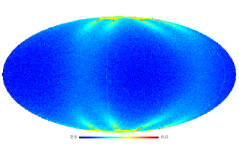
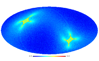
Figure 1: Number of hits per pixel ($n_{\mathrm{hit}}$) for the scan strategy applied in this study. The hit map is shown in the ecliptic (left) and galactic (right) coordinates. The latter map shows the areas of the ecliptic poles more clearly. Both maps include the hits of all four LFI 30 GHz detectors. The scale is $\log_{10}(n_{\rm{hit}})$. (The original version of this paper with better-quality figures is available at www.helsinki.fi/~tfo_cosm/tfo_planck.html .)

3.2 Telescope beams

We assumed identical, circularly symmetric Gaussian telescope beams for every detector. The FWHM of the beams was 32.^′19. There are two 30 GHz feed horns (with two detectors corresponding to two polarisation directions per horn). A coordinate system is defined for each detector, with $z$-axis along the direction of the beam center and $x$ and $y$-axes perpendicular to the pointing, called the main beam coordinate system. The spin 0 and $\pm$2 spherical harmonic coefficients ($b_{\ell m}$ and ${}_{\pm 2}b_{\ell m}$) of the beam response at the reference pointing and orientation were generated for multipoles up to $\ell_{\rm max}$ = 3000 (Challinor et al. challinor00 (2000); Reinecke et al. reinecke06 (2006)). The T, E, and B mode coefficients of the beam were obtained as $b_{\ell m}^{\rm T}=b_{\ell m}$, $b_{\ell m}^{\rm E}=-(_{+2}b_{\ell m}+_{-2}b_{\ell m})/2$ and $b_{\ell m}^{\rm B}=i(_{+2}b_{\ell m}-_{-2}b_{\ell m})/2$. The coefficients $b_{\ell m}^{\rm T}$, $b_{\ell m}^{\rm E}$ and $b_{\ell m}^{\rm B}$ are called the beam $b_{\ell m}$ in this study.

3.3 Noise TOD

The instrument noise was a sum of white and correlated $1/f$ noise. The power spectral density (PSD) of the noise was

$$P(f)=\left[1+\left(\frac{f_{\rm k}}{f}\right)^{\alpha}\right]\frac{\sigma^{2}}{f_{\mathrm{s}}},\quad(f>f_{\mathrm{min}}),$$ (1)

where $f_{\rm k}$ is the knee frequency, i.e., the frequency at which the $1/f$ and white noise are equal, $f_{s}$ is the sampling frequency, and $\sigma$ is the nominal white noise standard deviation per sample integration time ($t=1/f_{\mathrm{s}}$). Below $f_{\rm min}$ the noise spectrum becomes flat. (A $1/f$ spectrum extending to $f=0$ is unphysical.) The spectral slope of the correlated part of the noise is given by $\alpha$. The values of the noise parameters used in this study were: $f_{\rm k}$ = 0.05 Hz, $f_{\rm min}=1.15\times 10^{-5}$ Hz, $\sigma$ = 1350 $\mu$K (CMB scale) and $\alpha$ = 1.7. They represent realistic expected noise performance of the instrument. We used the stochastic differential equation (SDE) algorithm (from Level-S) to generate the TODs of the instrumental noise. The noise samples were generated in 6-day chunks with no correlation between the chunks. No correlation was assumed between the noise TODs of different detectors. For the GLS and Madam map-making codes, perfect knowledge of the above noise parameter values was assumed in the map-making phase.

3.4 Dipole

The temperature Doppler shift that arises from the (constant) motion of the solar system relative to the last scattering surface was included. The Doppler shift arising from the satellite motion relative to the Sun was not included.

3.5 CMB and foregrounds

The CMB and foreground emissions of the sky were modelled with the sets of spherical harmonic coefficients $a_{C,\ell m}^{\rm T,E,B}$ and $a_{F,\ell m}^{\rm T,E,B}$. Here C (F) refers to the CMB (foreground), T refers to the temperature, and E and B refer to the polarisation modes. These expansion coefficients are called sky $a_{\ell m}$ in this study. The sky $a_{\ell m}$ were determined for multipoles up to $\ell_{\rm max}$ = 3000.

The expansion coefficients obtained by convolving the sky $a_{\ell m}$ with the beam $b_{\ell m}$ are called the input $a_{\ell m}$. The map (for the Stokes parameters I, Q and U) made from the input $a_{\ell m}$ is called the input map in this study.

In this section we describe how the CMB and foreground signals were simulated for 30 GHz. In this work the foreground signal is the sum of unresolved extragalactic components and diffuse emission from the Galaxy. These signals are represented as template maps with 1.^′7 pixel size ($N_{\rm side}=2048$). The coefficients $a_{F,\ell m}^{\rm T,E,B}$ were determined from the foreground template map using the anafast code of the HEALPix package.

3.5.1 CMB

The CMB pattern is the same that we used in our earlier study (Ashdown et al. ashdown06 (2006)).

For the total intensity at $\ell\leq 70$, the $a_{C,\ell m}^{\rm T}$ coefficients were taken directly from the output of the anafast code running on the WMAP internal linear combination (ILC) CMB template (Bennett et al. bennett03b (2003)). The coefficients of the E mode polarization, $a_{C,\ell m}^{\rm E}$, at $\ell\leq 70$, were obtained as

$$a_{C,\ell m}^{\rm E}=a_{C,\ell m}^{\rm T}\cdot\frac{C_{\ell}^{\rm TE}}{C_{\ell}^{\rm TT}}+\left(\frac{x_{\ell m}+iy_{\ell m}}{\sqrt{2}}\right)\cdot\sqrt{C_{\ell}^{\rm EE}-\frac{C_{\ell}^{\rm TE}}{C_{\ell}^{\rm TT}}C_{\ell}^{\rm TE}},$$ (2)

where $C_{\ell}^{\rm XY}$ (X,Y = T,E) is the best fit angular power spectrum to the WMAP, ACBAR, and CBI data. The quantities $x_{\ell m}$ and $y_{\ell m}$ are Gaussian distributed random variables with zero mean and unit variance. The imaginary part ($y_{\ell m}$) and the $\sqrt{2}$-factor were not used for $m=0$.

At small angular scales ($\ell>70$), the $a_{C,\ell m}^{\rm T,E}$ coefficients were a random realization of $C_{\ell}^{\rm XY}$ (using the spectrum-to-alm mode of the synfast code of the HEALPix package).

More accurate representations of the CMB are available (e.g., O’Dwyer et al. odwyer04 (2004)), but small differences in the input sky are unimportant for our purposes.

3.5.2 Extragalactic emission

At 30 GHz, the dominant contributions are given by the radio sources. They have been simulated according to the recent data in total intensity and polarization reaching 20 GHz (see Tucci et al. (2004) and references therein). The information extracted from those observations is entirely statistical. In particular, the flux number counts as a function of frequency, and the distribution of the polarization degree are inferred from the observations. Two populations are considered, namely flat and steep spectrum sources, with total intensity spectral index of $-2$ and $-1.2$, respectively. From the polarization distribution, a polarization degree of 2.7% and 4.8% is adopted to the flat and steep spectrum species, respectively. Finally, the polarization angle is assigned randomly to each source.

3.5.3 Diffuse Galactic emission

At 30 GHz, the relevant emission processes from our own galaxy are synchrotron emission from free electrons spiraling around the Galactic magnetic field, and bremsstrahlung emitted by electrons scattering off hydrogen ions. Thermal emission from dust grains dominates galactic emission above about 70 GHz; we include it here because peaks of dust emission in the galactic plane are relevant even at 30 GHz.

For synchrotron emission we use the model of Giardino et al. (2002). On scales of one degree or larger, the 408 MHz sky (Haslam et al. (1982)) is scaled point by point with a spectral index determined from 408 MHz and 1420 MHz data (Reich & Reich (1986)). Structure is extended to smaller angular scales assuming a power law power spectrum matched in amplitude to the local 408 MHz emission, with $C_{\ell}\sim\ell^{-2}$. For polarization we assume the theoretical maximum value for synchrotron emission of $75\%$, and take the polarization direction from the observations at low and medium galactic latitudes. These measures give a rather high fluctuation level reflecting the small scale structure of the galactic magnetic field (Uyaniker et al. (1999); Duncan et al. duncan99 (1999)), scaling as $\ell^{-2}$ from sub-degree to arcminute scales (Tucci et al. (2002)), and consistent with recent observations at medium galactic latitudes (Carretti et al. (2005)). The template for the polarization angle was obtained by adopting the form above for the angular power spectrum, and assuming a Gaussian distribution.

The intensity of the thermal dust emission is well known at 100 $\mu$m, and can be extrapolated to microwave frequencies using the emissivity and temperature of two thermal components (Finkbeiner et al. (1999)). We used model 8 of Finkbeiner et al. (1999), with emissivities and temperatures fixed across the sky. The polarized emission from the diffuse thermal dust has been detected for the first time in the Archeops data (Benoît et al. benoit04 (2004)), which showed a fractional polarization of 5%. The pattern of the polarization angle is much less certain. It is caused by the magnetized dust grains, which are aligned along the galactic magnetic field (Prunet et al. (1998)). Since the geometry and composition of the dust grains are still very uncertain, the simplest assumption is that the galactic magnetic field is 100% efficient in imprinting the polarization angle pattern to the synchrotron and dust emissions (Baccigalupi baccigalupi03 (2003)).

3.6 Convolution of sky and beam for the TOD

To generate the CMB and foreground TOD, we need to convolve the CMB and foreground skies with the telescope beam for every sample of the TOD. We used the total convolution algorithm originally introduced by Wandelt & Górski wandelt01 (2001) to treat the temperature anisotropies, and generalized for polarisation by Challinor et al. challinor00 (2000). The polarized total convolution algorithm has been implemented as a part of Level-S (Reinecke et al. reinecke06 (2006)).

Specifically, the i^th sample of a detector is represented as

$$s_{i}=\sum_{m^{\prime\prime}=-m_{\rm max}}^{m_{\rm max}}\sum_{m,m^{\prime}=-\ell_{\rm max}}^{\ell_{\rm max}}{T_{mm^{\prime}m^{\prime\prime}}e^{i(m\varphi_{i}+m^{\prime}\theta_{i}+m^{\prime\prime}\psi_{i})}},$$ (3)

where ($\theta_{i},\varphi_{i}$) are the spherical coordinates of the pointing of the i^th sample. The angle from the $\mathbf{e}_{\theta}$ axis to the x-axis of the main beam coordinate system is $\psi_{i}$. The largest multipole of the sky $a_{\ell m}$ and the beam $b_{\ell m}$ is $\ell_{\rm max}$ ($\ell_{\rm max}$ = 3000 in this study). The largest $m^{\prime\prime}$ (of the beam $b_{\ell m}$) that is required to describe the beam response is $m_{\rm max}$. For the circularly symmetric beam the $m^{\prime\prime}$ values $-2$, 0, and 2 are sufficient to fully describe the convolution (Challinor et al. challinor00 (2000)). The quantity $T_{mm^{\prime}m^{\prime\prime}}$ represents the convolution of the sky with the beam (Reinecke et al. reinecke06 (2006)) and it is determined from the three sets of parameters: sky $a_{\ell m}$’s, beam $b_{\ell m}$’s and an angle $\psi_{\rm pol}$, which is the angle between the x-axis of the main beam coordinate system and the polarisation sensitive direction of the detector. In the i^th sample the angle from the $\mathbf{e}_{\theta}$ axis to the polarisation sensitive direction of the detector is $\psi_{i}+\psi_{\rm pol}$.

The calculation of the samples $s_{i}$ in their true pointings would be an unrealistically tedious task for the typical mission times (12 months in this study). Therefore in the total convolution algorithm the $m$ and $m^{\prime}$ sums of Eq. (3) are first carried out using a 2-dimensional fast Fourier transform (FFT), and the results are tabulated in 2-dimensional equally spaced grids $T_{m^{\prime\prime}}(\theta,\varphi)$, where ($\theta,\varphi$) tabulates the grid intersections. The size of the grid is $[0,\pi]$ in the $\theta$ direction and $[0,2\pi]$ in the $\varphi$ direction. The grid spacing is $\pi/\ell_{\rm max}$ in both directions. For the circularly symmetric beams there are three grids (for $m^{\prime\prime}=-2$, 0, and 2). Because the samples $s_{i}$ are real, $T_{0}(\theta,\varphi)$ is real, and $T_{-2}(\theta,\varphi)$ = $T^{\ast}_{2}(\theta,\varphi)$. For the case of the circularly symmetric beam, the Level-S total convolver software stores three grids: $T_{0}(\theta,\varphi)$ and the real and imaginary parts of $T_{2}(\theta,\varphi)$ (Reinecke et al. reinecke06 (2006)). These grids are called the ring sets in Level-S.

Level-S uses polynomial interpolation to determine the ring set value at a given pointing from the tabulated values. After the interpolation the final TOD sample value is calculated as

$$\tilde{s}_{i}=\widetilde{T}_{-2}(\theta_{i},\varphi_{i})e^{-i2\psi_{i}}+\widetilde{T}_{0}(\theta_{i},\varphi_{i})+\widetilde{T}_{2}(\theta_{i},\varphi_{i})e^{i2\psi_{i}}.$$ (4)

The symbol $\tilde{s}_{i}$ is used for the calculated TOD sample to indicate that it is an approximation (due to the interpolation) of the true sample value $s_{i}$ (see Eq. (3)). In Eq. (4), $\widetilde{T}_{m^{\prime\prime}}(\theta_{i},\varphi_{i})$ is the ring set value interpolated from the tabulated ring set values. The relation between the ring set values and the Stokes parameters is

$$\widetilde{T}_{0}(\theta_{i},\varphi_{i})=\widetilde{I}(\theta_{i},\varphi_{i})\quad\quad\widetilde{T}_{2}(\theta_{i},\varphi_{i})=\frac{1}{2}\left(\widetilde{Q}(\theta_{i},\varphi_{i})-i\widetilde{U}(\theta_{i},\varphi_{i})\right)e^{i2\psi_{\rm pol}}$$ (5)

Inserting these into Eq. (4) leads to the standard formula for the TOD sample

$$\tilde{s}_{i}=\widetilde{I}(\theta_{i},\varphi_{i})+\widetilde{Q}(\theta_{i},\varphi_{i})\cos{[2(\psi_{i}+\psi_{\rm pol})]}+\widetilde{U}(\theta_{i},\varphi_{i})\sin{[2(\psi_{i}+\psi_{\rm pol})]}.$$ (6)

The interpolation error causes $\widetilde{I}$, $\widetilde{Q}$ and $\widetilde{U}$ to deviate from the Stokes parameters of the input map. It was discovered in earlier studies that a high-order interpolation is required to make this error sufficiently small. Accordingly, we used 11^th order polynomial interpolation when producing the CMB and foreground TODs for this study. The interpolation error that we make is demonstrated in Sect. 3.7.

3.7 Verification

To assess the effects that are present in the (noiseless) CMB and foreground TODs, we compared three CMB maps and three foreground maps. The maps were the input map, ring set map and the binned noiseless map. We used two map resolutions for the comparisons, $N_{\rm side}=512$ and $N_{\rm side}=1024$.

The input maps were discussed in Sect. 3.5.

The ring set map is obtained by interpolating the ring set values ($\widetilde{T}_{0}(\theta_{i},\varphi_{i})$ and $\widetilde{T}_{2}(\theta_{i},\varphi_{i})$) of the HEALPix pixel centers from the tabulated ring set values and then solving the corresponding Stokes parameters $\widetilde{I}(\theta_{i},\varphi_{i})$, $\widetilde{Q}(\theta_{i},\varphi_{i})$ and $\widetilde{U}(\theta_{i},\varphi_{i})$ (see Eq. (5)). The pixel triplets ($\widetilde{I}$, $\widetilde{Q}$, and $\widetilde{U}$) made the ring set map. It is expected that the difference between the ring set map and the input map is mainly caused by the interpolation error. As in the TOD generation, we used 11^th order polynomial interpolation to produce the ring set maps. The ring set maps of this study were made from the ring sets of the detector LFI-27a. It was verified that the ring sets of the other detectors produced identical ring set maps.

The binned noiseless map is obtained by binning the TOD samples in the map pixels

$$\mathbf{m}^{\rm B}=(\mathbf{P}^{\rm T}\mathbf{P})^{-1}\mathbf{P}^{\rm T}\tilde{\mathbf{s}},$$ (7)

where $\mathbf{P}$ is the pointing matrix. It describes the linear combination coefficients for the (I,Q,U) pixel triplet to produce a sample of the observed TOD. Each row of the pointing matrix has three non-zero elements. The vector $\tilde{\mathbf{s}}$ is the simulated signal TOD (CMB or foreground, see Eq. (6)). The pointing matrix used here will produce a binned noiseless map that is smoothed with the telescope beam. The maps were binned from the observations of all four detectors. The polarisation directions were well sampled in each pixel of the $N_{\rm side}=512$ map, leading to 100% sky coverage and rcond $\geq$ 0.2165 over the pixels. For the $N_{\rm side}=1024$ binned noiseless maps we discarded the pixels with no hits or pixels with rcond $<$ 0.01. This led to 912,968 unobserved pixels (out of 12,582,912 pixels of the $N_{\rm side}=1024$ map).

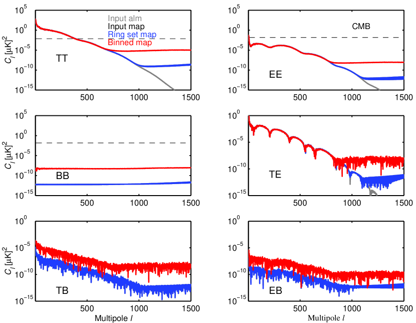
Figure 2: Angular power spectra of the CMB maps ($N_{\rm side}=512$): input map (black curve, not visible since it is so close to the blue curve), ring set map (blue curve) and the binned noiseless map (red). The angular power spectrum of the input $a_{\ell m}$ is shown as well (gray curve). It was calculated in the standard way $C_{\ell}^{\rm in}=\sum_{m=-\ell}^{\ell}|a_{\ell m}^{\rm in}|^{2}/(2\ell+1)$, where $a_{\ell m}^{\rm in}$ are the input $a_{\ell m}$. The horizontal dashed lines give the approximate spectrum of the white noise map (representing 4 detectors). The absolute values of the cross correlation spectra are displayed. The units are CMB microkelvins.

The angular power spectra of the CMB and foreground maps are shown in Figs. 2 and 3 (for $N_{\rm side}=512$). The spectrum of the input $a_{\ell m}$ is shown in gray. The spectra of the input maps and the ring set maps are so close to each other that they cannot be distinguished in the figures (blue curves). The $a_{\ell m}$ coefficients of the input map were produced using the spherical harmonic transform (involving numerical integration) over the pixelized celestial sphere. This discretisation causes a quadrature error in the numerical integration (Górski et al. 2005b ), which shows up as a high-$\ell$ error floor in the spectrum of the input map. Therefore the spectrum of the input map deviates from the spectrum of the input $a_{\ell m}$ at $\ell\gtrsim 1000$. Decreasing the pixel size will decrease the error floor. For the $N_{\rm side}=1024$ input map the quadrature error floor will deviate from the spectrum of the input $a_{\ell m}$ at $\ell\gtrsim 1100$. The high-$\ell$ behavior of the spectrum of the ring set map is also determined by the quadrature error. Therefore the high-$\ell$ error floor of that spectrum is nearly identical to the high-$\ell$ error floor of the spectrum of the input map.

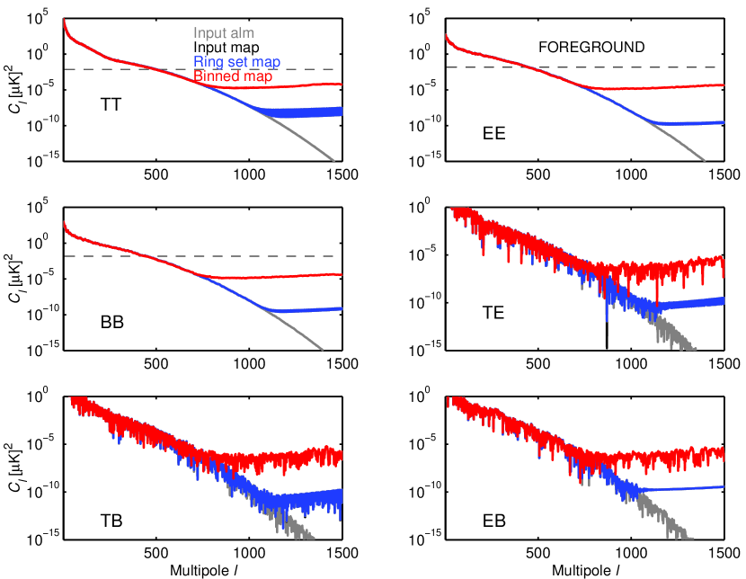
Figure 3: Same as Fig. 2 but the spectra are for foreground maps.

The difference between the ring set maps and the input maps is an indication of the interpolation error that we make in Level-S (see Sect. 3.6). The rms of those difference maps are shown in the first row of Tables 1 and 2. The difference is very small.

The object of interest in the sky maps is their anisotropy, and the mean sky temperature is irrelevant. Therefore, whenever we calculated a map rms in this study, we subtracted the mean of the observed pixels from the map before squaring. The rms of a map was always calculated over the observed pixels only.

We also calculated the ratio of the spectra of the $N_{\rm side}=512$ ring set maps and the input maps. Those ratios are shown in Figs. 4 and 5 (blue curves). The spectra are nearly identical. Note, however, that at $\ell\gtrsim 1000$ the spectra are determined by the quadrature error of the numerical integration and the ratios do not reflect the interpolation errors at those $\ell$. Based on the difference maps and the spectrum ratios, we conclude that the 11^th-order polynomial interpolation that we used in Level-S causes insignificant error in the simulated TODs.

	rms $[\mu$K$]$ ($N_{\rm side}=512$)			rms $[\mu$K$]$ ($N_{\rm side}=1024$)
Map difference	I	Q	U	I	Q	U
Ring set - input	4.070$\times$10-6	5.786$\times$10-8	5.149$\times$10-8	4.070$\times$10-6	5.771$\times$10-8	5.146$\times$10-8
Binned - input	1.472	0.0451	0.0458	2.291	0.0768	0.0780
Binned - pix convolved input	1.401	0.0415	0.0422

Table 1: Rms of the CMB difference maps. All the $N_{\rm side}=512$ maps and the $N_{\rm side}=1024$ input and ring set maps cover the full sky, whereas the $N_{\rm side}=1024$ binned noiseless map has 912,968 missing pixels (unobserved or with $rcond<0.01$). The rms of the difference maps was determined over the pixels observed by both maps. The order of the polynomial interpolation is 11 for the ring set maps. For comparison, the rms of the CMB input map is (I,Q,U) = (84.2, 1.02, 1.03) $\mu$K. (The rms of the input map after the convolution with the $N_{\rm side}=512$ HEALPix pixel window function is (I,Q,U) = (84.0, 1.00, 1.02) $\mu$K.). The units are CMB microkelvins.

	rms $[\mu$K$]$ ($N_{\rm side}=512$)
Map difference	I	Q	U
Ring set - input	3.639$\times$10-5	7.286$\times$10-6	7.239$\times$10-6
Binned - input	2.933	2.5122	2.570

Table 2: Same as Table 1, but this is for the $N_{\rm side}=512$ foreground maps. The rms of the foreground input map is (I,Q,U) = (599.8, 135.3, 133.8) $\mu$K.

The pixel (I,Q,U) triplet of the binned noiseless map represents (approximately) the mean of the observations falling in that pixel, whereas the pixel (I,Q,U) of the input map represents an observation from the pixel center. The non-uniform scatter of observations in the output map pixels makes the spectrum of the binned noiseless map different from the spectrum of the input map in two distinct ways. The scatter of observations causes a spectral smoothing and leads to an $\ell$ mode coupling (Poutanen et al. poutanen06 (2006)).

The angular spectra of the binned noiseless maps are shown in Figs. 2 and 3 (red curves, for $N_{\rm side}=512$). The spectral smoothing is not visible there, but the high-$\ell$ flat plateau caused by the $\ell$ mode coupling can be seen clearly. The plateau is produced when the power from low $\ell$ (where there is lot of power) is coupled to high $\ell$ (low power) as a result of the $\ell$-mode coupling. The WMAP team discusses this issue in their 3-year data analysis and uses the term aliasing for $\ell$-mode coupling (Jarosik et al. jarosik06 (2006)). In this study, the flat spectrum plateau of the $\ell$ mode coupling is called the aliasing error. Because the two detectors of a horn have identical circularly symmetric beams and identical pointings, the high-$\ell$ plateau of the EE and BB spectra is not caused by the total intensity leaking to polarisation, rather the EE and BB plateaus are the result of the $\ell$-mode couplings of the E and B mode polarisations.

The horizontal dashed lines of Figs. 2 and 3 indicate the approximate level of the white noise (arising from the four detectors). At $N_{\rm side}=512$ the aliasing error (plateau) is clearly smaller than the instrument noise. If the pixel size is increased, the difference between the noise spectrum and the aliasing error will decrease, because the increased pixel size will increase the aliasing error, but the level of the noise spectrum remains nearly unaffected. We made a binned noiseless foreground map for $N_{\rm side}$ = 64. Its aliasing error had nearly the same value as the spectrum of the $N_{\rm side}$ = 64 white noise map.

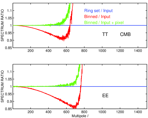
Figure 4: Ratios of some of the spectra shown in Fig. 2. For the green curve the spectrum of the binned noiseless map was deconvolved with the $N_{\rm side}=512$ HEALPix pixel window function before calculating the ratio.

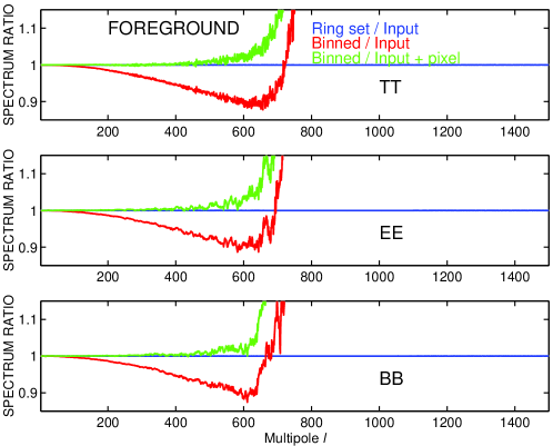
Figure 5: Ratios of some of the spectra shown in Fig. 3. For the green curve the spectrum of the binned noiseless map was deconvolved with the $N_{\rm side}=512$ HEALPix pixel window function before calculating the ratio.

The spectral smoothing due to the scatter of observations is demonstrated in Figs. 4 and 5. The ratios of the spectra of the binned noiseless map and the input map are shown (red curves, for $N_{\rm side}=512$ maps). For $\ell\lesssim 600$, the spectral smoothing can be well modelled with the HEALPix pixel window function (Górski et al. 2005b ). We recalculated the ratios after the spectrum of the binned noiseless map had been deconvolved with the $N_{\rm side}=512$ HEALPix pixel window function. The resulting ratios are shown as well (green curves). They show, that, in this case, the spectra (of input map, ring set map and pixel window deconvolved binned noiseless map) are nearly identical at low $\ell$ ($\ell\lesssim 400$). The blow-up of the ratios at $\ell\approx 700$ is due to the aliasing error.

The rms of the difference between the binned noiseless maps and the input maps is shown in Tables 1 and 2. It contains the effects of both spectral smoothing and mode coupling. To remove (approximately) the effect of spectral smoothing we smoothed the input map with the HEALPIx pixel window function, and then recalculated the difference. The resulting rms is shown in the third row of Table 1 (this was done for the $N_{\rm side}=512$ CMB input map only). Comparing the second and the third rows of Table 1, we see that the aliasing error (the high-$\ell$ plateau) is the main contributor in the difference between the binned noiseless map and the input map.

The main purpose of this paper is to compare map-making algorithms. We want to isolate errors introduced in the map-making process from the imperfections (e.g., the scatter of the observations) of the experimental setup. The difference between the output map and the input map includes the experimental effects, whereas the difference between the output map and the binned noiseless map is essentially free of them. Therefore we will examine the latter difference maps in the remaining parts of this paper.

4 Results

Simulated TODs for CMB, dipole, foregrounds, and noise were made individually for the four LFI 30 GHz detectors. Maps and angular power spectra made from combinations of these TODs are discussed below. Most of our output maps had $\sim$7 arcmin ($N_{\rm side}=512$) pixel size. At this resolution the polarisation directions were well sampled in every pixel of the map (see Sect. 3.7).

MapCUMBA, MADmap, ROMA, and Madam applied the known PSD of the instrument noise (see Sect. 3.3). In a real experiment, of course, the noise properties must be estimated from the observed data. Here we wanted to avoid the errors that would arise if we used estimated noise PSDs instead of the actual one. The length of the uniform baselines was 1 min in Polar and 1.2 s in Madam. For comparison, Madam was also run in some cases with longer 1 min uniform baselines. Whenever we discuss Madam in this paper without specifying the baselines, 1.2 s baselines are assumed.

The top row of Fig. 6 shows the typical output map (temperature and polarization) made from the full simulated data (CDFN = CMB + dipole + foreground + noise), and the black curves in Fig. 7 show the angular power spectra of this output map. The red curves in Fig. 7 show the corresponding spectra for the noiseless (CDF) case. For comparison we show the spectrum of the input $a_{\ell m}$ too (for CDF and for CMB alone). We see that the CDFN output map is signal-dominated at large angular scales ($\ell\lesssim 400$) and noise-dominated at small angular scales. The output map shown is from Polar, but the output maps and their angular power spectra from all six map-making codes would look the same in these figures. To bring out the differences we consider various difference maps and their spectra.

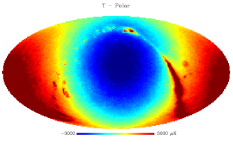
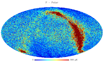
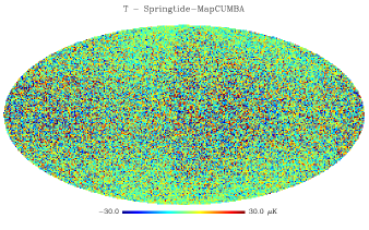
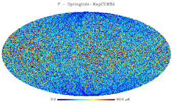
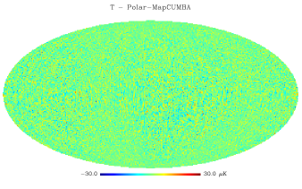
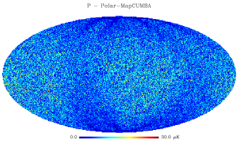
Figure 6: Top row: CDFN output map of Polar. Middle row: CDFN difference map of Springtide and MapCUMBA. Bottom row: CDFN difference map of Polar and MapCUMBA. These $N_{\rm side}=512$ maps contain CMB, dipole, foregrounds, and noise (CDFN). They are displayed in ecliptic coordinates. The left hand maps are Stokes I, and the right hand maps are for the magnitude $P$ of the polarisation vector ($P=\sqrt{Q^{2}+U^{2}}$). The map units are CMB microkelvins. Note the different color scales of the two bottom $P$ maps. (See www.helsinki.fi/~tfo_cosm/tfo_planck.html for better-quality figures.)

As a first step in characterizing the differences between the map-making codes, we calculated the pairwise differences between their output maps. These difference maps are dominated by the difference in the remaining noise in these output maps. The rms of these difference maps are given in Table 3. We see that the differences between the output maps of the three GLS codes, as well as Madam, are relatively small. The Polar and Springtide maps are more different. We confirm in Sect. 4.1 that the GLS maps contain less noise than the Polar and Springtide maps.

$N_{\rm side}=512$, rms $[\mu$K$]$	Springtide	Polar	Madam	ROMA	MADmap	MapCUMBA
Springtide		14.061	14.609	14.634	14.628	14.628
Polar	19.845		4.042	4.116	4.104	4.104
Madam	20.615	5.712		0.729	0.601	0.596
ROMA	20.658	5.849	1.169		0.409	0.415
MADmap	20.642	5.801	0.833	0.822		0.074
MapCUMBA	20.642	5.800	0.822	0.830	0.135

Table 3: Rms of the differences of the CDFN output maps. The data in the upper right triangle are for the I difference maps. The values in the lower left triangle are obtained as $\sqrt{(\sigma_{\rm Q}^{2}+\sigma_{\rm U}^{2})/2}$, where $\sigma_{\rm Q}$ and $\sigma_{\rm U}$ are the rms of the Q and U difference maps. The maps had $N_{\rm side}=512$ and the units are CMB microkelvins.

The Springtide $-$ MapCUMBA and Polar $-$ MapCUMBA difference maps are shown as the middle and bottom rows of Fig. 6. Some large scale structure (stripes along the scan path) is (barely) visible in the Polar $-$ MapCUMBA difference map. These stripes reflect the difference in the residual $1/f$ noise in the output maps. Similar large scale structure is not visible in the Springtide $-$ MapCUMBA difference map because of the higher pixel scale noise in the Springtide output map. The rms of the Polar $-$ GLS difference maps is only $\sim$$1/3.5$ of the rms of the Springtide $-$ GLS difference maps. The reason for the large Springtide $-$ GLS output map difference is the high-$\ell$ residual noise of the Springtide maps as discussed below.

The angular power spectra of the Springtide $-$ MapCUMBA and Polar $-$ MapCUMBA CDFN difference maps are shown in Fig. 8. We see from these spectra that the Springtide and Polar output maps have similar noise structure (stripes) at large angular scales (low $\ell$), but for Springtide more noise remains at high $\ell$. This high-$\ell$ noise shows up as pixel scale noise in the difference map (see Fig. 6). Fig. 8 shows the angular spectrum of the Madam $-$ MapCUMBA CDFN difference map too. It is clearly smaller than the other difference map spectra of Fig. 8, showing that the noise of the Madam output map approaches the noise of the GLS output maps.

Fig. 8 further shows, that the CMB temperature anisotropy signal is larger than the residual noise at low and intermediate multipoles ($\ell\lesssim 400$, top panel). The residual noise differences (of different map-making codes) are tiny fractions of the CMB temperature signal in those multipoles. In the polarization maps the residual noise differences are of the same order of magnitude as the CMB signal (middle panel), which is now significantly smaller than the residual noise and thus difficult to detect.

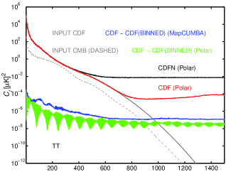
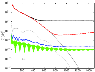
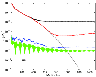
Figure 7: Angular power spectra of the Polar output CDFN (CMB+dipole+foreground+noise) map (black) and some noiseless (CDF) maps. All maps are full sky $N_{\rm side}=512$ maps . INPUT CDF (gray) is the spectrum of the sum of the input $a_{\ell m}$ of CMB, foreground and dipole. INPUT CMB (gray, dashed) is the spectrum of the input $a_{\ell m}$ of the CMB alone. Note that input $a_{\ell m}^{\rm B}=0$ for the CMB. CDF (red) is the same as the black curve but with no noise. Blue and green curves are the spectra of the difference maps CDF $-$ CDF(binned), where CDF(binned) is the binned noiseless map of CDF. Blue curve is for MapCUMBA and green curve is for Polar. The units are CMB microkelvins.

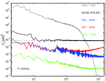
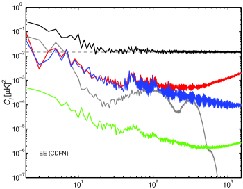
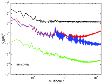
Figure 8: Angular power spectra of the CDFN difference maps. The red curve is for the difference of the Springtide (SPT) and MapCUMBA (MCB) output maps, the blue curve is for the difference of Polar (POL) and MapCUMBA output maps and the green curve is for the difference of the Madam (MDM) and MapCUMBA output maps. All maps were $N_{\rm side}=512$ maps and the units are CMB microkelvins. For comparison we show the spectra of the CMB input $a_{\ell m}$ (gray curve) and the noise only output map of Polar (black curve). The horizontal dashed line is an approximation of the spectrum of the white noise map (see the caption of Table 4).

The output map from map-making can be represented as a sum of three components (Poutanen et al. poutanen06 (2006)): the binned noiseless map, the residual noise map, and an error map that arises from the small scale (subpixel) signal structure that couples to the output map through the map-making. This error map is called the signal error map in this study. The binned noiseless map is the map we want and the residual noise map and signal error map are unwanted errors that depend on the map-making algorithm used.

4.1 Residual noise maps

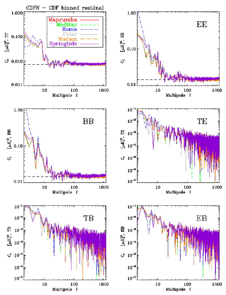
Figure 9: Angular power spectra of the difference maps: CDFN output map $-$ CDF binned noiseless map. The maps covered the full sky and their resolution was $N_{\rm side}=512$. The units are CMB microkelvins. The horizontal dashed lines in the TT, EE and BB spectrum plots show the expected angular spectrum of the white noise map. (See www.helsinki.fi/~tfo_cosm/tfo_planck.html for better-quality figures.)

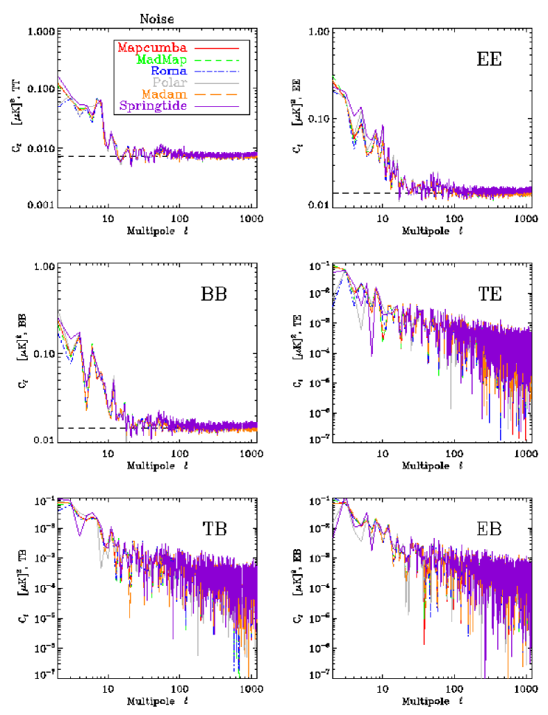
Figure 10: Angular power spectra of the residual noise maps (noise only output maps). The maps covered the full sky and their resolution was $N_{\rm side}=512$. The units are CMB microkelvins. The horizontal dashed lines in the TT, EE and BB spectrum plots show the expected angular spectrum of the white noise map. (See www.helsinki.fi/~tfo_cosm/tfo_planck.html for better-quality figures.)

We computed the total error map (sum of residual noise and signal error maps) by subtracting the binned noiseless map from the output map. The angular power spectra of the CDFN total error maps are shown in Fig. 9. These spectra were compared to the angular power spectra of the residual noise maps, shown in Fig. 10. The residual noise map is made from the noise TOD only. The residual noise dominates the total error in the CDFN case. Therefore the spectra of Figs. 9 and 10 are nearly identical. The spectra contain significant structure at low $\ell$, but tend towards the white noise plateau at $\ell\gtrsim 20$ (the expected spectra of the white noise map are shown as dashed horizontal lines). Figs. 9 and 10 show small differences between the spectra of different map-making methods. The ROMA EE and BB spectra of the total error are exceptions. They have somewhat larger power at low $\ell$ than the other spectra. We could probably have let the ROMA code to perform some more conjugate gradient iterations for better recovery of the low-$\ell$ power.

The rms of the residual noise maps (white + $1/f$) and the approximate level of the $1/f$ noise are given in Table 4. Since map-making algorithms suppress $1/f$ noise, the magnitude of the residual $1/f$ noise is a good metric for code comparison. The Polar map contains more residual $1/f$ noise than the maps of the GLS codes (MapCUMBA, MADmap and ROMA). The difference is, however, small. The Madam map for 1 min uniform baselines has the same residual noise as the Polar map. When using short uniform baselines (1.2 s), Madam can produce maps with as low residual noise as the GLS codes.

Springtide requires less computing resources than the other codes, but residual noise from Springtide is higher because it works with long (1 hr) ring baselines rather than with the shorter baselines used in Polar (1 min) and Madam (1.2 s). The higher residual $1/f$ noise of Springtide shows up as a higher map noise (especially at high $\ell$, as can be seen in Figs. 6 and 8). The larger high-$\ell$ noise of Springtide is also (barely) visible in the spectra of Figs. 9 and 10.

Table 4 shows that in the output maps the amount of residual $1/f$ noise power is 11.6% (Springtide), 1.9% (Polar), and 0.9% (Madam and GLS codes) of the overall residual noise power.

$N_{\rm side}=512$	Res. noise, rms $[\mu$K$]$			Res. $1/f$ noise, rms $[\mu$K$]$
Code	I	Q	U	I	Q	U
Polar	43.02	60.73	61.26	5.78	7.85	7.65
Springtide	45.25	63.84	64.41	15.17	21.19	21.32
Madam (1 min)	43.02	60.73	61.25	5.78	7.85	7.57
Madam (1.2 s)	42.83	60.46	60.99	4.13	5.38	5.06
MapCUMBA	42.83	60.46	60.98	4.13	5.38	4.93
MADmap	42.83	60.46	60.98	4.13	5.38	4.93
ROMA	42.83	60.46	60.98	4.13	5.38	4.93
White noise	42.63	60.23	60.78
CMB	84.21	1.02	1.03

Table 4: Pixel statistics of the residual noise maps (output maps of the noise-only TOD) are shown in the left columns of the table. The residual noise is a sum of residual white and $1/f$ noise. For comparison, the rms of the CMB input map and an approximate rms of a white noise map are also shown. The actual number of hits and the sampling of the polarisation directions were considered for every pixel when the white noise rms was computed. The right columns of the table give an approximate level of the residual $1/f$ noise of the output maps. It is calculated as $\sqrt{\sigma_{\rm n}^{2}-\sigma_{\rm wn}^{2}}$, where $\sigma_{\rm n}$ is the rms of the residual noise (from the left columns) and $\sigma_{\rm wn}$ is the rms of the white noise (from the second bottom row of the table). The units are CMB microkelvins.

4.2 Signal error maps

If we bin the noiseless signal TOD to a map, scan that map back to TOD, and subtract it from the original TOD, the resulting difference TOD gives the pixelisation noise (Doré et al. dore01 (2001)). It was shown in Poutanen et al. poutanen06 (2006) that the pixelisation noise is the source of the signal error map. Assuming a sum of CMB, dipole, and foreground signals, four LFI 30 GHz detectors, 12 months mission time, and $N_{\rm side}=512$, we estimated the rms of the pixelisation noise. Its value was only about 1% of the white noise rms ($\sigma$) of a TOD sample (see Sect. 3.3). Therefore the residual noise dominates the total error for $N_{\rm side}=512$ maps.

In GLS map-making, the pixelisation noise spectrum up to the knee frequency of the instrument noise contributes to the signal error map, whereas in destriping only the uniform baselines of the pixelisation noise contribute (Hivon et al. hivon06 (2006); Poutanen et al. poutanen06 (2006)). Therefore we expect that the Polar and Springtide output maps (with their longer baselines) will have smaller signal error than the GLS output maps. The signal error of the Madam map (with its short baselines) should approach the signal error of the GLS maps.

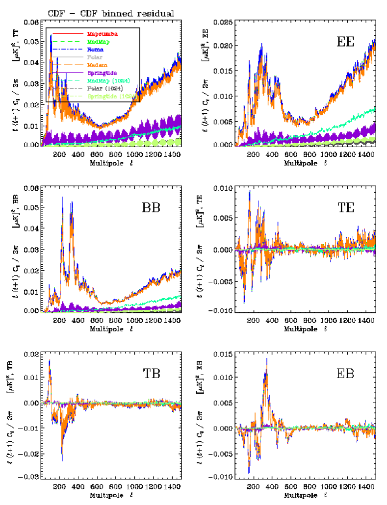
Figure 11: Same as Fig. 9, but now for noiseless (CDF) output maps. All $N_{\rm side}=512$ maps were full sky maps. Due to no observations or poor sampling of the polarisation directions the $N_{\rm side}=1024$ maps contained a number of unobserved pixels (see Table 7). (See www.helsinki.fi/~tfo_cosm/tfo_planck.html for better-quality figures.)

The signal error map can be obtained by subtracting the binned noiseless map from the signal-only output map. The angular power spectra of the MapCUMBA and Polar signal error maps (for $N_{\rm side}=512$) are shown in Fig. 7. The corresponding spectra of the other GLS codes and Madam would be nearly identical to the MapCUMBA spectrum, whereas the Springtide spectrum would be more like the Polar spectrum. As expected, the GLS signal error is clearly larger than the signal error of destriping. The full set of spectra of the $N_{\rm side}=512$ signal error maps is shown in Fig. 11.

The pixel statistics of the $N_{\rm side}=512$ signal error maps for a sum of CMB, dipole, and foreground (CDF) are shown in Table 5. Polar and Springtide maps have nearly the same levels of signal error. These levels are smaller than the levels of the GLS and Madam maps. The peak signal error of the Madam map for 1 min uniform baselines is larger than the peak errors of the Polar and Springtide maps, although the error rms are nearly the same.

The levels of the signal error are significantly smaller than the levels of the residual noise (in $N_{\rm side}=512$ output maps). However, the peak signal errors of Table 5 (especially the errors of the GLS and Madam maps) approach or exceed 3 $\mu$K, which is the LFI performance goal of the maximum systematic error per pixel (see Table 1.2 in p. 8 of the ”Planck Bluebook”: Efstathiou et al. efstathiou05 (2005)). We need also to compare the rms of the signal error (left columns of Table 5) to the rms of the residual $1/f$ noise (right columns of Table 4). For the GLS codes the signal error can be up to $\sim$7.4% of the residual $1/f$ noise. For the other map-making codes the relative magnitude of the signal error is smaller.

We examined the signal error maps separately for CMB, dipole, and foreground. The resulting statistics are shown in Table 6. As expected, the foreground signal (a sum of signals from our own galaxy and extra-galactic point sources) is the strongest contributor in the signal error map.

$N_{\rm side}=512$	CDF - CDFbin, rms $[\mu$K$]$			max - min $[\mu$K$]$
Code	I	Q	U	I	Q	U
Polar	$0.143$	$0.0746$	$0.0775$	$2.46$	$1.31$	$1.38$
Springtide	$0.142$	$0.0744$	$0.0771$	$2.39$	$1.98$	$1.37$
Madam	$0.290$	$0.185$	$0.208$	$11.90$	$7.94$	$9.85$
Madam (1 min)	$0.143$	$0.0754$	$0.0783$	$5.92$	$3.64$	$4.16$
MapCUMBA	$0.305$	$0.193$	$0.218$	$14.00$	$8.50$	$10.00$
MADmap	$0.304$	$0.193$	$0.218$	$14.00$	$8.50$	$10.00$
ROMA	$0.305$	$0.193$	$0.218$	$14.00$	$8.50$	$10.00$

Table 5: Pixel statistics of the noiseless difference maps: output map $-$ binned noiseless map. Maps contained CMB, dipole, and foreground (CDF) and they were full sky maps with $N_{\rm side}=512$ resolution. The units are CMB microkelvins.

$N_{\rm side}=512$	CMB, rms [nK]			Dipole, rms [nK]			Foreground, rms [nK]
Code	I	Q	U	I	Q	U	I	Q	U
Polar	$75.9$	$2.53$	$1.92$	$18.7$	$0.170$	$0.181$	$119$	$74.6$	$77.5$
Springtide	$75.7$	$2.53$	$1.92$	$18.6$	$0.170$	$0.181$	$118$	$74.3$	$77.2$
Madam	$143$	$4.75$	$3.69$	$35.5$	$0.174$	$0.213$	$259$	$185$	$208$
MapCUMBA	$148$	$5.11$	$3.90$	$36.9$	$1.97$	$0.646$	$273$	$193$	$218$
MADmap	$148$	$4.96$	$3.77$	$36.8$	$0.621$	$1.36$	$273$	$193$	$218$
ROMA	$148$	$4.92$	$3.74$	$37.3$	$2.85$	$0.94$	$273$	$193$	$218$

Table 6: Pixel statistics of the noiseless difference maps (output map $-$ binned noiseless map) separately for CMB, dipole, and foreground. resolution. Note that the data are now presented in units of CMB nanokelvins.

The signal error maps of Polar and Springtide are binned from uniform baselines that are approximately the baselines of the pixelisation noise. These baselines represent 1 min circles (Polar) or 1 hour rings (Springtide) in the sky. Because the signal errors of the GLS and Madam maps also contain higher frequency components, we expect that their signal error maps will contain more small scale structure than the corresponding maps of Polar and Springtide. The MapCUMBA and Polar signal error maps for CDF are shown in Fig. 12. The largest errors in the MapCUMBA map are located in the vicinity of the galaxy, where the pixelisation noise (signal gradients) is strongest. Such localization of errors does not exist in the destriped maps, because those codes spread the errors that arise from the small-scale signal structure over circles in the sky.

To decrease the signal error, we examined several schemes. They are described in Sect. 4.2.1 - 4.2.4.

4.2.1 Reducing the pixel size of the output map

We expect the mean power of the pixelisation noise to decrease as the pixel size of the output map is decreased. Therefore output maps with smaller pixels should also have a smaller map-making signal error. We examined this assumption by making $N_{\rm side}=1024$ maps from our simulated TODs.

Decreasing the pixel size will also decrease the number of observations falling in them. In our simulations the $N_{\rm side}=1024$ maps had a set of pixels with no observations and another set with poor sampling of the polarisation directions. The latter pixels will have ill-behaving $3\times 3$ block matrices (see the footnote in Sect. 3.7). The residual noise and the signal error of these pixels will be amplified by the inverses of their ill-behaving $3\times 3$ matrices. The quality of the polarisation sampling can be quantified by the rcond value of the $3\times 3$ matrix (see the footnote in Sect. 3.7). We need to set up a lower limit for rcond and discard all pixels that have rcond smaller than this threshold. Our $N_{\rm side}=1024$ output maps had 191,026 pixels (out of 12,582,912 pixels in total) with no observations.

The spectra of the $N_{\rm side}=1024$ CDF difference maps (binned noiseless map subtracted from the noiseless output map) are shown in Fig. 11. We can see from Fig. 11, that decreasing the pixel size (from $N_{\rm side}=512$ to $N_{\rm side}=1024$) decreases the magnitude of the signal error spectrum. The corresponding map domain statistics for $N_{\rm side}=1024$ can be found in Table 7. This table can be compared to Table 5. This comparison shows, that, although the rms of most of the $N_{\rm side}=1024$ signal error maps are smaller (than the rms of the $N_{\rm side}=512$ signal error maps), the peak errors are larger. Large peak errors were most likely produced by some ill-sampled pixels that still remain in the maps.

$N_{\rm side}=1024$	CDF - CDFbin, rms $[\mu$K$]$			max - min $[\mu$K$]$
Code	I	Q	U	I	Q	U
Polar	$0.118$	$0.0722$	$0.0735$	$4.63$	$5.12$	$5.34$
Springtide	$0.112$	$0.0820$	$0.0834$	$4.11$	$11.1$	$11.1$
MADmap	$0.225$	$0.185$	$0.189$	$16.9$	$26.3$	$26.1$

Table 7: Pixel statistics of the noiseless difference maps: output map $-$ binned noiseless map. Maps contained CMB, dipole and foreground (CDF) and their resolution was $N_{\rm side}=1024$. Before computing the statistics we discarded 902,913 pixels from the Polar and MADmap maps and 837,430 pixels from the Springtide map. The rcond threshold used in Polar and MADmap was $\sim$$10^{-2}$, whereas the threshold of the Springtide was $10^{-3}$. The units are CMB microkelvins.

4.2.2 Discarding crossing points in destriping

In destriping, a crossing point is identified, when the samples of two (or more) baselines measure the same sky pixel. The Polar code can ignore crossing points that fall outside a sky mask given by the user. By using a mask that ignores the galactic and point source regions, we can prevent the large signal gradients of these areas from introducing errors in the baseline amplitudes. After computing the baseline amplitudes, we subtract them from the original TOD and bin the output map as before. The output map then contains the observations from the galactic and pointsource regions also.

We used Polar and made $N_{\rm side}=512$ CDF output maps using two different masks for discarding the crossing points. We called the masks Kp0 cut and $\pm$20$\degr$ cut. They are defined in Fig. 13. The pixel statistics of the signal error (CDF $-$ CDFbin difference maps) are shown in Table 8. Kp0 reduces the rms of the signal error by factors $\sim$1.3 (I map) and $\sim$2.0 (Q and U maps). The peak errors are reduced by factors $\sim$1.03 (in I map) and $\sim$2.1 (in Q and U maps). In spite of the fact that $\pm$20$\degr$ cut removes larger galactic regions than Kp0, the signal error of the $\pm$20$\degr$ cut is larger than the signal error of Kp0. When we introduce a galactic cut in the crossing points, the magnitude of the pixelisation noise (signal gradients) becomes smaller, which decreases the signal error. On the other hand, the galactic cut reduces the number of crossing points (from the full sky case) and makes the ”connection” of our observations poorer. A poor connection tends to bring more error in the baselines, which increases the signal error. At some point increase of the extent of the galactic cut does not help anymore and the signal error will not decrease.

$N_{\rm side}=512$	CDF - CDFbin, rms $[\mu$K$]$			max - min $[\mu$K$]$
Polar	I	Q	U	I	Q	U
Kp0	$0.108$	$0.0381$	$0.0371$	$2.39$	$0.68$	$0.60$
$\pm$20$\degr$	$0.124$	$0.0402$	$0.0400$	$3.51$	$0.75$	$0.63$
Full sky	$0.143$	$0.0746$	$0.0775$	$2.46$	$1.31$	$1.38$

Table 8: Pixel statistics of the noiseless difference maps (signal error) of Polar: output map - binned noiseless map. Maps contained CMB, dipole, and foreground (CDF) and they were full sky maps with $N_{\rm side}=512$ resolution. The crossing points of baselines that fall in the galactic or point source regions have been discarded. For comparison we also show the full sky Polar data (all crossing points included). It is the same data as in the first row of Table 5.

We also made noise-only output maps after masking the crossing points. The rms of the residual noise map is larger for Kp0 and $\pm$20$\degr$ cuts than for the noise map with no crossing points discarded, but the difference is small (see Table 9). The goal of destriping is to fit uniform baselines to the $1/f$ component of the detector noise. Galactic cut reduces the number of crossing points and makes the connection of our observations poorer, which leads to a larger fitting error than when all the crossing points are used. Therefore the residual noise is larger for the galactic cuts than for the full sky.

$N_{\rm side}=512$	Res. noise, rms $[\mu$K$]$
Polar	I	Q	U
Kp0	$43.03$	$60.74$	$61.27$
$\pm$20$\degr$	$43.04$	$60.75$	$61.28$
Full sky	$43.02$	$60.73$	$61.26$

Table 9: Pixel statistics of the Polar residual noise maps. The crossing points of baselines that fall in the galactic or point source regions have been discarded. The full sky Polar data (all crossing points included) is the same data as in the first row of Table 4.

4.2.3 Reducing the pixel size of the crossing points in destriping

In destriping we use a pixelized sky to determine the crossing points of two (or more) baselines. The samples of the crossing baselines, that fall in the same pixel, do not necessarily measure the same point in the sky but they may have different pointings. In destriping the signal error arises from the differences of these samples. We expect that reducing the pixel size of the crossing points will lead to smaller sample differences and thus smaller signal error. So far in this paper the destriping codes have used the same pixel size for the crossing points and output maps.

The Polar code has an option, that allows independent pixel sizes for the crossing points and output map. We made a number of $N_{\rm side}=512$ CDF output maps using a different pixel size for the crossing points. The pixel statistics of the signal error (CDF $-$ CDFbin difference maps) are shown in Table 10. It clearly shows, that smaller pixels for the crossing points lead to smaller signal error.

$N_{\rm side}=512$ Output map	CDF - CDFbin, rms $[\mu$K$]$			max - min $[\mu$K$]$
Polar	I	Q	U	I	Q	U
Crossing point pixels
$N_{\rm side}=4096$	$0.0146$	$0.00737$	$0.00756$	$0.31$	$0.17$	$0.14$
$N_{\rm side}=2048$	$0.0335$	$0.0187$	$0.0190$	$0.93$	$0.37$	$0.40$
$N_{\rm side}=1024$	$0.0685$	$0.0364$	$0.0368$	$1.59$	$0.67$	$0.69$
$N_{\rm side}=512$	$0.143$	$0.0746$	$0.0775$	$2.46$	$1.31$	$1.38$
$N_{\rm side}=256$	$0.393$	$0.194$	$0.208$	$5.67$	$3.04$	$3.42$
$N_{\rm side}=128$	$1.217$	$0.570$	$0.600$	$17.92$	$8.50$	$9.38$
$N_{\rm side}=64$	$3.556$	$1.372$	$1.448$	$61.01$	$18.68$	$23.92$

Table 10: Pixel statistics of a number of noiseless difference maps (signal error) of Polar: output map - binned noiseless map. Maps contained CMB, dipole, and foreground (CDF) and they were all full sky maps with $N_{\rm side}=512$ resolution. We used a different crossing point pixel size every time we made a map. We discarded those crossing points that fell in pixels, whose rcond was $<10^{-6}$. The data for the $N_{\rm side}=512$ crossing points is from the first row of Table 5.

We also made noise-only output maps using a different crossing point pixel size every time we made a map. The output map resolution was $N_{\rm side}=512$ in every map. The pixel statistics of these residual noise maps are shown in Table 11 (in the left I,Q,U columns). We also show the approximate rms of the residual $1/f$ noise (in the middle I,Q,U columns). They are determined from the residual noise rms as in Table 4. Smaller crossing point pixels reduce the number of crossing points and therefore make the connection of our observations poorer. It leads to a larger error in the baseline fit (cf. Sect. 4.2.2). Therefore maps with small crossing point pixels have a higher residual noise than the maps with larger crossing point pixels (see Table 11).

We approximated the rms of the total effect (residual $1/f$ noise and signal error) by adding the squares of their rms and taking the square root of the sum. The result is shown in the right I,Q,U columns of Table 11. We can see, that in this case the total effect is at its minimum for $N_{\rm side}=256$ (I) and $N_{\rm side}=128$ (Q,U) crossing point pixels. The minima are not, however, very distinct.

$N_{\rm side}=512$ Output map	Res. noise, rms $[\mu$K$]$			Res. $1/f$ noise, rms $[\mu$K$]$			Res. $1/f$ noise + signal error, rms $[\mu$K$]$
Polar	I	Q	U	I	Q	U	I	Q	U
Crossing point pixels
$N_{\rm side}=4096$	$43.12$	$61.00$	$61.53$	$6.48$	$9.66$	$9.58$	$6.48$	$9.66$	$9.58$
$N_{\rm side}=2048$	$43.08$	$60.84$	$61.37$	$6.21$	$8.59$	$8.49$	$6.21$	$8.59$	$8.49$
$N_{\rm side}=1024$	$43.04$	$60.76$	$61.29$	$5.93$	$8.01$	$7.89$	$5.93$	$8.01$	$7.89$
$N_{\rm side}=512$	$43.02$	$60.73$	$61.26$	$5.78$	$7.78$	$7.65$	$5.78$	$7.78$	$7.65$
$N_{\rm side}=256$	$43.00$	$60.70$	$61.22$	$5.63$	$7.54$	$7.33$	$5.64$	$7.54$	$7.33$
$N_{\rm side}=128$	$42.99$	$60.69$	$61.22$	$5.55$	$7.46$	$7.28$	$5.68$	$7.48$	$7.31$
$N_{\rm side}=64$	$42.99$	$60.69$	$61.21$	$5.55$	$7.46$	$7.24$	$6.59$	$7.58$	$7.39$

Table 11: Pixel statistics of a number of Polar residual noise maps (left I,Q,U columns). All maps had $N_{\rm side}=512$ resolution, but we used a different crossing point pixel size every time we made a map. An approximation of the rms of the residual $1/f$ noise is also shown (middle I,Q,U columns). It was determined as in Table 4. We approximated the rms of the total error (residual $1/f$ noise and signal error) by adding the squares of their rms and taking the square root of the sum. The rms to be added were taken from Table 10 and from the middle I,Q,U columns of this table. The result is shown in the right I,Q,U columns.

The effect of the crossing point pixel size on the destriping errors has been studied elsewhere too. Larquère (larquere06 (2006)) compares the baseline amplitudes that are determined from the TODs of CMB, white noise or their sum. This study reveals, that decreasing the size of the crossing point pixels will decrease the amplitudes of the baselines determined from the CMB TOD and increase the baseline amplitudes of the white noise TOD. The opposite will occur if the crossing point pixel size is increased. The results of Larquère (larquere06 (2006)) concur with ours.

The existing GLS map-making codes do not allow us to use different pixel sizes for the crossing points and output map. Therefore we could not examine this approach in the GLS codes. In principle one could use different pixel sizes in the GLS codes too, but that would require a major rewriting of the existing codes. Appendix A of Poutanen et al. poutanen06 (2006) shows a possible way to do this. It is shown there, that instead of solving the output map from the usual GLS map-making equation (A1) one can use Eqs. (A6) and (A7) and obtain the same output map. In this approach one first determines a TOD domain estimate of the correlated part of the noise (vector $\Delta$ in Eq. (A7)), then subtracts it from the original TOD and finally bins the output map from the difference (as done in Eq. (A6)). One could use smaller pixel size for the noise estimate than for the output map. Solving the estimate of the correlated noise from Eq. (A7) in GLS map-making and solving the baseline amplitudes in destriping are closely related operations. They both use the differencies of the observations of the same points of the sky taken at different times.

4.2.4 Filtering out pixel noise

As discussed in Doré et al. dore01 (2001) and Poutanen et al. poutanen06 (2006), the pixelisation noise is due to the presence of signal at scales smaller than the pixel size, while the map-making modelisation usually assumes the signal to be uniform within each pixel. It is therefore tempting to treat this pixelisation noise on the same footing as the instrumental noise by casting the data stream $d$ as

$$d={\bf P}m+n_{i}+n_{p}$$ (8)

where ${\bf P}$ is the pointing matrix, $m$ the pixelised sky signal, $n$ the instrumental noise and $n_{p}$ the pixelisation noise (ie, the difference between a data stream obtained when scanning the true sky, to one obtained when scanning the pixelised map). As summarised in Ashdown et al. ashdown06 (2006), the optimal map equation reads

$$m=({\bf P}^{T}{\bf N}^{-1}{\bf P})^{-1}{\bf P}^{T}{\bf N}^{-1}d$$ (9)

where the time-time noise correlation matrix ${\bf N}$ is

$${\bf N}_{tt^{\prime}}={\bf N}_{tt^{\prime}}^{(i)}+{\bf N}_{tt^{\prime}}^{(p)}=\left\langle n_{i}(t)n_{i}(t^{\prime})\right\rangle+\left\langle n_{p}(t)n_{p}(t^{\prime})\right\rangle,$$ (10)

assuming that $n_{i}$ and $n_{p}$ are not correlated. This modelisation of the pixelisation noise ensures that it will be optimally weighted down during the map-making, without biasing the map obtained.

While the instrumental noise frequency power spectrum for the detector considered is given by

$$N^{(i)}(f)=1+(f/0.05)^{-1.7},$$ (11)

where $f$ is the frequency in Hz, we have assumed the power spectrum of the pixelisation noise to be

$$N^{(p)}(f)=f/5.$$ (12)

Using this noise filter, we have constructed the optimal map (Eq. 9) of the noiseless data stream. However, this maneuver is not enough to reduce the pixelisation noise left on the map. The reason is that while the ansatz chosen in Eq. 12 describes the sub-pixel power encountered while the detector scans across the pixel (at a time scale of a few milliseconds), it does not take into account the sub-pixel power encountered between different visits of the same pixel (at time scales ranging from one minute to a few months for Planck). A more sophisticated treatment of the pixelisation noise is therefore necessary.

4.3 Galactic cut of the output map

To see what the magnitude of the signal error is outside the galactic and point source regions, we removed the galaxy and the strongest point sources from the output and binned noiseless maps and examined the differences of these cut maps. We used the Kp0 and $\pm$20$\degr$ cuts to remove the pixels (see Fig. 13). We recomputed the pixel statistics for the cut maps ($N_{\rm side}=512$). The results are shown in Table 12. Because the erroneous pixels of the Polar and Springtide output maps are not strongly localized in the galactic or point source regions (see the bottom row of Fig. 12), the removal of these pixels does not reduce the map errors significantly (see Table 12). The errors of the GLS and Madam output maps are reduced more, but they still remain larger than the errors of the Polar and Springtide maps.

$N_{\rm side}=512$	CDF - CDFbin, rms $[\mu$K$]$						max - min $[\mu$K$]$
Code	I		Q		U		I		Q		U
Polar	$0.144$	$0.145$	$0.0680$	$0.0664$	$0.0697$	$0.0668$	$2.46$	$2.18$	$1.20$	$1.10$	$1.28$	$1.28$
Springtide	$0.144$	$0.145$	$0.0677$	$0.0662$	$0.0693$	$0.0664$	$2.38$	$2.11$	$1.19$	$1.98$	$1.27$	$1.26$
Madam	$0.239$	$0.222$	$0.102$	$0.0823$	$0.105$	$0.0831$	$8.97$	$7.58$	$3.31$	$2.01$	$4.27$	$2.21$
MapCUMBA	$0.247$	$0.229$	$0.103$	$0.0835$	$0.107$	$0.0845$	$9.96$	$8.30$	$3.38$	$2.11$	$4.35$	$2.24$
MADmap	$0.246$	$0.229$	$0.104$	$0.0835$	$0.107$	$0.0846$	$9.96$	$8.30$	$3.38$	$2.11$	$4.35$	$2.24$
ROMA	$0.246$	$0.229$	$0.104$	$0.0835$	$0.107$	$0.0846$	$9.96$	$8.30$	$3.38$	$2.11$	$4.35$	$2.24$
	Kp0	$\pm$20$\degr$	Kp0	$\pm$20$\degr$	Kp0	$\pm$20$\degr$	Kp0	$\pm$20$\degr$	Kp0	$\pm$20$\degr$	Kp0	$\pm$20$\degr$

Table 12: Same as Table 5, but now the galaxy and the strongest extra-galactic point sources were removed from the maps before computing the pixel statistics. We applied two different schemes for removing the pixels. Their masks are shown in Fig. 13. The data for the Kp0 and $\pm$20$\degr$ cuts are shown in their own columns. The units are CMB microkelvins.

4.4 Sampling of the polarisation directions

We examined the effect of the rcond threshold on the pixel statistics of the Polar residual noise and signal error maps. We used three different rcond thresholds when discarding poorly sampled pixels. The resulting statistics for the $N_{\rm side}=1024$ maps are shown in Table 13 (for the signal error map) and in Table 14 (for the residual noise map). The rcond threshold (i) (see Table 13) is the same as the smallest rcond value of the pixels of our $N_{\rm side}=512$ output maps. Tables 13 and 14 show that the errors of the output maps (especially in the polarisation maps) increase rapidly if we accept poorly sampled pixels.

$N_{\rm side}=1024$	CDF - CDFbin, rms $[\mu$K$]$			max - min $[\mu$K$]$
Code	I	Q	U	I	Q	U
Polar (rcond $\geq$ 0.2165)	$0.115$	$0.0642$	$0.0654$	$3.94$	$1.48$	$1.56$
Polar (rcond $\geq$ $10^{-2}$)	$0.118$	$0.0717$	$0.0732$	$4.63$	$5.11$	$5.33$
Polar (rcond $\geq$ $10^{-6}$)	$0.119$	$0.4244$	$0.4306$	$4.76$	$282.3$	$289.4$

Table 13: Pixel statistics of the Polar noiseless difference maps: output map $-$ binned noiseless map. Maps contained CMB, dipole, and foreground (CDF) and their resolution was $N_{\rm side}=1024$. Three different rcond thresholds were applied when poorly sampled pixels were discarded before computing the statistics. The thresholds and the corresponding numbers of discarded pixels (in parenthesis) were: (i) rcond = 0.2165 (2,557,265), (ii) rcond = $10^{-2}$ (912,968), and (iii) rcond = $10^{-6}$ (811,419). The pixels with no observations are included in the discarded pixels. The rcond threshold (i) is the same as the smallest rcond of the pixels of our $N_{\rm side}=512$ output maps. The units are CMB microkelvins.

$N_{\rm side}=1024$	Res. noise, rms $[\mu$K$]$			max - min $[\mu$K$]$
Code	I	Q	U	I	Q	U
Polar (rcond $\geq$ 0.2165)	$86.33$	$126.60$	$127.60$	$4669$	$6763$	$6335$
Polar (rcond $\geq$ $10^{-2}$)	$97.83$	$196.84$	$198.90$	$4669$	$20422$	$19315$
Polar (rcond $\geq$ $10^{-6}$)	$99.74$	$1564.0$	$1563.8$	$9338$	$1222731$	$1201932$
White noise (rcond $\geq$ 0.2165)	$85.52$	$125.50$	$126.50$
White noise (rcond $\geq$ $10^{-2}$)	$96.93$	$195.18$	$197.13$
White noise (rcond $\geq$ $10^{-6}$)	$98.86$	$1608.8$	$1596.0$

Table 14: Same as Table 13, but the statistics are computed for the Polar residual noise maps. The map resolution was $N_{\rm side}=1024$. The actual number of hits and the actual sampling of the polarisation directions were considered for every non-discarded pixel when the approximate rms of the white noise maps were computed.

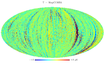
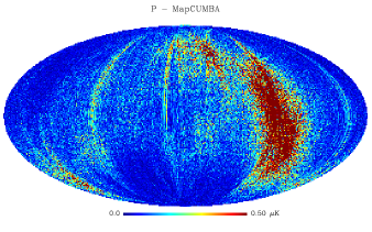
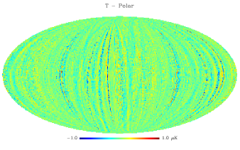
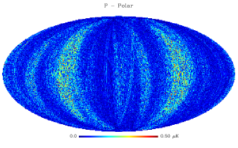
Figure 12: The difference maps between the noiseless output maps and the binned noiseless maps for MapCUMBA (top row) and Polar (bottom row). The maps contain CMB, dipole and foreground (CDF) and their resolution is $N_{\rm side}=512$. They are displayed here in ecliptic coordinates. The left hand maps are for the Stokes I and the right hand maps are for the magnitude $P$ of the polarisation vector ($P=\sqrt{Q^{2}+U^{2}}$). The map units are CMB microkelvins. (See www.helsinki.fi/~tfo_cosm/tfo_planck.html for better-quality figures.)

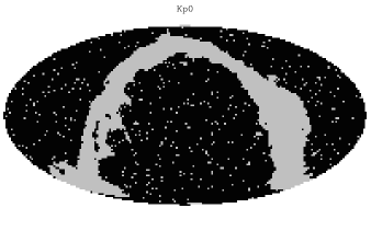
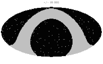
Figure 13: Masks showing two different schemes for removing the galaxy and $\sim$2000 strongest extra-galactic point sources from our maps. The light areas were removed. The left hand mask is the WMAP Kp0 mask (Bennett et al. bennett03b (2003)) after we had removed our point sources from it. We call this mask the Kp0 cut. The right hand mask removes our point sources and a region, that is 20$\degr$ above and below the galactic plane. We call this mask the $\pm$20$\degr$ cut. Note that the original WMAP Kp0 mask removes the point sources identified by the WMAP project. We did not have the WMAP point sources in our simulations, but we inserted our point sources randomly (see Sect. 3.5.2). Therefore our Kp0 cut removes more point sources than the $\pm$20$\degr$ cut. The sky coverage fractions of the masks are 0.758 (Kp0 cut) and 0.649 ($\pm$20$\degr$ cut). (See www.helsinki.fi/~tfo_cosm/tfo_planck.html for better-quality figures.)

5 Conclusions

We compared the output maps of three GLS map-making codes (MapCUMBA, MADmap, and ROMA) and three destriping codes (Polar, Springtide, and Madam). We made maps from simulated observations of four LFI 30 GHz detectors of the Planck satellite. The observed signal was comprised of dipole, CMB, diffuse galactic emissions, extragalactic radio sources, and detector noise. CMB, galactic and radio source signals included both total intensity (temperature) and polarisation. We assumed identical circularly symmetric beams for every detector. The GLS codes and Madam require information on the detector noise. Polar and Springtide do not rely on that information. In this study we assumed that the detector noise spectra were perfectly known.

We subtracted the binned noiseless map from the output maps of the map-making codes and examined the remaining residual map. It is a sum of two components: residual noise (due to detector noise) and signal error that arises from the subpixel signal structure that couples to the output map through the map-making.

The maps of the GLS codes have nearly the same residual noise levels, which are lower than the noise of the Polar and Springtide maps. Madam can produce maps with as low noise as the GLS codes. The residual noise of Springtide is higher than the noise of Polar, because Springtide works with long (1 hr) ring baselines rather than with shorter baselines used in Polar (1 min). These differences in the residual noise between the codes are, however, small.

The signal error was smallest in the Springtide maps, but the signal error of Polar was just a bit larger. The signal errors of the GLS codes were more significant. The signal error in the Madam maps was slightly smaller than in the GLS maps. However, the signal errors of all map-making codes were significantly smaller than their residual $1/f$ noise.

We examined several schemes to reduce the signal error. In destriping the most effective method was the reduction of the pixel size of the crossing points. For example, for $N_{\rm side}=512$ output maps we could reduce the rms of the signal error by a factor $\backsim$2 by using $N_{\rm side}=1024$ pixels (instead of $N_{\rm side}=512$ pixels) for the crossing points. We did not find methods to bring similar improvement in the GLS signal error. Reducing the crossing point pixel size in destriping increases the map noise slightly.

The next step in the map-making studies of the Planck CTP working group is to change to asymmetric beams and assume integration over non-zero sample intervals as detectors scan across the sky. This work has started and we will make maps from the simulated LFI 30 GHz observations using elliptic Gaussian beams that are fits to the realistic beam simulations. We will examine e.g. the quality of the maps and the magnitude of the leakage from temperature to polarisation due to differences between the responses of the detector beams.

- (1) Ashdown, M. 2006, submitted to A&A, [astro-ph/0606348]
- (2) Baccigalupi C., 2003, New Astron. Rev., 47, 1127
- (3) Bennett C.L. et al., 2003, ApJS, 148, 97
- Benoît et al. (2003) Benoît, A., Ade, P., Amblard, A. et al. 2003, A&A, 399, L19
- (5) Benoît A. et al., 2004, A&A, 424, 571
- Carretti et al. (2005) Carretti E., Bernardi G., Sault R.J., Cortiglioni S., Poppi S., 2005, MNRAS, 358, 1
- (7) Challinor, A., Fosalba, P., Mortlock, D., et al. 2000, Phys.Rev.D, 62, 123002
- (8) Doré, O., Teyssier, R., Bouchet, F.R., Vibert, D. & Prunet, S., 2001, A&A, 374, 358; see also http://ulysse.iap.fr/cmbsoft/mapcumba/
- (9) Duncan, A.R., Reich, P., Reich, W., Fürst, E. 1999, A&A, 350, 447
- (10) Dupac, X., & Tauber, J. 2005, A&A, 430, 363
- (11) Efstathiou, G., Lawrence, C., Tauber, J. et al. 2005, ”Planck - The Scientific Programme”, ESA-SCI(2005)1, ”Planck Bluebook” available in http://www.rssd.esa.int/Planck.
- Finkbeiner et al. (1999) Finkbeiner D.P., Davis M., Schlegel D.J. 1999, ApJ, 524, 867
- Giardino et al. (2002) Giardino G. et al., 2002, A&A, 387, 82
- (14) Górski, K.M., Hivon, E., & Wandelt, B.D. 1999, in Proceedings of the MPA/ESO Cosmology Conference ”Evolution of Large-Scale Structure”, ed. A.J. Banday, R.S. Sheth, & L. Da Costa, PrintPartners Ipskamp, NL, 37, [astro-ph/9812350]
- (15) Górski, K.M., Hivon, E., Banday, A.J., et al. 2005, ApJ, 622, 759
- (16) Górski, K.M., Wandelt, B.D., Hivon, E., Hansen, F.K., & Banday, A.J. 2005, ”The HEALPix Primer” (Version 2.00), available in http://healpix.jpl.nasa.gov
- Haslam et al. (1982) Haslam C.G.T., Stoffel H., Salter C.J., Wilson W.E., 1982, A&AS, 47, 1
- (18) Hivon, E. et al. 2006, under preparation
- (19) Jarosik, N. et al. 2006, submitted
- (20) Larquère, L. 2006, Ph.D. Thesis, Universite Paris 7 Denis-Diderot
- (21) O’Dwyer, I.J. et al. 2004, ApJ, 617, L99
- (22) Poutanen, T., de Gasperis, G., Hivon, E., et al. 2006, A&A, 449, 1311
- Prunet et al. (1998) Prunet S., Sethi S.K., Bouchet F.R., Miville-Deschenes M.A., 1998, A&A, 339, 187
- Reich & Reich (1986) Reich, P. & Reich, W. 1986, A&A Suppl, 63, 205
- (25) Reinecke, M., Dolag, K., Hell, R., Bartelmann, M., & Enßlin, T. 2006, A&A, 445, 373
- Tucci et al. (2002) Tucci M., et al., 2002, ApJ, 579, 607
- Tucci et al. (2004) Tucci M., Martinez-Gonzalez E., Toffolatti L., Gonzalez-Nuevo J., De Zotti G., 2004, MNRAS, 349, 1267
- Uyaniker et al. (1999) Uyaniker B., Frst E., Reich W., Reich P., Wielebinski R., 1999, A&AS, 138, 31
- (29) Wandelt, B. D., & Górski, K. M. 2001, Phys.Rev.D, 63, 123002