The presence of intermediate-mass black holes in globular clusters and their connection with extreme horizontal branch stars

Abstract

By means of a multimass isotropic and spherical model including self-consistently a central intermediate-mass black hole (IMBH), the influence of this object on the morphological and physical properties of globular clusters is investigated in this paper. Confirming recent numerical studies, it is found that a cluster (with mass $M$) hosting an IMBH (with mass $M_{\bullet}$) shows, outside the black hole gravitational influence region, a core-like profile resembling a King profile with concentration $c<2$, though with a slightly steeper behaviour in the core region. In particular, the core logarithmic slope is $s\la 0.25$ for reasonably low IMBH masses ($M_{\bullet}\la 10^{-2}M$), while $c$ decreases monotonically with $M_{\bullet}$. Completely power-law density profiles (similar to, e.g., that of collapsed clusters) are admitted only in the presence of a black hole with an unrealistic $M_{\bullet}>M$. The mass range estimate $12s-4.8<\log(M_{\bullet}/M)<-1.1c-0.69$, depending on the morphological parameters, is deduced considering a wide grid of models. Applying this estimate to a set of 39 globular clusters, it is found that NGC 2808, NGC 6388, M80, M13, M62, M54 and G1 (in M31) probably host an IMBH. For them, the scaling laws $M_{\bullet}\sim 0.09(M/\,\mathrm{M}_{\odot})^{0.7}\,\mathrm{M}_{\odot}$ and $M_{\bullet}\sim 50(\sigma_{\mathrm{obs}}/\textrm{km s}^{-1})^{1.2}\,\mathrm{M}_{\odot}$, are identified from weighted least-squares fit. An important result of this ‘collective’ study is that a strong correlation exists between the presence of an extreme blue horizontal branch (HB) and the presence of an IMBH. In particular, the presence of a central IMBH in M13 and NGC 6388 could explain why these clusters possess extreme HB stars, contrarily to the ‘second parameter counterparts’ M3 and 47 Tuc.

1 Introduction

The presence and origin of intermediate-mass black holes (IMBHs) at the centre of globular clusters, are still being debated inside the astrophysical community (see the recent general reviews in van der Marel, 2004; Rasio et al., 2006). There are essentially two main formation theories: they could be Population III stellar remnants (see, e.g., Madau & Rees, 2001) or could form in a runaway merging of young stars in sufficiently dense clusters (e.g., Portegies Zwart et al. 2004; Gürkan, Freitag, & Rasio 2004; Freitag, Gürkan & Rasio 2006b).

The IMBHs existence is suggested primarily by an argument of plausibility: they would fill the ‘embarrassing’ gap between stellar black holes (BHs; with mass $M_{\bullet}\la 10\,\mathrm{M}_{\odot}$) and super-massive BHs (having $M_{\bullet}\sim 10^{5}$–$10^{9}\,\mathrm{M}_{\odot}$) that are believed to reside in the nucleus of most galaxies (e.g., Kormendy, 2004; Richstone, 2004; Ferrarese & Ford, 2005, for recent reviews). By exploiting the accurate kinematical measurements of gas and stars in nearby galaxies, important correlations between the mass of super-massive BHs and various global properties of their hosting galaxy have been deduced (see Ferrarese & Ford, 2005, and references therein). For instance, extrapolating the Magorrian et al. (1998) relation – $M_{\bullet}\sim 10^{-3}$ times the mass of the host system – to globular clusters, these would contain BHs with an intermediate mass $M_{\bullet}\sim 10^{2}$–$10^{4}$. Indirect observational evidences come from the detection of ultra-luminous X-ray sources radiating at super-Eddington luminosity ($>10^{39}$ erg s^-1) and thought to originate from matter infall on BHs considerably more massive than stellar BHs (see Fabbiano, 2006, for a review on this subject).

In globular clusters, however, direct kinematic observations are seriously obstacled by crowding and by the relatively small number of stars inside the BH gravitational influence region (hereafter BHIR), which cannot be well resolved in many cases. Thus, so far, only very few clusters have been the object of accurate kinematic studies so as to infer about the possible presence of massive objects in the central regions.

We just remind the cases of the core-collapsed clusters M15 (Gerssen et al. 2002, 2003; McNamara, Harrison & Anderson 2003) and 47 Tuc, in which such a presence is not confirmed yet by the latest observational data (van den Bosch et al. 2006 and McLaughlin et al. 2006, respectively), and the highly concentrated and massive cluster G1 (in M31), where a central $\sim 2\times 10^{4}\,\mathrm{M}_{\odot}$ IMBH has been claimed to reside (Gebhardt, Rich, & Ho, 2002, 2005), while a recent deep photometric analysis of the core region of $\omega$ Cen seems to be consistent with an IMBH with mass $\sim 10^{4}\,\mathrm{M}_{\odot}$ (Noyola, Gebhardt & Bergmann, 2006). Note, however, that for both M15 and G1, direct and accurate $N$-body simulations reproduce the observed mass-to-light ratio without the need of an IMBH (Baumgardt et al., 2003a, b), although the peculiar scenario of a two clusters merging event is required in the case of G1.

Other, less direct, insights can be gained from the time behaviour of the period of millisecond pulsars sited in clusters central region, which permits to deduce the local acceleration. This occurs in the intriguing case of NGC 6752 where there are indications of the existence of an underluminous and compact component with mass $\sim 10^{3}\,\mathrm{M}_{\odot}$ (Ferraro et al., 2003; Colpi et al., 2005, and references therein).

It is interesting to note that the above-mentioned individual studies concerned globular clusters that are supposed to host IMBH because of their (present) high central density and (presently) high rate of stellar collisions in their compact cores. Nevertheless, present conditions may be drastically different from those at the early epochs of clusters life. More importantly, as firstly argued by Baumgardt, Makino, & Hut (2005), their dynamical status could be even inconsistent with the long-term effects that a IMBH actually produces on the cluster internal evolution. Using collisional $N$-body simulations, Baumgardt et al. found that the high stellar density in the vicinity of the central IMBH enhances the rate of close encounters that, in turn, induces a rapid expansion of the central region, giving rise to a medium-concentration, King-like profile, whose features are almost independent of the BH mass. They argued that an observable fingerprint of the IMBH presence is just a slight slope of the density in the core region, thus suggesting as probable candidate clusters hosting IMBH, those having a surface brightness logarithmic slope $\sim-0.2$ in the core (while the typical projected profile of core-collapsed systems goes like $r^{-1}$).

Similar conclusions have been recently reached by Trenti et al. (2007) who conducted direct $N$-body experiments of clusters with IMBHs and realistic fractions of primordial binaries: the expansion of the core is further enhanced and the formation of the density cusp is confined in the immediate vicinity of the BH. This leads to density profiles with a core to half-mass radius ratio significantly higher than when the IMBH is absent (Trenti, 2006). All these studies are telling us that a IMBH represents a ‘heat’ source in the central region, acting in a way similar to hardening binaries in contrasting gravothermal collapse (see also Heggie & Hut, 2003).

However, besides these global morphological hints, other fingerprints of the IMBH presence could be revealed. As known, one of the most important effect of the gravitational influence of the IMBH on the surrounding stars, is the tidal erosion and disruption they undergo during close passages (see, e.g., Frank & Rees 1976; Amaro-Seoane, Freitag & Spurzem 2004; Baumgardt, Makino, & Ebisuzaki 2004a; Freitag, Amaro-Seoane & Kalogera 2006a; Baumgardt et al. 2006). Besides complete disaggregation, this may lead to a loss of envelope mass of passing-by giants. The mass loss from stellar outer layers is also one of the possible explanation for the not yet ascertained origin of ‘blue subdwarfs’ – also called extreme horizontal branch stars, see Rich et al. 1997 and, for a review on this subject in the context of dense galactic nuclei, also Alexander 2005, section 3.4. These are stars heavier and bluer than turn-off stars, and they are located at the lower-left end of the horizontal branch (HB), in the region of the color-magnitude diagram referred to as extreme HB (hereafter EHB; see the discussion in Meylan & Heggie 1997, sect. 9.7, and the recent review in Catelan 2007).

Given the cuspy behaviour of the stellar density in the BHIR and the relatively high ratio between $M_{\bullet}$ and the single stellar mass, it is reasonable to expect that the above-mentioned mechanism of blue subdwarfs formation is significantly enhanced by the presence of the IMBH. Thus, the possibility to find some connection between this presence and that of an abundant population of EHB stars naturally emerges and, to our knowledge, has never been explored so far. This is one of the aim of the present paper.

While the direct investigation of the dynamical evolution of a cluster harbouring a massive compact object is still at the beginning – because of the recent development of sufficiently advanced computational tools – the study of the stellar phase-space distribution function (DF) around a massive BH in the quasi-steady regime is a classical subject in Stellar Dynamics tackled by several authors since the early 70s (Peebles, 1972; Bahcall & Wolf, 1976; Shapiro & Lightman, 1976; Lightman & Shapiro, 1977; Cohn & Kulsrud, 1978). If a time much longer than the cluster relaxation time is passed since the BH formation and accretion, dynamical and ‘thermal’ equilibrium can take place and a Maxwellian DF $\sim\exp(-E/\sigma^{2})$, with $E$ the total energy and $\sigma$ a velocity parameter, should be established. Nevertheless, close enough to the compact object, stars are either disrupted, because of the strong tidal interaction, or swallowed by the BH, thus generating an outward flux of positive energy that, in stationary conditions, must be constant and uniform through the central region. This precludes the Maxwellian distribution being valid in the BH vicinity. Simple scaling arguments (Binney & Tremaine, 1987, section 8.4.7) or treatments based on the ‘heat-transfer’ equation (Freitag et al., 2006b, section 2.2) show, indeed, that a realistic space density behaviour is $\sim r^{-7/4}$.

Such a power-law density (or ‘cusp’) corresponds to a DF $\sim(-E)^{1/4}$, as was first found, through approximate solutions of the Fokker-Planck equation, by Bahcall & Wolf (1976) (hereafter BW76, ) and more recently confirmed with the help of more accurate methods including relaxation effects, such as: Monte-Carlo codes (Shapiro, 1985; Freitag & Benz, 2002), gas-dynamical methods (Amaro-Seoane et al., 2004) and direct $N$-body simulations (Baumgardt et al. 2004a; Preto, Merritt & Spurzem 2004).

However, equilibrium self-consistent models of stellar systems including massive BHs are not so numerous. We just mention the Gerssen et al. (2002) paper on M15 employing spherical non-parametric models and the papers by van den Bosch et al. (2006) and van de Ven et al. (2006), in which axisymmetric models of, respectively, M15 and $\omega$ Cen are generated to infer the radial behaviour of the $M/L$ ratio, by means of a generalization of the Schwarzschild (1979) orbit superposition method. A further generalization of this technique has been also recently presented in Capuzzo Dolcetta et al. (2007) to model triaxial galaxies with dark matter and a central density cusp. It is worth noting, finally, that McLaughlin et al. (2006), in order to derive hints about the presence of an IMBH in 47 Tuc, applied a single-mass and isotropic King model, even if in a not fully self-consistent way.

In the present study, a self-consistent parametric model is constructed and used to estimate the mass of possible IMBHs in clusters and their influence on the cluster density profile, as well as on the presence of EHB stars. It basically consists of a multimass King model appropriately extended to incorporate the BW76 DF inside the BHIR. The model is spherical, isotropic (in the present version) and relatively easy to construct and use. Its multimass nature makes straightforward the inclusion of central energy equipartition, which is suggested to play a non-negligible role in the presence of a massive BH, too (Bahcall & Wolf 1977; Murphy, Cohn, & Durisen 1991; Baumgardt, Makino, & Ebisuzaki 2004b; Freitag et al. 2006b; Hopman & Alexander 2006).

The model will be described in section 2, while in section 3 the observable features of the generated surface brightness and velocity dispersion profiles will be illustrated, also with respect to the debated structural properties of clusters hosting IMBH. Then, in section 4, the model will be employed to deduce the mass of possible IMBHs from the central density profiles provided by the recent Noyola & Gebhardt (2006) (hereafter NG06, ) analysis of WFPC2 Hubble Space Telescope (HST) observations of 38 galactic globulars (G1 in M31 is considered as well). In section 5, finally, the connection between the existence of IMBHs and the presence of EHBs will be investigated. Conclusions will be drawn in section 6.

2 Description of the parametric model

In the following, given the length-, velocity- and density-scale parameters, $\tilde{r}$, $\sigma$ and $\tilde{\rho}$, respectively, it is convenient to deal with dimensionless quantities, namely:

radius $x\equiv r/\tilde{r}$;

velocity $w\equiv v/\sigma$;

mean total potential $W(x)\equiv-\Psi(x)/\sigma^{2}$;

energy (per unit mass) $E\equiv w^{2}/2-W$;

density $\nu(x)\equiv\rho(x)/\tilde{\rho}$;

cluster mass in stars inside the radius $x$, ${\cal M}(x)\equiv M(x)/\tilde{\rho}\tilde{r}^{3}$.

BH mass $\mu\equiv M_{\bullet}/\tilde{\rho}\tilde{r}^{3}$.

A suitable DF can be given by generalizing the King (1966) lowered Maxwellian, so as to include the BW76 DF below a proper ‘transition’ energy, i.e.

$$f(E)=\left\{\begin{array}[]{ll}c(-E)^{1/4},&\textrm{if $E<-W_{\mathrm{BH}}$,}\\ (2\pi)^{-3/2}(\mathrm{e}^{-E}-1),&\textrm{if $-W_{\mathrm{BH}}\leq E<0$,}\\ 0,&\textrm{if $E\geq 0$,}\end{array}\right.$$ (1)

where the coefficient $c\equiv(2\pi)^{-3/2}(\mathrm{e}^{W_{\mathrm{BH}}}-1)W_{\mathrm{BH}}^{-1/4}$ assures the $f$ continuity and $W$ is defined so to have $W(x_{\mathrm{t}})=0$ where $x_{\mathrm{t}}$ is the model ‘limiting radius’. The ‘transition’ potential $W_{\mathrm{BH}}\equiv W(x_{\mathrm{BH}})$ is considered to be the potential on the surface of the sphere, with radius $x_{\mathrm{BH}}$, coinciding with the BHIR.

The BHIR can be defined as the largest sphere, centered at the BH position, in which the motion of the stars is dominated by the field generated by the compact object. This definition is coherent with the assumption of Maxwellian behaviour just outside this region (i.e., for $E\geq-W_{\mathrm{BH}}$). Then, a reasonable condition for $x_{\mathrm{BH}}$ is that the enclosed mass in stars is a small fraction of the BH mass, i.e.

$${\cal M}(x_{\mathrm{BH}})=0.1\mu,$$ (2)

even if this forces to solve (as we will see later) an implicit equation that involves a mass profile that is only a-posteriori known. This condition is similar to that adopted in Merritt (2004); nevertheless we chose a smaller fraction ($0.1$ instead of $2$) to ensure the validity of the power-law behaviour for $f(E)$ (see BW76, section IIIc).

The usually adopted formula $x_{\mathrm{BH}}\sim GM_{\bullet}/\langle v^{2}\rangle\tilde{r}$ (BW76; Baumgardt et al. 2004a, b) is not a-priori compatible with this BHIR definition, because it gives a radius that yields typically ${\cal M}(x_{\mathrm{BH}})\la 10^{-4}\mu$. Indeed, even if the BHIR has to be sufficiently small for the BH gravitational field to dominate the dynamics inside, on the other hand it must be large enough to make plausible the hypothesis of isothermal distribution outside it. This latter condition would not be realistic in an environment in which the BH still exerts a strong influence on the dynamics (BW76).

The DF of equation (1) guarantees the ‘dynamical equilibrium’ of the system, in the sense that, according to the Jeans theorem, it is a solution of the collisionless Boltzmann equation. The presence of a massive BH, assumed to be located at rest in the cluster centre, makes that the potential time-independence is preserved and thus the DF of equation (1) is still a valid equilibrium solution, because $E$ remains an integral of motion. Therefore, one can proceed in the same manner as in obtaining usual King models, that is – as required by the self-consistency – just by solving, for $W(x)$, the dimensionless Poisson’s equation in spherical symmetry

$$\frac{d^{2}W}{dx^{2}}+\frac{2}{x}\frac{dW}{dx}=-(4\pi G\tilde{\rho}\tilde{r}^{2}\sigma^{-2})\nu(W),\textrm{ for }x>0,$$ (3)

where the origin is excluded to avoid the BH singularity and the stellar density, expressed as a function of $W$, is

$$\nu(W)=\ \ 4\pi\int_{0}^{\sqrt{2W}}f(E)w^{2}\mathrm{d}w=\left\{\begin{array}[]{ll}\nu_{1},&\textrm{if $W\leq W_{\mathrm{BH}}$,}\\ \nu_{2},&\textrm{if $W>W_{\mathrm{BH}}$,}\end{array}\right.$$ (4)

where

$$\nu_{1}(W)\equiv\mathrm{e}^{W}\mathrm{erf}\left(\surd W\right)-\frac{2}{\sqrt{\pi}}\left(W^{1/2}+\frac{2}{3}W^{3/2}\right)$$ (5)

and

$$\nu_{2}(W)\equiv 4\pi c\int_{\sqrt{2W_{\mathrm{BH}}}}^{\sqrt{2W}}\left(W-\frac{w^{2}}{2}\right)^{1/4}w^{2}\mathrm{d}w\,+$$

$$\ \ \nu_{1}(W_{\mathrm{BH}})=2^{7/2}\pi cg(W)W^{7/4}+\nu_{1}(W_{\mathrm{BH}}).$$ (6)

The first term of the r.h.s. of equation (6) is the density corresponding to a polytropic stellar model with index $=7/4$ (Binney & Tremaine, 1987), with

$$g(W)=\int_{0}^{\,\theta}\left(\sin^{3/2}y-\sin^{7/2}y\right)\mathrm{d}y,$$ (7)

where $\theta\equiv\cos^{-1}\sqrt{W_{\mathrm{BH}}/W}$, $0\leq\theta\leq\pi/2$.

The integral in equation (7) yields

$$g(W)=-\frac{4}{21}\left[F\left(\frac{\pi}{4}-\frac{\theta}{2}\right)-F\left(\frac{\pi}{4}\right)\right]-$$

$$\ \ \frac{1}{42}(5\cos\theta+3\cos 3\theta)\surd\sin\theta=$$

$$\ \ -\frac{4}{21}\left[F\left(\frac{\pi}{4}-\frac{\theta}{2}\right)-F\left(\frac{\pi}{4}\right)+(3\omega-1)(1-\omega)^{1/4}\frac{\surd\omega}{2}\right],$$ (8)

where $\omega\equiv W_{\mathrm{BH}}/W$ and $F(\phi)\equiv\int_{0}^{\phi}(1-2\sin^{2}y)^{-1/2}\mathrm{d}y$ is an elliptic integral of the first kind that can be accurately evaluated by standard numerical iterative procedures (see, e.g., Press et al., 1988, sect. 6.11).

As in standard King models, it is convenient to impose the relation

$$\tilde{r}^{2}=\frac{9\sigma^{2}}{4\pi G\tilde{\rho}}.$$ (9)

With this choice equation (3) becomes

$$\frac{d^{2}W}{dx^{2}}+\frac{2}{x}\frac{dW}{dx}=-9\nu(W),\textrm{ for }x>0,$$ (10)

that has a family of solutions depending only on the boundary conditions (with $x_{0}>0$),

$$\begin{array}[]{lcl}\frac{dW}{dx}(x_{0})&=&W^{\prime}_{0},\\ W(x_{0})&=&W_{0}.\end{array}$$ (11)

Choosing $x_{0}=x_{\mathrm{BH}}$, these conditions define a two-parameters $(W_{\mathrm{BH}}^{\prime},W_{\mathrm{BH}})$ set of models, with all the others being just scaling parameters.

By the definition of BHIR it can be assumed that

$$\frac{d\Psi}{dr}(x_{\mathrm{BH}})=\frac{GM_{\bullet}}{(x_{\mathrm{BH}}\tilde{r})^{2}}=\frac{G\mu}{x_{\mathrm{BH}}^{2}}\tilde{\rho}\tilde{r},$$ (12)

that, using equation (9), leads to

$$W_{\mathrm{BH}}^{\prime}=-\frac{9\mu}{4\pi x_{\mathrm{BH}}^{2}}.$$ (13)

Thus, the whole set of models can be conveniently described by the pair $(\mu,W_{\mathrm{BH}})$, while the solution inside the BHIR can be found by integrating equation (3) backwards from $x_{\mathrm{BH}}$ to a given minimum radius, which we generally set equal to $0.1x_{\mathrm{BH}}$.

Finally, $x_{\mathrm{BH}}$ must be a solution of equation (2) with ${\cal M}(x)$ given self-consistently by the model that uses $x_{\mathrm{BH}}$ itself as a BHIR radius. This is found iteratively, evaluating the ‘new’ radius $x_{\mathrm{BH}}^{\mathrm{new}}$ through equation (2) with ${\cal M}(x)$ generated employing the previous value of $x_{\mathrm{BH}}$. The process starts with an initial guessed $x_{\mathrm{BH}}=GM_{\bullet}/3\sigma^{2}\tilde{r}$ and is halted when the difference between two subsequent values stays within a given tolerance (we chose $|x_{\mathrm{BH}}^{\mathrm{new}}-x_{\mathrm{BH}}|/x_{\mathrm{BH}}<0.1$).

2.1 Inclusion of a mass spectrum

The continuum stellar mass spectrum of the real cluster can be represented by a set of $n$ stellar components, each one having a star mass $m_{k}$, a total mass $M_{k}$ and a velocity parameter $\sigma_{k}$. The DF of the more realistic multimass case, $f_{\mathrm{mm}}$, can be given as a linear combination of the $f$ of equation (1) (see, e.g., Da Costa & Freeman, 1976; Gunn & Griffin, 1979):

$$f_{\mathrm{mm}}(E)=\sum_{k=1}^{n}\alpha_{k}f_{k}(E)=\sum_{k=1}^{n}\alpha_{k}f(\beta_{k}E),$$ (14)

where $\alpha_{k}$ serve to reproduce the given mass function and $\beta_{k}\equiv\sigma^{2}/\sigma^{2}_{k}$.

A more rigorous treatment would require $f_{k}$ to explicitly depend on $m_{k}$ through the exponent of $E$ in the DF inside the BHIR, as a consequence of mass segregation. This dependence was quantified by Bahcall & Wolf (1977) and then confirmed (at least partially) by means of Fokker-Planck (Murphy et al., 1991), $N$-body (Baumgardt et al., 2004b) and Monte-Carlo (Freitag et al., 2006a) simulations. Nevertheless, the small gain in ‘theoretical coherence’ might be vanified by the use of a discrete set of stellar masses instead of the real continuous mass spectrum. Furthermore, the model would be complicated by the need of separate numerical quadratures in equation (4) for each mass class. For these reasons, we simplified the model construction by considering the same $1/4$ energy exponent in $f(E<-W_{\mathrm{BH}})$, regardless of the stellar mass. However, the energy equipartition, responsible of mass segregation, can be still reproduced at the border of the BHIR by a suitable choice of $\beta_{k}$ (see below).

Thus, the multicomponent Poisson equation has the same form of equation (10) apart from $\nu$ that is replaced by the total density

$$\nu_{\mathrm{tot}}(W)\equiv\sum_{k=1}^{n}\frac{\alpha_{k}}{\beta_{k}^{\,3/2}}\nu(\beta_{k}W),$$ (15)

where $\nu$ is given here by equation (4).

Once a component is arbitrarily chosen as the ‘reference’ one, say the first one, without loss of generality one can assume $\sigma=\sigma_{1}$, i.e. $\beta_{1}=1$. Then, since the set of $\alpha_{k}$ are constrained by the given set of $M_{k}$, the solutions of the Poisson equation are determined just by the boundary conditions (11) at $x_{0}=x_{\mathrm{BH}}$. Indeed, the set of $\beta_{k>1}$ can be fixed by the requirement of energy equipartition in the central region. To do that, the procedure described in Miocchi (2006) is applied at the radius $x_{\mathrm{BH}}$. In practice, once given $\sigma$ and $W_{\mathrm{BH}}$, we have

$$\beta_{k}=W_{\mathrm{BH}}^{-1}\kappa^{-1}\left[\frac{m_{1}}{m_{k}}\kappa(W_{\mathrm{BH}})\right],$$ (16)

with $\kappa$ the function defined in equation (8) of Miocchi (2006), and $\sigma^{2}_{k}=\sigma^{2}/\beta_{k}$.

Thus, $W_{\mathrm{BH}}$ and $\mu$ determine a 2-parameters family of models [through equation (13)] also in the multimass case. Note, furthermore, that $f_{k}$ does now depend on $m_{k}$, through $\beta_{k}$.

As regards $x_{\mathrm{BH}}$, the same iterative procedure described in the single-component case is employed to find the value that solves equation (2). Finally, as a consistency test, the velocity dispersion profile generated by the model is compared with that deduced by the spherical isotropic Jeans’ equation (Binney & Tremaine, 1987),

$$\langle w^{2}\rangle_{J}(x)=\frac{27}{4\pi\nu_{\mathrm{tot}}(x)}\int_{x}^{x_{\mathrm{t}}}\nu_{\mathrm{tot}}(y)[{\cal M}(y)+\mu]y^{-2}\mathrm{d}y,$$ (17)

and the model output $[{\cal M}(x),\nu_{\mathrm{tot}}(x)]$ is accepted only if the difference between the two profiles (evaluated as a $\chi^{2}$ summation over the spatial grid points) is small enough (e.g., to within 90 percent of confidence level).

3 Surface brightness profiles with IMBH

To understand how the presence of an IMBH influences the shape of a typical projected profile, it is instructive to examine the results of a single-mass model first. In Fig.s 1 and 2, various projected surface density profiles ($\Sigma$) are plotted, fixing $W_{\mathrm{BH}}=9.5$, for some of the models written on Table 1. As a comparison, a standard King model is also plotted with $W_{0}=9.5$.

Table 1: Relevant parameters for single-mass models generated with $W_{\mathrm{BH}}=9.5$. Some of them are plotted in Fig.s 1 and 2. $\mu$ is the dimensionless BH mass, $M_{\bullet}/M$ is the BH mass in units of total cluster mass, $c$ is the concentration defined according to Equation (18), $x_{\mathrm{BH}}$ is the BHIR radius, $x_{\mathrm{cu}}$ is the cusp radius, $x_{\mathrm{c}}$ is the core radius and $s$ is the logarithmic slope of the projected surface density around $x_{\mathrm{cu}}$. In the last line $x_{\mathrm{cu}}>x_{\mathrm{t}}$ (i.e. $c<0$) indicates the presence of a full cuspy profile (in this case $x_{\mathrm{c}}$ is a meaningless quantity).

$\mu$	$M_{\bullet}/M$	$c$	$x_{\mathrm{BH}}$	$x_{\mathrm{cu}}$	$x_{\mathrm{c}}$	$s$
no BH	$0$	$2.2$	$0$	$0$	$0.92$	$0$
$0.05$	$5.9\times 10^{-4}$	$2.2$	$0.10$	$0.18$	$1.0$	$7.4\times 10^{-2}$
$0.2$	$2.4\times 10^{-3}$	$2.1$	$0.15$	$0.30$	$1.2$	$0.18$
$0.5$	$6.0\times 10^{-3}$	$1.8$	$0.16$	$0.56$	$2.2$	$0.25$
$0.8$	$8.4\times 10^{-3}$	$1.4$	$0.16$	$1.1$	$4.6$	$0.19$
$1$	$8.9\times 10^{-3}$	$1.1$	$0.15$	$1.9$	$8.5$	$0.14$
$1.4$	$9.0\times 10^{-3}$	$0.87$	$0.14$	$6.0$	$28$	$9.8\times 10^{-2}$
$1.5$	$9.3\times 10^{-3}$	$0.80$	$0.14$	$8.8$	$42$	$8.8\times 10^{-2}$
$1.6$	$1.0\times 10^{-2}$	$0.78$	$0.14$	$14$	$66$	$7.7\times 10^{-2}$
$1.8$	$1.8\times 10^{-2}$	$0.77$	$0.14$	$84$	$330$	$0.12$
$2$	$9.2$	$<0$	$0.14$	$>x_{\mathrm{t}}$		$>1$

As expected, we can see that the BH gives rise to a cuspy behaviour extended from the centre up to a radius that can be called the ‘cusp’ radius, $x_{\mathrm{cu}}$, above which the much flatter core region begins. An ‘operative definition’ of this radius can be given as the radius where the surface brightness profile shows a concavity change (while $x_{\mathrm{cu}}\equiv 0$ if the inflection point is not evident, i.e. if the cusp is not observed). However, this radius was found to be well approximated – at least in the range of BH masses studied here ($M_{\bullet}/M\la 2$ per cent) – by the radius containing half the BH mass in stars [${\cal M}(x_{\mathrm{cu}})=\mu/2$].

Moreover, it is convenient to define the ‘core’ radius $x_{\mathrm{c}}$ as equal to the radius at which the surface brightness drops to $1/2$ the value at $x_{\mathrm{cu}}$. Indeed, it is important to adopt a concentration parameter that is unambiguously defined when a density cusp is present. In particular, the parameter

$$c\equiv\log\left(\frac{x_{\mathrm{t}}}{x_{\mathrm{c}}}\right)$$ (18)

is preferable to the standard King concentration parameter $c_{\mathrm{K}}=\log(x_{\mathrm{t}})$, because this latter is based on the length-scale $\tilde{r}$ that has no immediate relation with any relevant morphological feature of our IMBH models. However, it has been checked that an IMBH model with a given $c$ yields a profile that is well matched, in the core and in the tidal region, by that of a standard King model with $c_{\mathrm{K}}=c$. Note, also, that in the profiles depicted in Fig.s 1 and 2, $x_{\mathrm{c}}$ corresponds to the location of the ‘knee’ of the curves, in analogy to a standard King profile. Thus, in clusters whose central luminosity cusp is not resolved, one can infer about the presence of an IMBH directly using the standard $c_{\mathrm{K}}$ parameter coming from observations.

From these profiles (plotted as a function of the radius measured in unit of $x_{\mathrm{c}}$) three relevant features can be immediately noticed:

1. the projected density in the core region is not as flat as in standard King model, (see inset in Fig.s 1b and 2b)

2. the presence of a central IMBH reduces significantly the concentration of the profile in comparison with a BH-free model with $W_{0}=W_{\mathrm{BH}}$, and

3. the concentration decreases for increasing $\mu$.

These features are confirmed (as we will see later) in the case of multimass models, too.

Figure 1: (a) Behaviour of the potential and (b) projected surface density profile (scaled so as to give $\Sigma=1$ at the cusp radius) for single-mass models with $W_{\mathrm{BH}}=9.5$ and with various IMBH mass as indicated ($\mu=0$ means a standard King model, with $W_{0}=9.5$). The dots mark the BHIR radii, while the arrows indicate the cusps radii ($x_{\mathrm{cu}}$). The panel (b) inset shows the profiles in the core region around $x_{\mathrm{cu}}$. The concentration parameters are also reported in panel (a).

Figure 2: The same as in Fig. 1 for models with higher BH mass. Since in this case the cusp radii are nearly equal, only one arrow is plotted.

The last two points can be easily understood from the behaviour of the potential (Fig.s 1a and 2a) that, at $x_{\mathrm{BH}}$, has a different slope when compared with the (practically flat) King model. The potential with the BH decreases below $W_{\mathrm{BH}}$, then becomes flatter in the core (before dropping in the tidal region) leading the system to a lower concentration profile in comparison with the BH-free case. This suggests that the presence of a IMBH induces profiles with a large core.

Note, from Table 1, the rapid growth of the cusp radius for $\mu>1$; for $\mu=2$, it becomes even larger than the limiting radius making, in fact, $\Sigma(x)$ to “jump” to a completely cuspy behaviour (not shown in the Figures), without any recognizable core. Since this leads to $M_{\bullet}>M$, such kind of configurations are discarded throughout our analysis, as unrealistic for globular clusters. Therefore – once the validity of the DF of equation (1) is accepted – reasonable values of the BH mass at the centre of GCs are compatible only with a core-like profile. The density cusp is confined in the very inner region of the core.

All this is in remarkable agreement with the results of Baumgardt et al. (2005) and Trenti et al. (2007), obtained by means of collisional $N$-body simulations including IMBH. These simulations have shown that the presence of an IMBH initially enhances the rate of exchange of energy in close encounters among stars moving in the cusp region; this gives rise to a strong cluster expansion which, in turn, yields final profiles well fitted by King models, with a relatively low concentration (see also Baumgardt et al., 2004a, b).

Finally, the apparent contradiction that can be seen in Fig.s 1–2 of a decreasing BHIR radius for increasing BH masses, is actually due to the scaling of the radius with $x_{\mathrm{c}}$ and to the fact that the core radius grows quite rapidly while $x_{\mathrm{BH}}$ is nearly constant (see Table 1). The decrease of the ratio $x_{\mathrm{BH}}/x_{\mathrm{c}}$ is a consequence of the lower and lower concentration that these models show for growing BH masses. Another consequence is the unexpected decrease of the logarithmic slope ($s$, with $\Sigma\sim x^{-s}$) of the surface density around $x_{\mathrm{cu}}$, that can be seen for $\mu>0.5$ (see Table 1 and Fig. 2b inset).

3.1 The multimass case

At this point, one could study in more detail the dependence on the BH mass of both $c$ and the slope of $\Sigma(x)$ in the core region. Nevertheless, it is more appropriate to make this analysis directly in the multimass context, which is (for globular clusters) a much more realistic scenario than that of the single-mass case, because the mass-segregation could heavily change the effect of the presence of the BH in the brightness profile (Baumgardt et al., 2005).

Thus, a stellar mass spectrum is included assuming a Salpeter mass function (${\mathrm{d}}N\propto m^{-1.35}\mathrm{d}\log m$) and considering $7$ mass bins in the range $0.25$ – $0.83\,\mathrm{M}_{\odot}$, along with light and heavy remnants, following the prescriptions of Côté et al. (1995). Nevertheless, their lightest mass class was not included because it is below the lower mass limit predicted, under energy equipartition, in Miocchi (2006). See Table 2 for the list of parameters for the adopted stellar components.

Table 2: Values for the components used in the multimass model. MS = main sequence stars; G = giants; HB = horizontal branch stars; WD = white dwarfs (from Côté et al., 1995).

$k$	mass range $(\,\mathrm{M}_{\odot})$	$M_{k}/M$	$m_{k}(\,\mathrm{M}_{\odot})$	$(L/M)_{k}$	$\sigma_{k}/\sigma$	content
$1$	$0.75$–$0.83$	$4.9\times 10^{-2}$	$0.79$	$10$	$1$	MS, G, HB
$2$	$4$–$8$	$3.9\times 10^{-2}$	$1.2$	$0$	$0.81$	WD
$3$	$0.65$–$0.75$	$0.18$	$0.70$	$0.19$	$1.1$	MS + WD
$4$	$0.55$–$0.65$	$9.3\times 10^{-2}$	$0.60$	$6.5\times 10^{-2}$	$1.2$	MS
$5$	$0.45$–$0.55$	$0.24$	$0.50$	$2.3\times 10^{-2}$	$1.3$	MS + WD
$6$	$0.35$–$0.45$	$0.16$	$0.39$	$1.0\times 10^{-2}$	$1.6$	MS
$7$	$0.25$–$0.35$	$0.24$	$0.29$	$4.9\times 10^{-3}$	$5.7$	MS

Figure 3: (a) Concentration parameter obtained for a grid of values of $M_{\bullet}/M$, and $W_{\mathrm{BH}}$; no realistic models can be generated above the dashed line. (b) Behaviour of $c$ as a function of BH mass for some values of $W_{\mathrm{BH}}$, as indicated.

Figure 4: As in Fig. 3 for the logarithmic slope of the surface brightness at the cusp radius.

The qualitative behaviours of the apparent concentration and of the $\Sigma$ slope as a function of the BH mass discussed in the single-component case, are basically confirmed by the curves plotted in Fig.s 3b–4b. They refer to a grid of models computed in the range $15\leq W_{\mathrm{BH}}\leq 9.5$ and $10^{-2}\leq\mu\leq 0.15$. In this case the concentration has been evaluated on the total projected surface brightness profile, $I(x)$, and the logarithmic slope $s$ is again such that $I\sim x^{-s}$. It is worth noting that:

1. $c$ decreases monotonically with the BH mass

2. according to our model, IMBHs with $M_{\bullet}\ga 10^{-3}M$ can exist only for non-collapsed distributions ($c\la 2$) exhibiting a logarithmic slope in the core which is $\la 0.25$ for reasonably low BH masses ($M_{\bullet}\la 10^{-2}M$)

3. $s$ increases for growing BH mass up to a maximum value, then the lower concentration achieved makes the core region to be much wider than the cusp region, causing the decrease of $s$.

These features fully confirm the Baumgardt et al. (2005) findings. In particular, the logarithmic slope is compatible with the range of values found for the clusters studied by these authors’ $N$-body simulations.

In Fig. 3b it is apparent a certain degree of self-similarity of the various curves; of course, lower concentrations can be in principle obtained starting from lower $W_{\mathrm{BH}}$ – though this imposes an even higher mass cut-off of the stellar mass function at the low-mass end in order to ensure energy equipartition. Thus, no lower limit on $c$ can be fixed. On the contrary, an upper limit to the concentration exists (roughly indicated by the dashed line in Fig. 3a). The same argument holds for $s$ (Fig. 4), for which lower values could be obtained for lower $W_{\mathrm{BH}}$. Therefore, combining the upper limits of the two quantities, a range of admitted values is found for the BH mass:

$$11.6s-4.85\la\log\left(\frac{M_{\bullet}}{M}\right)\la-1.14c-0.694.$$ (19)

3.1.1 The effect of mass segregation

The presence of mass segregation (as due to the imposed energy equipartition at $x_{\mathrm{BH}}$) is evident in Fig. 5. Three components are represented: the brightest component, the heavy remnants one and the lightest MS stars component ($k=1,2$ and $7$, respectively, in Table 2). The first component gives almost all the cluster luminosity. The model has been generated with $W_{\mathrm{BH}}=9.5$ and $\mu=0.155$, corresponding to $M_{\bullet}/M=6\times 10^{-3}$.

In the core region the lightest (heaviest) stars have the highest (lowest) velocity dispersion and, consequently, the least (most) concentrated density profile. The lightest star component is practically unaffected by the presence of the BH, while inside the BHIR the density cusp is particularly evident for the most massive stars.

We note that the space density of each component must have the same asymptotic BW76 behaviour $\sim x^{-\gamma}$, with $\gamma=7/4$ (i.e. $\sim W^{7/4}$), because it was assumed for simplicity that all the $f_{k}$ in equation (14) have the same functional form. Nevertheless, how much deep one has to go towards the centre to find the $x^{-7/4}$ cusp depends on $\beta_{k}$ and, in turn, on the component stellar mass. This is because the density of the $k$th component is a function of $\beta_{k}W\propto\sigma^{-2}_{k}$ [equation (15)]; thus, the higher the velocity dispersion of the stars is, the deeper the extent of the region where the ‘isothermal plateau’ prevails, and the flatter the density is at a fixed radius.

With this in mind, in Fig. 6 the log slope $\gamma$ of the space mass density in the cusp region is plotted as a function of the stellar mass. The slope is evaluated well inside the BHIR, namely at $\sim x_{\mathrm{BH}}/5$, i.e. where the enclosed mass in stars is of order $10^{-2}M_{\bullet}$. It can be noticed that sufficiently massive stars ($m\ga 0.6\,\mathrm{M}_{\odot}$) show a slope close to the linear relation $\gamma\simeq 1.8m/(0.8\,\mathrm{M}_{\odot})$, of the kind of that predicted by the multicomponent Fokker-Planck solutions of Bahcall & Wolf (1977) and then confirmed by Murphy et al. (1991).

Given that low mass stars have a cusp region located deep within the core, they exhibit $\gamma<1.5$, in accordance to what was found in Baumgardt et al. (2004a). These authors also found a particularly low slope for intermediate mass stars (figure 6, dotted line), probably because in their simulations no particles reached the $x^{-7/4}$ regime (see Fig. 5 and the discussion in Freitag et al., 2006a). On the other hand, Hopman & Alexander (2006), including energy equipartition in the numerical integration of multicomponent Fokker-Planck equations, reported power-law density behaviour with a high slope ($\simeq 2$) for massive objects (stellar BHs around the Galactic supermassive BH).

For the mass range and mass function considered here, we found that the $\gamma$ – $m$ relation is well fitted by the law $\gamma=[m/(1\,\mathrm{M}_{\odot})-0.29]^{0.33}+1$. Although we cannot draw really general conclusions, it can be stated that our prescription to enforce energy equipartition generates results compatible with the findings of the various studies related to mass segregation phenomena around a massive BH (see also Alexander, 1999; Merritt, 2004).

To give an indication on the chance of detecting the IMBH by means of observation of velocity dispersion profiles, let us suppose that the model generated here represents a luminous and nearby cluster (with $c\simeq 1.2$), located at a distance of $5$ Kpc, with a central surface brightness $I_{0}\sim 2\times 10^{4}$ L_⊙ pc^-2. If its core radius is a typical $r_{c}\sim 2$ pc, the BHIR radius is $r_{\mathrm{BH}}=0.094$ pc. Moreover, let us assume that all the luminosity is given by the brightest component (that with $k=1$ in Table 2), whose stars would have, at that distance, $V\simeq 16$. The number of these stars inside the BHIR radius can be estimated by

$$N_{1}\simeq I_{0}\pi r_{\mathrm{BH}}^{2}\left[\left(\frac{L}{M}\right)_{1}m_{1}\right]^{-1},$$ (20)

which gives $N_{1}\simeq 70$, thus yelding relatively large Poisson fluctuations that would make difficult to resolve the velocity cusp.

This is confirmed by the example reported in Fig. 5a, in which such measurements are done for a set of annuli around the cluster centre. The error bars are evaluated by the usual formulas (see, e.g., Jones 1970; McNamara, Harrison & Anderson 2003) assuming an rms error on the single star velocity determination of $\simeq 0.7$ km s^-1 (similar to, e.g., the typical accuracy level in the FLAMES-GIRAFFE Very Large Telescope observations by Milone et al., 2006, for stars with the same $V$) and treating the model $\sigma_{\mathrm{p}}$ profile as if it were the observed velocity dispersion profile with a typical $\sigma=10$ km s^-1. In spite of the relatively high $I_{0}$ and low cluster distance, it is not straightforward to identify a cusp in velocity for such a non-collapsed cluster. Even if in a real observation the error bars could be smaller because of a larger number of stars actually observable, the detection of a velocity cusp is certainly more difficult than for high-concentration clusters (see, e.g., Gerssen et al., 2002; Gerssen, 2004; Gebhardt et al., 2005).

In general, from the grid of multimass models generated, we found that $x_{\mathrm{BH}}/x_{\mathrm{c}}\sim 0.07\pm 0.05$, a ratio that will be used in the following section to give an estimate about $N_{1}$ for the candidate clusters.

Finally, note that the radius – measured in units of $x_{c}$ – at which the velocity dispersion is mostly affected by presence of the BH (where it follows a keplerian behaviour) is $\sim 0.02$ for the luminous component (Fig. 5a). This factor is equal to about $3M_{\bullet}/M$, in good agreement with the relation found by Baumgardt et al. (2005).

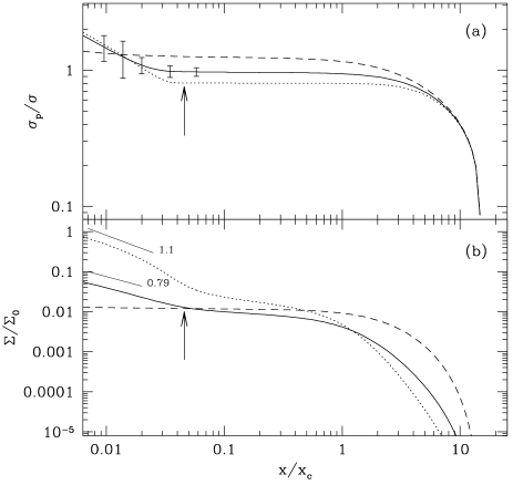
Figure 5: (a) Line-of-sight velocity dispersion profile and (b) projected surface density (normalized to the central value of the heavy remnants component) for the multimass model described in the text. Three components are shown: giant and turnoff stars (solid line), heavy dark remnants (dotted), lightest main sequence stars (dashed). The central logarithmic slope of $\Sigma$ are also reported for giants and heavy remnants. The vertical arrows indicate the BHIR radius. The error bars refer to simulated velocity dispersion measurements (see text).

Figure 6: Logarithmic slope of the space density of stars evaluated for the model stellar components (dots) inside the cusp region (at $x=0.01x_{\mathrm{c}}$) and fitted by the law $(m-0.29)^{0.33}+1$ (solid line). The short-dashed line is the $7/4$ value predicted in the single-mass context. The fit from the Baumgardt et al. (2004b) results (dotted line) and the Bahcall & Wolf (1977) relation (long-dashed) are also reported.

4 Black hole mass estimated from cluster profile

Exploiting equation  (19), we can now make a tentative estimate of the IMBH mass range in clusters, from their concentration and from the slope of the central surface brightness profile. To this purposes, the recent and detailed analysis made by NG06 of previous WFPC2/HST observations of 38 galactic globular clusters, provides the necessary set of data. Moreover, we also considered the controversial case of the cluster G1 in M31, for which $s$ is estimated by using the recent ACS/HST photometric profile published in Ma et al. (2007)(that gives the most recently updated value for $c$, as well) and the total mass and luminousity taken by Meylan et al. (2001).

From the whole list, 14 clusters were excluded (marked with ‘$\times$’ in the last column of Table 3) because they yield, from equation (19), a lower limit ($M_{\bullet,1}$) of the BH mass higher than the upper one ($M_{\bullet,2}$). All of core-collapsed clusters are in this subset, together with those having a steep central brightness profile ($s\ga 0.2$) in spite of being not very concentrated, like, e.g., NGC 6535 (that has $c=1.3$ and $s\simeq 0.5$). Of course, the presence of a IMBH cannot be completely ruled out for these clusters. It can only be stated that such a presence is incompatible with the stars phase-space distribution of the form given by equations (1) and (14). Moreover, there are 18 clusters (marked with ‘$\circ$’) having very low (or negative) central slope, for which $M_{\bullet,1}<100\,\mathrm{M}_{\odot}$; conservatively, they were considered as clusters without IMBH. This because the model is based on the assumption that $M_{\bullet}$ is much greater than any single stellar mass, so that one can assume, in good approximation, the IMBH to be at rest. Therefore, as regards these clusters, the model cannot provide sufficiently stringent and reliable predictions; accurate individual parametric fits would be necessary to this aim. Note, however, that the NG06 uncertainties on the measurements of $s$ are rather large. This error is not taken into account in the present analysis.

The relevant parameters of the remaining 7 candidate clusters are written in Table 4. Their predicted IMBH mass range is plotted both vs. the total cluster $V$-band luminosity and vs. the observed velocity dispersion (Fig. 7). It is apparent that $M_{\bullet}/M$ has only a weak dependence on $L$ while the BH mass tends to increase with $\sigma_{\mathrm{obs}}$. To quantify these trends, weighted least-squares fits were computed (following the prescriptions of Press et al., 1988, sect. 15.2) neglecting, for simplicity, the uncertainties both in $L$ and in $\sigma_{\mathrm{obs}}$. The resulting fits are

$$\log\left(\frac{M_{\bullet}}{M}\right)=(-1.2\pm 1.6)+(-0.33\pm 0.30)\log\left(\frac{L}{\mathrm{L}_{\odot}}\right)$$ (21)

with $\chi^{2}_{\mathrm{fit}}=0.63$ at a confidence level $P(\chi^{2}>\chi^{2}_{\mathrm{fit}})=0.99$, and

$$\log\left(\frac{M_{\bullet}}{\,\mathrm{M}_{\odot}}\right)=(1.7\pm 1.4)+(1.2\pm 1.2)\log\left(\frac{\sigma_{\mathrm{obs}}}{\textrm{km s}^{-1}}\right)$$ (22)

with $\chi^{2}_{\mathrm{fit}}=0.85$ and $P(\chi^{2}>\chi^{2}_{\mathrm{fit}})=0.97$. The cluster luminosity was chosen as an independent variable because its measure is much more reliable and directly linked to observations than the dynamically estimated total masses (Pryor & Meylan, 1993).

Assuming a uniform global mass-to-light ratio equal to that averaged among the candidate clusters, $\simeq 3.4(M/L)_{\odot}$, equation (21) gives $M_{\bullet}\sim 0.09(M/\,\mathrm{M}_{\odot})^{0.7\pm 0.3}\,\mathrm{M}_{\odot}$. This link is in agreement with the $M_{\bullet}\propto M$ relation between super-massive BHs in galactic nuclei and the bulge mass (Magorrian et al., 1998), and between the mass of compact nuclei and that of the host spheroid in nucleated early-type and dwarf galaxies (Côté et al., 2006; Wehner & Harris, 2006).

As regards relation (22), it is very different from the law $M_{\bullet}\sim\sigma_{\mathrm{obs}}^{4.8}$ found by Ferrarese & Merritt (2000) for galactic bulges (see also Gebhardt et al., 2000; Tremaine et al., 2002). The reason of this discrepancy can be understood by the same argument Ferrarese & Merritt presented to explain the relation they found: the $M_{\bullet}$ – $\sigma_{\mathrm{obs}}$ link is a consequence of the fundamental relation $M_{\bullet}\propto M$. In galaxies, this latter relation and the $M\sim L^{5/4}$ and $L\sim\sigma_{\mathrm{obs}}^{4}$ laws lead indeed to $M_{\bullet}\sim\sigma_{\mathrm{obs}}^{5}$. In globular clusters, on the other hand, the observed trends $M\sim L$ and $L\sim\sigma_{\mathrm{obs}}^{5/3}$ (Meylan & Heggie, 1997) yield, through equation (21), $M_{\bullet}\sim\sigma_{\mathrm{obs}}^{1.1}$, which is, in fact, compatible with the relation (22).

However, since in old globular clusters the secular collisional relaxation has certainly had a substantial influence on the dynamics within the core region, it is reasonable to expect only a weak correlation between $M_{\bullet}$ and the presently observed core velocity dispersion. Moreover, as discussed in sect. 3.1.1, it is rather improbable that $\sigma_{\mathrm{obs}}$ could provide a really reliable and accurate indication on the velocity dispersion in the inner cusp region; in fact, with the exception of G1, $N_{1}$ is rather low ($<60$) for the candidate clusters (see Table 4). Conversely, the cluster total mass, in spite of the tidal erosion, should keep a tighter link with the environmental conditions at the first stage of the cluster life (at least for massive clusters), when IMBHs formation are thought to have occurred (e.g. Gürkan et al., 2004).

To improve our capability of identifying the presence of IMBHs, it is important to search for other indicators that could be related to the gravitational influence of the compact object on the surrounding cluster stars. In this context, the presence of an extreme horizontal branch in the colour-magnitude diagram (CMD) may be a valid indicator, as we will see in the next Section.

Not surprisingly, however, another indication in favour of the presence of IMBHs at the centre of our candidate clusters, is that their $r_{\mathrm{c}}/r_{\mathrm{h}}$ ratio – as directly evaluated from the values listed in the Harris catalogue, see Table 4 – is significantly higher than the maximum value ($\sim 0.05$) suggested by Trenti (2006) for clusters that do not harbour IMBHs, and, consequently, do not experience the enhanced core expansion caused by their presence.

Note that three over five clusters that Baumgardt et al. (2005) indicate as possibly harbouring IMBHs, are in common with our candidates set (namely: NGC 6093, 6266, 6388). We consider the remaining two clusters, NGC 5286 and 5694, as non-candidate because they have $M_{\bullet,1}>M_{\bullet,2}$ (due to their relatively high concentration and slope); in this respect, notice that the core slope of the former cluster has been updated to an higher value in the final NG06 published list, compared with that reported by Baumgardt et al.. Furthermore, G1, NGC 2808 and 6205 are not considered by these authors, because they identify as candidate clusters just those with a non-collapsed core and with a central slope between $0.2$ and $0.3$, as suggested by the results of their simulations.

To conclude this section, it is worth noting the similarity of the surface brightness profiles reported by NG06 (plotted in their Fig. 7) with those illustrated here in Fig.s 1b and 5b. By inspecting those corresponding to our candidate clusters, the similarity is rather evident for M80 and M13. Indeed, these clusters show a clear transition between a core and a cusp region. Note that they are the only ones, in the NG06 set, in which this feature is clearly observed. Thus, more detailed individual studies, also through parametric fits of the profiles based on the model discussed here, certainly deserve to be carried out for them.

Figure 7: Upper panel: BH mass of the candidate clusters plotted vs. the observed central velocity dispersion (in km s^-1); lower panel: log of the ratio $M_{\bullet}/M$ plotted against total cluster luminosity. The dashed lines are the weighted least-squares fits $\log(M_{\bullet}/M)=-1.2-0.33\log(L/$L${}_{\odot})$ and $\log(M_{\bullet}/\,\mathrm{M}_{\odot})=1.7+1.2\log(\sigma_{\mathrm{obs}})$.

Table 3: Globular clusters in the NG06 set. $L$ is the total luminosity in the $V$-band evaluated from $M_{V}$ listed in the Harris catalogue. $c=$ cluster concentration (from the Harris catalogue; ‘:’ denotes a core-collapsed cluster). $s$ is the logarithmic slope (from NG06, with opposite sign). $M_{\bullet,1}/M$ and $M_{\bullet,2}/M$ are the lower and upper limits of $M_{\bullet}/M$ as from equation (19). $M$ is the total cluster mass taken, if available, from the parametric estimates in Pryor & Meylan (1993), while those marked with a ‘:’ are estimated by assuming a uniform global mass-to-light ratio $=2$. EHB₁ marked clusters are those with a Harris (1996) HB type $=0$. EHB₂ clusters are those having $\log({T_{\mathrm{eff}}}_{\mathrm{HB}})>4.3$ in the Recio-Blanco et al. (2006) list. Last column: $\bullet$ denotes a candidate cluster, ‘$\times$’ a cluster having $M_{\bullet,1}>M_{\bullet,2}$ and ‘$\circ$’ a cluster with $M_{\bullet,1}<100\,\mathrm{M}_{\odot}$. Not available data are indicated by ….

NGC number	$\log(L/\mathrm{L}_{\odot})_{V}$	$c$	$s$	$\log(M_{\bullet,1}/M)$	$\log(M_{\bullet,2}/M)$	$\log(M/\mathrm{M}_{\odot})$	EHB1	EHB2	case
104 (47 Tuc)	$5.7$	$2.03$	$0$	$-4.85$	$-3.01$	$6.1$			$\circ$
1851	$5.26$	$2.32$	$0.38$	$-0.442$	$-3.34$	$6.0$			$\times$
1904 (M79)	$5.12$	$1.72$	$0.03$	$-4.50$	$-2.65$	$5.2$	$\surd$	$\surd$	$\circ$
2298	$4.45$	$1.28$	$0$	$-4.85$	$-2.15$	$4.8$:		…	$\circ$
2808	$5.69$	$1.77$	$0.06$	$-4.15$	$-2.71$	$6.2$	$\surd$	$\surd$	$\bullet$
5272 (M3)	$5.5$	$1.84$	$0.05$	$-4.27$	$-2.79$	$5.8$		…	$\circ$
5286	$5.38$	$1.46$	$0.28$	$-1.60$	$-2.36$	$5.5$		…	$\times$
5694	$5.06$	$1.84$	$0.19$	$-2.65$	$-2.79$	$5.4$			$\times$
5824	$5.47$	$2.45$	$0.36$	$-0.67$	$-3.49$	$6.6$		$\surd$	$\times$
5897	$4.82$	$0.79$	$0.04$	$-4.39$	$-1.59$	$5.1$:		…	$\circ$
5904 (M5)	$5.46$	$1.83$	$-0.05$	$-5.43$	$-2.78$	$5.6$			$\circ$
6093 (M80)	$5.22$	$1.95$	$0.16$	$-2.99$	$-2.92$	$6.0$	$\surd$	$\surd$	$\bullet$
6205 (M13)	$5.41$	$1.51$	$0.1$	$-3.69$	$-2.41$	$5.8$	$\surd$	$\surd$	$\bullet$
6254 (M10)	$4.92$	$1.4$	$-0.05$	$-5.43$	$-2.29$	$5.4$	$\surd$	…	$\circ$
6266 (M62)	$5.61$	$1.7$	$0.13$	$-3.34$	$-2.63$	$5.8$		$\surd$	$\bullet$
6284	$5.12$	$2.5$:	$0.55$	$1.53$	$-3.54$	$5.4$			$\times$
6287	$4.88$	$1.6$	$0$	$-4.85$	$-2.52$	$5.2$:			$\circ$
6293	$5.04$	$2.5$:	$0.67$	$2.92$	$-3.54$	$5.6$		…	$\times$
6341 (M92)	$5.21$	$1.81$	$0.01$	$-4.73$	$-2.76$	$5.3$		…	$\circ$
6333 (M9)	$5.11$	$1.15$	$0$	$-4.85$	$-2.00$	$5.4$:		…	$\circ$
6352	$4.52$	$1.1$	$-0.02$	$-5.08$	$-1.95$	$4.8$:		…	$\circ$
6388	$5.7$	$1.7$	$0.13$	$-3.34$	$-2.63$	$6.2$			$\bullet$
6397	$4.58$	$2.5$:	$0.37$	$-0.56$	$-3.54$	$5.4$			$\times$
6441	$5.79$	$1.85$	$0.02$	$-4.62$	$-2.80$	$6.2$			$\circ$
6535	$3.83$	$1.3$	$0.5$	$0.95$	$-2.18$	$4.2$		…	$\times$
6528	$4.56$	$2.29$	$0.1$	$-3.69$	$-3.30$	$4.9$:		…	$\circ$
6541	$5.28$	$2$:	$0.41$	$-0.094$	$-2.97$	$5.6$		…	$\times$
6624	$4.93$	$2.5$:	$0.32$	$-1.14$	$-3.54$	$5.2$			$\times$
6626 (M28)	$5.20$	$1.67$	$-0.03$	$-5.20$	$-2.60$	$5.4$		…	$\circ$
6637 (M69)	$4.99$	$1.39$	$-0.09$	$-5.89$	$-2.28$	$5.3$:			$\circ$
6652	$4.60$	$1.8$	$0.57$	$1.76$	$-2.75$	$4.9$:			$\times$
6681	$4.78$	$2.5$:	$0.82$	$4.66$	$-3.54$	$5.2$		$\surd$	$\times$
6712	$4.93$	$0.9$	$-0.02$	$-5.08$	$-1.72$	$5.0$		…	$\circ$
6715 (M54)	$5.94$	$1.84$	$0.12$	$-3.46$	$-2.79$	$6.3$		…	$\bullet$
6752	$5.02$	$2.5$:	$0.03$	$-4.50$	$-3.54$	$5.2$	$\surd$	…	$\circ$
7078 (M15)	$5.6$	$2.5$:	$0.66$	$2.81$	$-3.54$	$6.3$	$\surd$	$\surd$	$\times$
7089 (M2)	$5.54$	$1.8$	$-0.05$	$-5.43$	$-2.75$	$6.0$		$\surd$	$\circ$
7099 (M30)	$4.90$	$2.5$:	$0.57$	$1.76$	$-3.54$	$5.3$			$\times$
G1	$6.31$	$2.01$	$0.06$	$-4.15$	$-2.99$	$7.0$	…	…	$\bullet$

Table 4: Candidate clusters set. $I_{0}$ is the central surface brightness estimated from $\mu_{V}$ in Harris (1996) using equation (5) in Djorgovski (1993). $r_{\mathrm{c}}$ is the core radius in pc, estimated from the angular value and the cluster distance listed in the Harris catalogue. $M_{\bullet,1}$ and $M_{\bullet,2}$ are in $\,\mathrm{M}_{\odot}$ and calculated using $M$ from Table 3. $\sigma_{\mathrm{obs}}$ is the central observed velocity dispersion taken from Pryor & Meylan (1993) or, marked with ‘:’, from Dubath, Meylan & Mayor (1997). $M/L$ is the mass-to-light ratio in solar unit. $r_{\mathrm{c}}/r_{\mathrm{h}}$ is the ratio between the core and the half-mass radius, directly estimated from Harris (1996). $N_{1}$ is the estimate of the no. of giants inside $x_{\mathrm{BH}}$ assuming $r_{\mathrm{BH}}=0.07r_{\mathrm{c}}$ in equation (20). The other symbols have the same meaning as in Table 3.

NGC number	$\log(L/\mathrm{L}_{\odot})$	$I_{0}$ (L⊙ pc-2)	$r_{\mathrm{c}}$	$M_{\bullet,1}$	$M_{\bullet,2}$	$M/L$	EHB1	EHB2	$\sigma_{\mathrm{obs}}($ km s${}^{-1})$	$r_{\mathrm{c}}/r_{\mathrm{h}}$	$N_{1}$
2808	$5.69$	$3\times 10^{4}$	$0.73$	$110$	$3.1\times 10^{3}$	$3.2$	$\surd$	$\surd$	$13.7\pm 1.4$	$0.34$	$31$
6093 (M80)	$5.22$	$2.94\times 10^{4}$	$0.44$	$10^{3}$	$1.2\times 10^{3}$	$6$	$\surd$	$\surd$	$13.4\pm 0.6$:	$0.23$	$11$
6205 (M13)	$5.41$	$6.68\times 10^{3}$	$1.7$	$130$	$2.4\times 10^{3}$	$2.4$	$\surd$	$\surd$	$6.62\pm 0.41$	$0.52$	$40$
6266 (M62)	$5.61$	$2.54\times 10^{4}$	$0.36$	$290$	$1.5\times 10^{3}$	$1.5$		$\surd$	$14.3\pm 0.4$:	$0.15$	$6$
6388	$5.7$	$5.31\times 10^{4}$	$0.35$	$720$	$3.7\times 10^{3}$	$3.2$			$18.9\pm 0.8$	$0.18$	$13$
6715 (M54)	$5.94$	$4.14\times 10^{4}$	$0.86$	$700$	$3.2\times 10^{3}$	$2.3$		…	$14.2\pm 1.0$	$0.22$	$59$
G1	$6.31$	$1.38\times 10^{5}$	$0.78$	$780$	$1.1\times 10^{4}$	$5.4$	…	…	$25.1\pm 1.7$	$0.12$	$160$

5 The IMBH – EHB connection

Let us assume that the loss of envelope mass is the dominant effect suffered by a giant during a close passage around the IMBH (‘tidal stripping’), and that it becomes an EHB star because of its uncovered underlying hotter layers (Rich et al., 1997; Alexander, 2005). Let $r_{\mathrm{tid}}=R_{*}(M_{\bullet}/m)^{1/3}$ be the distance from the IMBH below which the tidal interaction with a star (with radius $R_{*}$ and mass $m$) significantly perturbs its internal structure (see, e.g., Freitag & Benz, 2002; Baumgardt et al., 2006). The order of magnitude of the rate of tidal stripping events can be estimated as $S\simeq n_{0}\sigma_{0}\pi r_{\mathrm{tid}}^{2}(1+2GM_{\bullet}/r_{\mathrm{tid}}\sigma_{0}^{2})^{2}$, where $n_{0}$ and $\sigma_{0}$ are, respectively, the typical stellar number density and velocity dispersion in the cusp region, and where the gravitational focusing is taking into account in the estimate of the cross-section of the single stripping event (Freitag et al., 2006b).

For giants having $R_{*}\sim 100$ R_⊙ and $m=m_{1}$, one has $r_{\mathrm{tid}}\simeq 2.5\times 10^{-5}$ pc and taking, from the example discussed in section 3.1.1, $n_{0}\simeq 3N_{1}/4\pi r_{\mathrm{BH}}^{3}\simeq 2\times 10^{4}$ pc^-3, $\sigma_{0}\simeq 20$ km s^-1 and $M_{\bullet}=10^{3}\,\mathrm{M}_{\odot}$, one has $S\simeq 7\times 10^{-7}$ yr^-1, which means that of order of $100$ stripping events can occur within a HB stars lifetime ($\sim 10^{8}$ yr), generating a significant population of EHB stars. Incidentally, this population could have an integrated luminosity ($10^{2}$ – $10^{4}$ L_⊙, mainly in the $UV$ band) compatible with the far-UV excess showed by some – even metal-rich – clusters (e.g. NGC 6388, see Rich, Minniti & Liebert, 1993), while, on the contrary, it would be insufficient if one considered stripping events due to close encounters between stars only, as already pointed out by Rich et al. (1997). Thus, it is reasonable to expect that the existence of an EHB is favoured by the presence of an IMBH.

To test this hypothesis, we rely on the classification made in the Harris catalogue (revised on February 2003). This author re-analysed various set of CMD observations (mainly those by Piotto et al., 2002), in the intent of updating the Dickens (1972) HB type, introducing a new type ($=0$) to account for clusters having a prominent EHB. Thus, clusters with the HB type $=0$ are considered as having EHB (they are marked in the EHB₁ column of Table 3). Then, we study the probability distribution of finding a given number, $N_{\mathrm{EHB}}$, of clusters with an EHB, in a set as large as our candidate clusters set. However, for the sake of data homogeneity and because of the lack of direct observations of EHB stars, to the purpose of this analysis G1 is excluded from the candidates set.

A large number of subsets made up of 6 clusters each, were extracted at random from the NG06 list. Then, $N_{\mathrm{EHB}}$ was evaluated for each subset and a frequency distribution was computed (see the solid histogram in Fig. 8). The result is that the probability to get by chance a set of 6 clusters with $N_{\mathrm{EHB}}\geq 3$ (i.e. with $N_{\mathrm{EHB}}$ equal to or greater than that in our candidate clusters subset) is $\simeq 0.063$. This, from a statistical point of view, means that the hypothesis of the independence between the presence of an IMBH and the presence of an extended HB blue tail can be rejected at a confidence level $\ga 90$ percent.

However, the Harris new HB type was assigned to clusters with an high relative proportion of blue subdwarfs population in comparison with that at the redder side of the RR Lyrae region of the HB (Harris, private communication), whileas the determination of the presence of the EHB regardless of the other HB peculiarities would be more appropriate to our purposes. The various parameters defined by Fusi Pecci et al. (1993) to characterize the HB morphology are unsuitable as well, because their sample contains only very few clusters of the NG06 list. For these reasons, we chose considering the maximum effective temperature, ${T_{\mathrm{eff}}}_{\mathrm{HB}}$, evaluated by Recio-Blanco et al. (2006) for the HB stars of a clusters set that includes a significant part of the NG06 sample (see their table 1).

In this case, an EHB was considered as present when $\log({T_{\mathrm{eff}}}_{\mathrm{HB}})>4.3$ (i.e. ${T_{\mathrm{eff}}}_{\mathrm{HB}}\ga 20,000$ ^∘K, see e.g. Moehler 2001; Rosenberg, Recio-Blanco & García-Marín 2004). EHB clusters classified this way are signed in the ETB₂ column of Table 3. The visual inspection of the Piotto et al. (2002) CMDs – which the Recio-Blanco et al. (2006) evaluations are based on – confirms how in these clusters the EHB stars are clearly visible and reach downward a $V$ magnitude as faint as the turnoff point. While a fraction of the clusters with such an EHB have an Harris HB type $=0$, further clusters can be considered as owning EHBs. If one includes these clusters too, our candidates set has $N_{\mathrm{EHB}}=4$ and $P(N_{\mathrm{EHB}}\geq 4)\simeq 0.046$ (see Fig. 8, dashed histogram), consequently the confidence level rises to $\sim 95$ percent.

It is worth mentioning that the two candidate clusters (apart from G1) considered not to posses an EHB, show significant peculiarities in their HB. In particular, NGC 6388 shows an over-luminous blue HB (Rich et al., 1997; Raimondo et al., 2002; Catelan et al., 2006) and, similarly to what observed in M54 (Rosenberg et al., 2004), a blue HB extending anomalously beyond the theoretical zero-age HB (Busso, Piotto & Cassisi, 2004). As regards G1, we remind that there are some indirect indications suggesting the presence of a non-negligible population of EBH stars (Peterson et al., 2003) and that, at least, such a presence cannot be excluded according to the most recent CMD observations (Rich et al., 2005).

It can be also noticed that in the NG06 sample, there are 7 non-candidate clusters that possess EHB. This suggests that there might be other mechanisms – not related to the interaction with IMBHs – at work for the formation of EHB stars. However, 4 of those clusters are highly concentrated ($c>2.4$) or core-collapsed. This confirms that, whatever the formation mechanism is, it is favoured by an high density environment (Fusi Pecci et al., 1993; Buonanno et al., 1997). Nevertheless, the presence of such an environment at the present time is not a sufficient condition for the formation of an IMBH, which is closely linked to the initial central density instead. Gravothermal oscillations and collapse may have changed rapidly the former dynamical state, thus erasing the link with the initial environment. All this could explain the rather weak correlation found by Recio-Blanco et al. (2006) between ${T_{\mathrm{eff}}}_{\mathrm{HB}}$ and the collisional parameter they defined on the basis of the present dynamical conditions. Furthermore, the velocity dispersion used in the definition could be not representative of the higher actual value in the inner (not resolved) cusp region.

However, there are other alternative explanations for the presence of blue subdwarfs, which are not based upon tidal stripping (see Catelan, 2007, sections 7.3 – 7.4 and references therein). In this respect, notice that the helium self-enrichment – probably caused by multiple episodes of star formation – that in some clusters can explain the existence of EHB populations (e.g., in NGC 2808, see D’Antona et al., 2005; Piotto et al., 2007), could be also related to the presence of an IMBH. In fact, the IMBH could originate subsequent bursts of star formation, in a way similar – though on smaller scales – to what should occur into the accretion disk of super-massive BHs (e.g. Shlosman & Begelman, 1989; Collin & Zahn, 1999).

Figure 8: Probability distribution of finding $N_{\mathrm{EHB}}$ clusters having an extended blue tail, in a subset of 6 clusters randomly chosen from the NG06 set. The solid line histogram refers only to clusters with HB type $=0$, while in the dashed one those having $\log({T_{\mathrm{eff}}}_{\mathrm{HB}})>4.3$ are also taken into account. Our candidate clusters subset has $N_{\mathrm{EHB}}=3$ in the former case and $=4$ in the latter.

6 Conclusions

In this paper, the multimass isotropic and spherical King model has been extended to include the Bahcall & Wolf (1976) distribution function in the central region, so as to account for the presence of a central intermediate-mass black hole (IMBH). This self-consistent model generates surface brightness profiles that show a power-law behaviour around the centre and a core-like profile outwards. This latter is similar to a King profile with concentration $c<2$, though slightly steeper in the core region. The following features are particularly relevant:

$c$ decreases monotonically with the IMBH mass $M_{\bullet}$;

IMBHs with $10^{-3}M\la M_{\bullet}\la 10^{-2}M$, with $M$ the cluster mass, are compatible only with non-collapsed distributions ($c\la 2$);

the core surface brightness profiles exhibit a logarithmic slope $s\la 0.25$ for reasonably low IMBH masses ($M_{\bullet}\la 10^{-2}M$).

These features are in remarkable agreement with the results of recent collisional $N$-body simulations, which found that the IMBH causes a quick expansion of the a cluster core because of the enhanced collisional rate of exchange of kinetic energy both between stars of different masses (Baumgardt et al., 2005) and between single stars and hard binaries in 3-body encounters occurring in the black hole vicinity (Trenti et al., 2007). In particular, the slope of the profile of the core region in the simulated clusters attains values compatible with those found by our model. Moreover, the radius inside which the velocity dispersion profile is appreciably altered by the influence of the compact object ($\sim 3M_{\bullet}/M$ in units of the core radius) coincides with the value found by Baumgardt et al.. We can also confirm that a full cuspy density profile (similar to, e.g., that of collapsed clusters) can be associated only to a black hole with a unrealistically high mass, even higher than that of the host cluster itself.

A grid of models is then generated to derive possible trends of the IMBH mass with the morphological parameters. It is found that, in general, $12s-4.8\la\log(M_{\bullet}/M)\la-1.1c-0.69$. This mass range estimate is applied to a set of 38 galactic globular clusters recently re-analysed by Noyola & Gebhardt (2006) as well as to the case of G1 (in M31). It was found that seven clusters in this sample probably host an IMBH, namely: NGC 2808, NGC 6388, M80, M13, M62, M54 and G1. Among these, the M80 and M13 brightness profiles presented in Noyola & Gebhardt show the typical appearance of the cuspy-core behaviour reproduced by the model. It is worth noticing, moreover, that among the five clusters that Baumgardt et al. (2005) indicate as possibly harbouring IMBHs, M80, M62 and NGC 6388 are in common with our candidates set.

The scaling relations

$$M_{\bullet}\sim 0.09\left(\frac{M}{\,\mathrm{M}_{\odot}}\right)^{0.7}\,\mathrm{M}_{\odot},$$ (23)

$$M_{\bullet}\sim 50\left(\frac{\sigma_{\mathrm{obs}}}{\textrm{km s}^{-1}}\right)^{1.2}\,\mathrm{M}_{\odot},$$ (24)

are satisfied by our candidate clusters. Relation (23) is close to the $M_{\bullet}\sim M$ law found in larger scale systems (Magorrian et al., 1998; Côté et al., 2006; Wehner & Harris, 2006). None the less, relation (24) is significantly different for the analogous relation found in galaxies (Ferrarese & Merritt, 2000; Gebhardt et al., 2000; Tremaine et al., 2002), but the discrepancy can be understood by noting that the scaling law between the total mass and the central velocity dispersion for galaxies is very different from that followed by globular clusters.

Unfortunately, the uncertainties on the mass range estimates are in many cases rather large and, as a consequence, the presence of IMBHs on other clusters cannot be completely ruled out. They are mainly due to the uncertainties in the central observed projected velocity dispersion, and in the logarithmic slope measurements. For this reason, we plan to carry out individual studies on a representative cluster subset in the Noyola & Gebhardt (2006) sample, to infer the IMBH mass directly from the best parametric fit of their brightness profiles.

Nevertheless, this preliminary and ‘collective’ approach, permits to achieve an intriguing result: the presence of an extreme blue horizontal branch – determined according both to the Harris (1996) HB type index and to the maximum effective temperature of HB stars – is associated to the presence of the IMBH at a statistically significant level of confidence ($>90$ percent). Such a correlation is not surprising when one takes into account the high stellar density in the inner cusp region and the relatively high ratio between $M_{\bullet}$ and the single stellar mass, in calculating the rate of tidal stripping event in giants-IMBH close encounters.

This firmly suggests that the mass of the IMBH could be one of the ‘hidden’ parameters that are being searched for to explain the strong variability of HB morphology in clusters with the same metallicity and similar CMDs (the so-called ‘2nd parameter’ problem). For instance, the presence of a central IMBH in M13 and NGC 6388 could explain the origin of their extreme HB stars, while their absence in the respective ‘counterparts’ M3 and 47 Tuc is consistent with the the fact that, according to our analysis, IMBHs should not reside in these latter.

References

- Alexander (1999) Alexander T., 1999, ApJ, 527, 835
- Alexander (2005) Alexander T., 2005, Phys. Rep., 419, 65
- Amaro-Seoane et al. (2004) Amaro-Seoane P., Freitag M., Spurzem R., 2004, MNRAS, 352, 655
- Bahcall & Wolf (1976) Bahcall J.N., Wolf R.A, 1976, ApJ, 209, 214
- Bahcall & Wolf (1977) Bahcall J.N., Wolf R.A, 1977, ApJ, 216, 883
- Baumgardt et al. (2003a) Baumgardt H., Hut P., Makino J., McMillan S., Portegies Zwart S., 2003a, ApJ 582, L21
- Baumgardt et al. (2003b) Baumgardt H., Makino J., Hut P., McMillan S., Portegies Zwart S., 2003b, ApJ 589, L25
- Baumgardt et al. (2004a) Baumgardt H., Makino J., Ebisuzaki T., 2004a, ApJ, 613, 1133
- Baumgardt et al. (2004b) Baumgardt H., Makino J., Ebisuzaki T., 2004b, ApJ, 613, 1143
- Baumgardt et al. (2005) Baumgardt H., Makino J., Hut P., 2005, ApJ, 620, 238
- Baumgardt et al. (2006) Baumgardt H., Hopman C., Portegies Zwart S., Makino J., 2006, MNRAS, 372, 467
- Binney & Tremaine (1987) Binney J.J., Tremaine S., 1987, Galactic Dynamics. Princeton Univ. Press, Princeton, NJ
- Buonanno et al. (1997) Buonanno R., Corsi C. E., Bellazzini M., Ferraro F. R., Fusi Pecci F., 1997, AJ, 113, 706
- Busso et al. (2004) Busso G., Piotto G., Cassisi S., 2004, Mem. Soc. Astron. It., 75, 46
- Capuzzo Dolcetta et al. (2007) Capuzzo Dolcetta R., Leccese L., Merritt D., Vicari A., 2007, submitted to ApJ (astro-ph/0611205)
- Catelan (2007) Catelan M., 2007, in Valls Gabaud D., Chavez M., eds, Resolved Stellar Populations, ASP Conf. Series, in press. Astron. Soc. Pac., San Francisco (astro-ph/0507464)
- Catelan et al. (2006) Catelan M. et al., 2006, ApJ, 651, L133
- Cohn & Kulsrud (1978) Cohn H., Kulsrud R.M., 1978, ApJ, 226, 1087
- Collin & Zahn (1999) Collin S., Zahn J., 1999, A& A, 344, 433
- Colpi et al. (2005) Colpi M., Devecchi B., Mapelli M., Patruno A., Possenti A., 2005, in Interacting Binaries: Accretion, Evolution, and Outcomes. AIP Conf. Proc., Vol. 797. American Inst. of Phys., p. 205.
- Côté et al. (1995) Côté P., Welch D.L., Fischer P., Gebhardt K., 1995, ApJ, 454, 788
- Côté et al. (2006) Côté P. et al., 2006, ApJS, 165, 57
- D’Antona et al. (2005) D’Antona F., Bellazzini M., Caloi V., Fusi Pecci F., Galleti S., Rood R.T., 2005, ApJ, 631, 868
- Da Costa & Freeman (1976) Da Costa G. S., Freeman K. C., 1976, ApJ, 206, 128
- Dickens (1972) Dickens R.J. 1972, MNRAS, 157, 281
- Djorgovski (1993) Djorgovski S., 1993, in Meylan G., Djorgovski S., eds, Structure and Dynamics of Globular Clusters. ASP Conf. Ser. Vol. 50. Astron. Soc. Pac., San Francisco, p. 373
- Dubath et al. (1997) Dubath P., Meylan G., Mayor M., 1997, A& A, 324, 505
- Fabbiano (2006) Fabbiano G., 2006, ARA&A, 44, 323
- Ferrarese & Ford (2005) Ferrarese L., Ford H., 2005, Space Sci. Rev., 116, 523
- Ferrarese & Merritt (2000) Ferrarese L., Merritt D., 2000, ApJ, 539, L9
- Ferraro et al. (2003) Ferraro F. R., Possenti A., Sabbi E., D’Amico N., 2003, ApJ, 596, L211
- Frank & Rees (1976) Frank J., Rees M. J., 1976, MNRAS, 176, 633
- Freitag & Benz (2002) Freitag M., Benz W., 2002, A&A, 394, 345
- Freitag et al. (2006a) Freitag M., Amaro-Seoane P., Kalogera V., 2006a, ApJ, 649, 91
- Freitag et al. (2006b) Freitag M., Gürkan M.A., Rasio F.A., 2006b, MNRAS, 368, 141
- Fusi Pecci et al. (1993) Fusi Pecci F., Ferraro F.R., Bellazzini M., Djorgovski S, Piotto G., Buonanno R., 1993, AJ, 105, 1145
- Gebhardt et al. (2000) Gebhardt K. et al., 2000, ApJ, 539, L13
- Gebhardt et al. (2002) Gebhardt K., Rich R. M., Ho L. C., 2002, ApJ, 578, L41
- Gebhardt et al. (2005) Gebhardt K., Rich R.M., Ho L.C., 2005, ApJ, 634, 1093
- Gerssen (2004) Gerssen J., 2004, AN, 325, 84
- Gerssen et al. (2002) Gerssen J., van der Marel R.P., Gebhardt K., Guhathakurta P., Peterson R.C. Pryor C., 2002, AJ, 124, 3270
- Gerssen et al. (2003) Gerssen J., van der Marel R.P., Gebhardt K., Guhathakurta P., Peterson R.C. Pryor C., 2003, AJ, 125, 376
- Gunn & Griffin (1979) Gunn J.E., Griffin R.F., 1979, AJ, 84, 752
- Gürkan et al. (2004) Gürkan M.A., Freitag M., Rasio , 2004, ApJ, 604, 632
- Harris (1996) Harris W.E., 1996, AJ, 112, 1487
- Heggie & Hut (2003) Heggie D., Hut P., 2003, The Gravitational Million-Body Problem: A Multidisciplinary Approach to Star Cluster Dynamics. Cambridge University Press, Cambridge, NY.
- Hopman & Alexander (2006) Hopman C., Alexander T., 2006, ApJ, 645, L133
- Jones (1970) Jones B., 1970, AJ, 75, 563
- King (1966) King I.R., 1966, AJ, 71, 64
- Kormendy (2004) Kormendy, J., 2004, in Ho L. C., ed., Carnegie Observ. Astroph. Ser. Vol. 1, Coevolution of Black Holes and Galaxies. Cambridge Univ. Press, Cambridge, p. 1
- Lightman & Shapiro (1977) Lightman A.P., Shapiro S.L., 1977, ApJ, 211, 244
- Ma et al. (2007) Ma J. et al., 2007, MNRAS, 376, 1621
- Madau & Rees (2001) Madau P., Rees M.J., 2001, ApJ, 551, L27
- Magorrian et al. (1998) Magorrian J. et al., 1998, AJ, 115, 2285
- McLaughlin et al. (2006) McLaughlin D. E., et al. 2006, ApJS, 166, 249
- McNamara et al. (2003) McNamara B.J., Harrison T.E., Anderson J., 2003, ApJ, 595, 187
- Meylan & Heggie (1997) Meylan G., Heggie D.C., 1997, A&AR, 8, 1
- Meylan et al. (2001) Meylan G., Sarajedini A., Jablonka P., Djorgovski S.G., Bridges T., Rich R.M., 2001, AJ, 123, 830
- Merritt (2004) Merritt D., 2004, in Ho L. C., ed., Carnegie Observ. Astroph. Ser. Vol. 1, Coevolution of Black Holes and Galaxies. Cambridge Univ. Press, Cambridge, p. 263
- Milone et al. (2006) Milone A.P., Villanova S., Bedin L.R., Piotto G., Carraro G., Anderson J., King I.R., Zaggia S., 2006, A&A, 456, 517
- Miocchi (2006) Miocchi P., 2006, MNRAS, 366, 227
- Moehler (2001) Moehler S., 2001, PASP, 113, 1162
- Murphy et al. (1991) Murphy B.W., Cohn H.N., Durisen R.H., 1991, ApJ, 370, 60
- Noyola & Gebhardt (2006) Noyola E., Gebhardt K., 2006, AJ, 132, 447 (NG06)
- Noyola et al. (2006) Noyola E., Gebhardt K., Bergmann M., 2006, in Kannappan S. J. et al., eds, New Horizons in Astronomy: Frank N. Bash Symposium 2005. ASP Conf. Ser., Vol. 352. Astron. Soc. Pac., San Francisco, p.269
- Peebles (1972) Peebles P. J. E., 1972, ApJ, 178, 371
- Peterson et al. (2003) Peterson R.C., Carney B.W., Dorman B., Green E.M., Landsman W., Liebert J., O’Connell R.W., Rood R.T., 2003, ApJ, 588, 299
- Piotto et al. (2002) Piotto G. et al. 2002, A&A, 391, 945
- Piotto et al. (2007) Piotto G. et al. 2007, ApJ, 661, L53
- Portegies Zwart et al. (2004) Portegies Zwart S. F., Baumgardt H., Makino J., McMillan S.L., Hut P., 2004, Nat, 428, 724.
- Press et al. (1988) Press W.H., Teukolsky S.A., Vetterling W.T., Flannery B.P., 1988, Numerical Recipes in C: the Art of Scientific Computing. Cambridge Univ. Press, Cambridge, NY
- Preto et al. (2004) Preto M., Merritt D., Spurzem R., 2004, ApJ, 613, L109
- Pryor & Meylan (1993) Pryor C., Meylan G., 1993, in Meylan G., Djorgovski S., eds, Structure and Dynamics of Globular Clusters. ASP Conf. Ser., Vol. 50. Astron. Soc. Pac., San Francisco, p.357
- Raimondo et al. (2002) Raimondo G., Castellani V., Cassisi S., Brocato E., Piotto G., 2002, ApJ, 569, 975
- Rasio et al. (2006) Rasio F.A. et al., 2006, in van der Hucht K.A., ed., Highlights of Astronomy Vol. 14, Proc. XXVIth IAU General Assembly
- Recio-Blanco et al. (2006) Recio-Blanco A., Aparicio A., Piotto G., De Angeli F., Djorgovski S.G., 2006, A&A, 452, 875
- Rich et al. (1993) Rich R.M., Minniti D., Liebert J., 1993, ApJ, 406, 489
- Rich et al. (1997) Rich R.M. et al., 1997, ApJ, 484, L25
- Rich et al. (2005) Rich R.M., Corsi C.E., Cacciari C., Federici L., Fusi Pecci F., Djorgovski S.G., Freedman W.L., 2005, AJ, 129, 2670
- Richstone (2004) Richstone D., 2004, in Ho L. C., ed., Carnegie Observ. Astroph. Ser. Vol. 1, Coevolution of Black Holes and Galaxies. Cambridge Univ. Press, Cambridge, p. 280
- Rosenberg et al. (2004) Rosenberg A., Recio-Blanco A., García-Marín M., 2004, ApJ, 603, 135
- Schwarzschild (1979) Schwarzschild M., 1979, ApJ, 232, 236
- Shapiro (1985) Shapiro S.L., 1985, in Goodman J., Hut P., eds, Proc. IAU Symp. 113, Dynamics of Star Clusters. Reidel, Dordrecht, p. 373
- Shapiro & Lightman (1976) Shapiro S.L., Lightman A.P., 1976, Nat, 262, 743
- Shlosman & Begelman (1989) Shlosman I., Begelman M.C., 1989, ApJ, 341, 685
- Tremaine et al. (2002) Tremaine S., et al. 2002, ApJ, 574, 740
- Trenti (2006) Trenti M., 2006, submitted to MNRAS Letters (astro-ph/0612040)
- Trenti et al. (2007) Trenti M., Ardi E., Mineshige S., Hut P., 2007, MNRAS, 374, 857
- van den Bosch et al. (2006) van den Bosch R., de Zeeuw P.T., Gebhardt K., Noyola E., van de Ven G., 2006, ApJ, 641, 852
- van de Ven et al. (2006) van de Ven G., van den Bosch R. C. E., Verolme E. K., de Zeeuw P. T., 2006, A&A, 445, 513
- van der Marel (2004) van der Marel R.P., 2004, in L. C. Ho, ed., Carnegie Observ. Astroph. Ser. Vol. 1, Coevolution of Black Holes and Galaxies. Cambridge Univ. Press, Cambridge, p. 37
- Wehner & Harris (2006) Wehner E.H, Harris W.E., 2006, ApJ, 644, L17