The Stability of Double White Dwarf Binaries Undergoing Direct Impact Accretion

Abstract

We present numerical simulations of dynamically unstable mass transfer in a double white dwarf binary with initial mass ratio, $q=0.4$. The binary components are approximated as polytropes of index $n=3/2$ and the initially synchronously rotating, semi-detached equilibrium binary is evolved hydrodynamically with the gravitational potential being computed through the solution of Poisson’s equation. Upon initiating deep contact in our baseline simulation, the mass transfer rate grows by more than an order of magnitude over approximately ten orbits, as would be expected for dynamically unstable mass transfer. However, the mass transfer rate then reaches a peak value, the binary expands and the mass transfer event subsides. The binary must therefore have crossed the critical mass ratio for stability against dynamical mass transfer. Despite the initial loss of orbital angular momentum into the spin of the accreting star, we find that the accretor’s spin saturates and angular momentum is returned to the orbit more efficiently than has been previously suspected for binaries in the direct impact accretion mode. To explore this surprising result, we directly measure the critical mass ratio for stability by imposing artificial angular momentum loss at various rates to drive the binary to an equilibrium mass transfer rate. For one of these driven evolutions, we attain equilibrium mass transfer and deduce that effectively $q_{\rm crit}$ has evolved to approximately $2/3$. Despite the absence of a fully developed disk, tidal interactions appear effective in returning excess spin angular momentum to the orbit.

1 Introduction

Binaries containing compact components are of great current interest in astrophysics. For an up-to-date online review of the origin and evolution of binaries with all types of compact components see Postnov & Yungelson (2006). More specifically, for recent discussions of the orbital evolution and stability of mass transfer in the case of double white dwarf binaries, see Marsh et al. (2004) and Gokhale et al. (2007) (GPF). White dwarf stellar remnants represent the most frequent endpoint for stellar evolution and are therefore the most common constituents of binaries with compact components. When common envelope evolution occurs, a white dwarf pair can emerge as a sufficiently compact binary for gravitational radiation to drive the binary to a semi-detached state over an astrophysically interesting timescale. It has been estimated that $\sim 1.5\times 10^{8}$ double white dwarf (DWD) binaries exist within the Galaxy, of which approximately 1/3 are semi-detached (Nelemans, Yungelson & Portegies Zwart, 2001). The richness of these binaries will in fact impose a confusion-limited background for low-frequency gravitational wave detectors such as LISA (Hils, Bender & Webbink, 1990; Hils & Bender, 2000; Nelemans, Yungelson & Portegies Zwart, 2001). In this paper, we focus on the behavior of such double white dwarf binaries from the point where mass transfer ensues by evolving an equilibrium, semi-detached polytropic binary hydrodynamically. We leave the complex and interesting phenomena that bring such binaries into contact for other studies.

For a cool white dwarf star with mass well below the Chandrasekhar mass, gravity is balanced by the degeneracy pressure of non-relativistic electrons. For this study, we use a polytropic equation of state as an approximation to an idealized, cool white dwarf. For a polytrope with index $n=\frac{3}{2}$ and corresponding adiabatic exponent $\gamma=\frac{5}{3}$, the radius–mass relation is

$$R\propto M^{-1/3}.$$ (1)

If both components of a DWD binary have equal entropy (equal polytropic constants in the view of this approximate equation of state), it must be the less massive star that will reach contact with its Roche lobe first. Furthermore, Equation (1) indicates that the donor will expand upon mass loss to the accretor. This fact introduces the possibility that the resulting mass transfer may be dynamically unstable as the donor can expand well beyond its Roche lobe leading to catastrophic mass transfer.

If we neglect the angular momentum in the spin of the binary components and allow all the angular momentum contained in the mass transfer stream to be returned to the orbit by tides, we would expect that a binary composed of stars obeying the mass-radius relation in Equation (1) is stable provided that (Paczyński, 1967)

$$q=\frac{M_{D}}{M_{A}}\leq\frac{2}{3}=q_{\rm crit},$$ (2)

where $M_{D}$ and $M_{A}$ are, respectively, the masses of the donor and accretor. However, it is now well known that the exchange of angular momentum in DWD binaries dramatically alters their stability properties (Marsh et al. 2004; GPF). In many instances, the accretion stream will directly strike the surface of the accretor instead of orbiting to eventually form an accretion disk. As is well-known, a tidally truncated accretion disk can efficiently return the advected angular momentum to the orbit. However, in the direct impact accretion mode the stream spins up the accretor and it is not clear how much angular momentum can be returned to the orbit. We note that direct impact accretion is of relevance in cases where the binary components are of comparable size. In addition to DWD binaries, similar circumstances arise in the evolution of Algol binaries as well, for example.

The importance of the fundamental uncertainty in the efficiency of tidal coupling was highlighted in the population synthesis calculations of Nelemans, et al. (2001). In the idealized case where no angular momentum is lost in the accretor’s spin (as would hold for the prediction in Equation 2), approximately $20\%$ of DWD binaries can survive mass transfer to become long-lived, AM CVn-type binaries. On the other hand, if none of the accretor’s spin angular momentum is returned to the orbit, the effective mass ratio for stable mass transfer is reduced significantly from the expectation reflected in Equation (2) and very few AM CVn can arise from a DWD progenitor. Rather, most DWD binaries would be disrupted shortly after becoming semi-detached, followed by a disk or common envelope phase and ending in merger. In the event that the total system mass exceeds the Chandrasekhar limit, the catastrophic merger would result in a, perhaps anomalous, type Ia supernova.

We present here a series of evolutions of an initially semi-detached DWD binary model with an initial mass ratio of $q=0.4$. The accretor is sufficiently large for the resulting mass transfer stream to strike the accretor directly. This binary thus begins its evolution as a stable system with respect to mass transfer in the limiting case of efficient tidal coupling but will be unstable if direct impact accretion removes angular momentum from the binary orbit. In §2, we present our baseline evolution of this model through 43 orbits and demonstrate that while mass transfer does grow rapidly in the initial phase, the binary separates and the mass transfer rate then declines allowing the binary to survive. To further investigate this result, we measure the mass ratio for stability to dynamical mass transfer in §3 by repeating our initial simulation with various artificial driving rates of angular momentum loss. We find that, effectively, this model binary transitions from unstable mass-transfer to stable mass transfer; at late times it appears to behave like a system that returns angular momentum rapidly to the binary orbit despite the absence of a tidally truncated accretion disk. In §4, we present a simple analysis for understanding these evolutions in terms of orbit-averaged equations. This analysis demonstrates that, in our simulations, the rate of change in the spin of the accretor saturates and subsequently the mass transfer rate begins to subside. In the concluding §5, we summarize our results and highlight some important points that may limit the application of our results to real DWD binaries.

2 Baseline Evolution of the Q0.4 Binary

We begin by considering the numerical evolution of a polytropic binary with an initial mass ratio of $q=0.4$. The computational tools for performing this simulation and for generating the initial data have been described previously in Motl, Tohline & Frank (2002) (MTF) and include the important modifications described in D’Souza et al. (2006) (DMTF) that enable long-term evolutions of binary models. In the evolution, we solve the equations for ideal, Newtonian hydrodynamics while simultaneously solving Poisson’s equation to give a consistent gravitational potential at every timestep in the evolution.

The initial data describe an $n=\frac{3}{2}$ polytropic binary that is synchronously rotating on a circular orbit. The relevant parameters for the $q=0.4$ (hereafter Q0.4) model are listed in Table 1. As in DMTF, we use polytropic units where the radial extent of the computational grid for the SCF model, the maximum density of one binary component and the gravitational constant are all unity. In Table 1, we list initial values for the mass ratio $q_{0}$, separation $a_{0}$, angular frequency $\Omega_{0}$, total angular momentum $J^{\rm tot}_{0}$ and the offset $R_{\rm com}$ between the system center of mass and the origin of the evolution grid (which is much less than the grid spacing used $\Delta R=\frac{1}{127}\approx 7.87\times 10^{-3}$). We also have tabulated values for the component’s mass $M_{i}$, maximum density $\rho^{\rm max}_{i}$, polytropic constant $\kappa_{i}$, stellar volume $V_{i}$ and Roche lobe volume $V^{RL}_{i}$.

Note in particular that the polytropic constants, $\kappa_{i}$, are not equal for the two components and that the volume of the more massive star, ultimately the accretor, exceeds the volume of the donor which is nearly in contact with its Roche lobe. In the formulation of the SCF code we have used to create this initial data (see MTF for details), we must specify parameters that do not directly correspond to a desired binary with a prescribed mass or entropy ratio. The Q0.4 model was generated by trial and error and while it posses an interesting mass ratio, its components do not conform to the desired mass-radius relation of Equation (1) relative to one another due to the difference in polytropic constants. We have begun to develop an improved SCF technique that is capable of enforcing a desired mass ratio and mass-radius relation a priori but for now we proceed with the Q0.4 model as it stands. Though the accretor is well inside its Roche lobe initially, and becomes even more confined in its potential well as the evolution proceeds, the reader is encouraged to be mindful of the caveat that the accretor’s size may accentuate gravitational torques on the binary leading the system to be more stable to dynamical mass transfer than real DWD binaries of the same initial mass ratio.

To make this cautionary note concrete, from Table 1 one can conclude that the effective radius of the accretor is approximately 1.6 times larger than it should be based upon the mass radius relation in Eq. (1) due to the differing polytropic constants of the two components. The magnitude of the tidal field of the accretor should scale as $\left(R_{A}/a\right)^{6}$ (see for example Campbell (1984) or Zahn (2005)). The accretor’s tidal field in this specific binary model is thus overestimated by a factor of approximately 17.

Table 1: Initial Parameters for Model Q0.4

System	Initial SCF	Component
Parameter	Value	Parameter	Donor	Accretor
$q_{0}$	0.4085	$M_{i}$	$6.957\times 10^{-3}$	$1.703\times 10^{-2}$
$a_{0}$	0.8169	$\rho^{\rm max}_{i}$	0.71	1.0
$\Omega_{0}$	0.2112	$\kappa_{i}$	$1.904\times 10^{-2}$	$3.119\times 10^{-2}$
$J^{\rm tot}_{0}$	$7.794\times 10^{-4}$	$V_{i}$	$6.180\times 10^{-2}$	0.1041
$R_{\rm com}$	$2.669\times 10^{-6}$	$V^{RL}_{i}$	$6.204\times 10^{-2}$	0.2154

The initial binary model described above is introduced into the hydrodynamics code and evolved on a cylindrical mesh with 162 radial by 98 vertical by 256 azimuthal zones. The evolution is performed in a rotating frame of reference where the frame frequency is taken to be the angular frequency consistent with the initial data, $\Omega_{0}$ and this frame frequency is kept fixed during the evolution. The center of mass correction described in DMTF is used and we drain angular momentum from the binary to drive the donor into deep contact with its Roche lobe. Specifically, we remove angular momentum as described in DMTF at a rate of $1\%$ per orbit for the first 1.6 orbits where the orbital time, $P_{0}=2\pi/\Omega_{0}$. The initial driving tightens the binary, causing a well-resolved accretion stream to form. This speeds up the numerical evolution and in the event of dynamically unstable mass transfer, the mass transfer rate will rapidly grow to a large amplitude in any event.

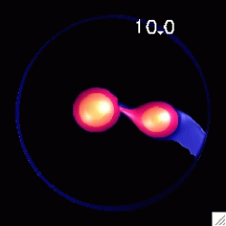
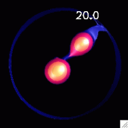
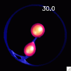
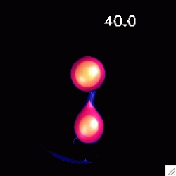
Figure 1: Four still frames from the baseline evolution of the Q0.4 binary, viewed from above along the rotational axis. The images show, starting in the upper left hand corner, the binary at 10, 20, 30 and 40 times the initial binary period. The innermost shell depicts a surface of constant density at $0.5\;\rho_{\rm max}$ while the yellow, red and blue surfaces correspond to density levels of $0.1,10^{-3}$ and $10^{-5}\;\rho_{\rm max}$. In the online version, we present an MPEG movie of the entire evolution through 43 orbits.

Images from the baseline Q0.4 evolution are shown in Figure 1 at 10, 20, 30 and 40 $P_{0}$. The binary is viewed from above with counter-clockwise motion corresponding to the binary advancing in the, initially, co-rotating frame. The different colored shells are isopycnic surfaces corresponding to density levels of $0.5,0.1,10^{-3}$ and $10^{-5}$ of the maximum density from the innermost to outermost, blue, surface. At 10 $P_{0}$, the mass transfer rate is near its peak value, corresponding to approximately $0.4\%$ of the donor’s initial mass per orbit. In the subsequent frames, the binary separates (moves clockwise about the rotational axis), the mass transfer stream diminishes and the binary attains stable, long-lived mass transfer with a rather gentle evolution.

Two numerical artifacts are apparent in these images and warrant further discussion. In addition to the mass transfer stream at L1, there is an outflow of low density material from the backside of the donor. This outflow is a numerical error and its presence establishes a floor level for the mass transfer rate that is resolved and corresponds to physical mass loss from the donor (see DMTF for further discussion). In our baseline simulation, the mass flux at L1 dominates this numerical effect by over an order of magnitude. Integrated over the entire evolution, less that 0.1% of the initial system mass exits the computational domain through this outflow. In addition, we enforce a vacuum level on the mass density of $10^{-10}$ for numerical stability. The vacuum level should be compared to the maximum density of order 1 and the characteristic density at the edge of the stars which is approximately $10^{-5}$. Enforcing this vacuum level adds mass to the grid at a rate nearly equal to the outflow with the net effect that the total mass increases by $4\times 10^{-6}$ relative to its initial value over the baseline evolution. We also wish to discuss the ring of material that forms when the donor’s outflow interacts with the grid boundary. We implement simple outflow boundary conditions (MTF) that are mathematically consistent only in the case where the fluid velocity normal to the boundary is supersonic (please see Stone and Norman 1992 for further discussion of boundary conditions for Eulerian codes). Using our simple formulation of the boundary conditions as opposed to a characteristic treatment allows material to accumulate against the grid edge but its presence does not appear to influence our results.

We examine the baseline evolution in more detail with the plots shown in Figure 2. The mass ratio decreases throughout the simulation, falling by $\sim 12\%$ through the 43 orbits of the evolution. The smoothed mass transfer rate is shown in the top right panel of Figure 2. The donor loses mass at a rapidly accelerating rate over the first 10 orbits of the evolution, the mass-transfer rate then peaks and begins to diminish to a nearly constant level from about 25 orbits through the end of the evolution. Modulations in the orbit, reflected in a rather complicated pattern in the ellipticity of the nearly circular orbit, result in a varying depth of contact and hence a varying mass transfer rate in the last quarter of the evolution. The orbital separation is shown in the middle left panel of Figure 2. The initial driving causes the binary to contract but soon the binary begins to expand and the expansion continues throughout the run. The baseline simulation is stopped after 43 orbits because the binary has separated to the point that the components approach the boundary of the computational domain.

Figure 2: Relevant binary parameters through the baseline evolution of the Q0.4 system; time is shown in units of $P_{0}$. Beginning in the upper left hand panel, we show the binary mass ratio $q=M_{D}/M_{A}$. The mass transfer rate, normalized to $\dot{M}_{\rm ref}=M_{D}/P_{0}$ is shown in the upper right hand panel. The mass transfer rate has been averaged with box-car smoothing over 3 orbital period intervals. In the middle row we show the orbital separation, normalized to its initial value, and the orbital angular momentum, normalized to the system’s initial, total angular momentum $J_{0}^{\rm tot}$. In the bottom row we show the spin angular momentum of the accretor (left panel) and donor (right panel) where each has been normalized by $J_{0}^{\rm tot}$.

To complete the description of the baseline evolution, we also plot several angular momentum components of the binary system in Figure 2. The orbital angular momentum is shown in the middle right panel and we see that the orbital angular momentum is removed by the initial driving and falls further due to mass transfer and direct impact accretion. Correspondingly, the accretor is spun up, as shown in the bottom left panel of Figure 2. The donor does not significantly change its spin angular momentum during the evolution as shown in the bottom right panel of Figure 2. Interestingly, the accretor’s spin appears to saturate at about 20 orbits, despite the fact that mass transfer continues. We will return to this point in §4.

To summarize, mass transfer grows rapidly by approximately an order of magnitude in the initial ten orbits of the evolution. During this initial phase, the simulation largely follows the expectations for direct impact accretion: the binary loses angular momentum from the orbit which spins up the accreting star and the orbital separation begins to expand once the mass transfer has grown sufficiently (see Equation (6) and discussion in GPF). Initially, $q>q_{\rm crit}\sim 0.2$ because of the effects of direct impact (Marsh et al. (2004); GPF), so the mass transfer is unstable and very little, if any, of the angular momentum of the stream is returned to the orbit. However, at approximately ten orbits, the mass transfer rate begins to decline and eventually the accretor’s spin stabilizes while the binary continues to expand. At the time that the mass transfer rate begins to decline, the binary mass ratio has fallen to $q=0.396$ (from it’s initial value of 0.409 as listed in Table 1). This demonstrates that, for this model, the mass transfer has stabilized. This in turn implies that the critical mass ratio for stability against dynamical mass transfer must have grown to a value $q_{\rm crit}\geq 0.396$, which is the value of $q$ at 10 orbits. Although there is no driving at this stage of the evolution, it is possible, due to the flow induced in the donor star towards the $L1$ point, that mass transfer may continue even after $q<q_{\rm crit}$. The above considerations suggest that $q_{\rm crit}$ evolves and increases once the accretor spin saturates and a significant part of the angular momentum carried by the stream is returned to the orbit. We can not, based on this simulation, exclude the possibility that stability returns to the binary at an even earlier point in its evolution. Due to finite numerical resolution we can only treat semi-detached systems with a mass transfer rate above a certain floor value and thus the entire evolution of a real DWD binary undergoing unstable mass transfer at rates below our resolution limit is inaccessible. It is in this sense that our simulation demonstrates a bound on the fate of the system; the return to stability with the provision that the mass transfer grows to amplitudes such as those shown in Figure 2. In the next section, we perform additional numerical experiments to directly measure the value of $q_{\rm crit}$ to improve upon the lower bound we have inferred from the fact that the mass transfer rate declines. The lower bound is still of interest though, as it is significantly higher than the value expected for negligible tidal coupling during direct impact accretion of $q_{\rm crit}\sim 0.2$ (Marsh et al. (2004); GPF).

3 Driven Evolutions of the Q0.4 Binary

We now attempt to directly measure the effective value of the critical mass ratio for stability against dynamical mass transfer, $q_{\rm crit}$, by imposing an artificial driving loss of angular momentum. If the model binary attains its equilibrium mass transfer rate, that rate should be simply related to measurable quantities from the simulation and the unknown value $q_{\rm crit}$ through (see GPF)

$$\dot{M}_{\rm eq}=M_{D}\frac{\left(\dot{J}/J^{\rm tot}\right)_{\rm driving}}{\left(q_{\rm crit}-q\right)}.$$ (3)

At a time of 7.7 orbits into the evolution, we impose one of three constant driving rates as listed in Table 2. This time was chosen because it corresponds to the deepest degree of contact attained during the baseline simulation before the rate of increase of the mass transfer begins to slow down. The baseline evolution from the previous section, where no additional driving is imposed, is included in this section as simulation Q0.4A. The additional driving is imposed in the remaining three simulations while the mass transfer rate is still growing in the baseline calculation. Consider the Q0.4B evolution with a driving rate of $1.0\times 10^{-3}$. If $q_{\rm crit}$ followed from the limit of effective tidal coupling, we would expect an equilibrium mass transfer rate at ten orbits of approximately $0.4\%$ of the donor’s initial mass per orbit. However, if $q_{\rm crit}=0.4$, for example, we would instead find a very high equilibrium mass transfer rate at ten orbits of $\sim 10\%$ of the donor’s initial mass per orbit. Recall that from our results in the previous section, we know that $q_{\rm crit}$ becomes $\geq 0.396$. The driving rates of angular momentum loss listed in Table 2 are constant (independent of the binary or stellar parameters) and far exceed the plausible magnitude for gravitational radiation or magnetic braking in real binary systems. As we have a limited range of reliable mass transfer rates that can be simulated, so too does this imply a range of effective driving rates available to manipulate the evolution of the binary. The expression for the equilibrium mass transfer rate in terms of the effective value of $q_{crit}$ in Eq. (3) does not require the time scales for mass transfer or driving correspond with known physical mechanisms such as the emission of gravitational radiation. It is merely sufficient for the mass transfer to have reached its equilibrium value given the applied driving loss of angular momentum.

Table 2: Driving rates for $t>7.7P_{0}$

Simulation	$\left(\dot{J}/J^{\rm tot}\right)_{\rm driving}$
A (Baseline)	0.0
B	$-1.0\times 10^{-3}$
C	$-2.0\times 10^{-3}$
D	$-5.0\times 10^{-3}$

Visualizations of the three driven evolutions are shown in Figure 3. The images depict the density distribution at each quarter of the respective evolution and show that as the artificial driving rate is increased, the mass transfer becomes progressively more extreme. The Q0.4B and Q0.4C evolutions follow the general pattern of the Q0.4A evolution in that the mass transfer rate grows rapidly yet the binary survives to expand to larger separations and the mass transfer event subsides. However, in the Q0.4C run, the accretor becomes highly distorted due to the accreted mass. In the final simulation, at the highest driving rate of $5\times 10^{-3}$, the mass transfer grows to a very high level and the donor is torn apart by tidal forces before it can escape to larger separations.

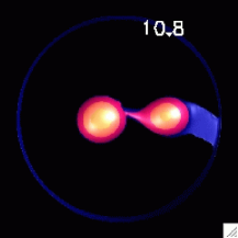
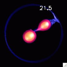
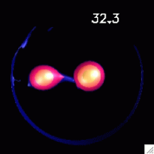
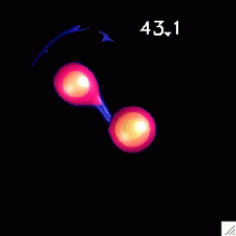
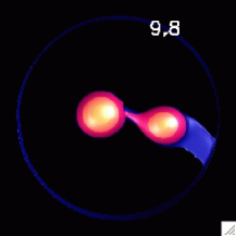
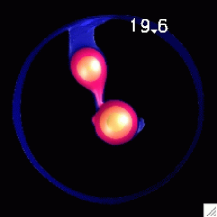
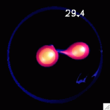
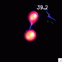
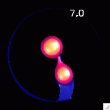
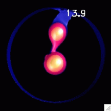
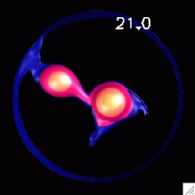
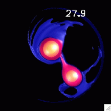
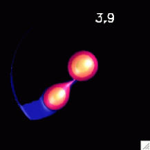
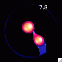
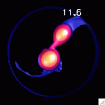
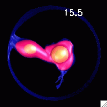
Figure 3: The four rows, from top to bottom, show snapshots taken during the four evolutions Q0.4A, Q0.4B, Q0.4C, and Q0.4D. The snapshots show the same isopycnic surfaces as in Fig. 1, viewed from above the orbital plane, at approximately, from left to right, $T_{\rm f}/4$, $T_{\rm f}/2$, $3T_{\rm f}/4$, and $T_{\rm f}$, where $T_{\rm f}$ identifies the time at which each evolution was terminated. Each frame is labeled with the corresponding time in units of $P_{0}$. In the online edition, we present MPEG movies showing the complete evolutions.

As shown in Figure 4, the trajectories of the key binary parameters confirm the impression that is drawn from a visual inspection of the images of the individual runs. (The key parameters displayed in the six panels of Figure 4 are the same as in Figure 2 and the trajectories for the baseline evolution Q0.4A, shown in Figure 2, have been re-drawn as black curves for comparison.) The behavior of model Q0.4D, that was driven at the largest rate, is plotted as the red curves in the six panels of Figure 4. The binary mass ratio plunges catastrophically as the advected angular momentum carried by the accretion stream spins up the accretor. In this simulation, the binary separation falls and then tries to expand but, by this point, the donor star has insufficient mass to bind the star and the donor is shredded by tidal forces. At the two lower driving rates we have considered, the binary is able to remain intact. The green curves correspond to the Q0.4C binary which was driven at $0.2\%$ from 7.7 orbits onwards. The high mass transfer rate causes the binary to rapidly separate and even in this case, the accretor’s spin angular momentum stalls. While this evolution is of note because the binary survives, the system does not attain steady state mass transfer and rapidly encroaches on the grid boundary, forcing us to end the evolution.

Results from the binary driven at the lowest rate, the Q0.4B binary which was driven at $0.1\%$ from 7.7 orbits onwards, are shown as the blue curves in Figure 4. This evolution closely follows the results we have presented in §2 for the baseline evolution: The mass transfer rate rises initially, then falls to an approximately steady level as the binary expands. At the same time, the binary loses orbital angular momentum into the spin of the accreting star which again appears to saturate and become approximately constant.

If we take the mass transfer rate in the Q0.4B binary from approximately 30 orbits onwards as the equilibrium mass transfer rate, $\dot{M}_{\rm eq}$, we see immediately that the low mass transfer rate in this phase is not consistent with a small value for $q_{\rm crit}\sim 0.4$. Taking the driving rate at $10^{-3}$ and using values for the mass ratio and mass transfer rate from the plots in Figure 4 in Equation (3), we deduce that $q_{\rm crit}\sim 0.7$. This value is consistent with the expectation from Equation (2) for very efficient return of angular momentum as would be the case when an accretion disk is present that fills most of the accretor’s Roche lobe. No such disk develops in evolution Q0.4B, however.

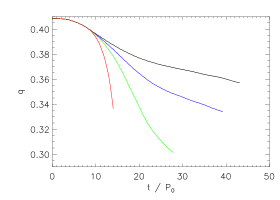
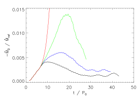
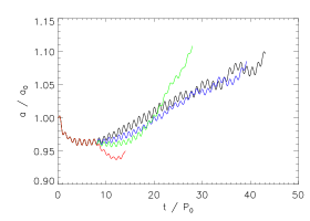
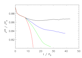
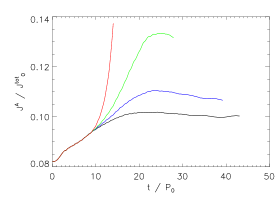
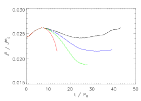
Figure 4: Binary parameters, as plotted in Figure 2, for the baseline evolution Q0.4A (black curves) and the three driven evolutions Q0.4B (blue curves), Q0.4C (green curves) and at the highest driving rate considered for the Q0.4D evolution (red curves).

For this model binary, with an initial mass ratio intermediate between the plausible maximum and minimum values of $q_{\rm crit}$, we find that it behaves, in the steady phase of the evolution, in a manner more consistent with that case of maximum efficiency for tidal coupling. The advected angular momentum that spins up the accretor is returned to the binary orbit on a timescale comparable to the mass transfer timescale itself. We therefore conclude that in many instances, DWD binaries could survive to reach a long-lived AM CVn state if hydrodynamics and gravity were the only processes in play. To understand this curious result in more detail, we turn in the next section to analyze the simulation output from the point of view of a relatively simple, orbit-averaged equation of motion for the binary.

4 Comparison to Expectations from the Orbit-Averaged Equations

In the previous sections, we have demonstrated the surprising resiliency of a polytropic binary that undergoes direct impact accretion. We have found that, in terms of dynamics, the binary behaves as if there were a mechanism in the system that can effectively return angular momentum from the accretor’s spin to the binary orbit. We have also observed in the three simulations of this binary where the donor star survives, that the accretor does not spin up indefinitely. To the contrary, the spin angular momentum of the accretor appears to saturate despite the fact that mass transfer continues to bring high-angular momentum material onto the accretor.

To understand this behavior, we turn to a simplified orbit-averaged equation to analyze the different physical effects that are competing to determine the fate of the binary. For general background on orbit-averaged equations and their application to the orbital evolution of DWD see GPF. We first decompose the angular momentum of the binary into the orbital angular momentum of each star’s center of mass and the spin angular momentum of each star about their respective center of mass as follows

$$J^{\rm tot}=J_{\rm orb}+J_{A}+J_{D}.$$ (4)

For a point mass binary, we may use Kepler’s third law to express the orbital angular momentum as

$$J_{\rm orb}=M_{A}M_{D}\sqrt{\frac{G\;a}{M_{A}+M_{D}}},$$ (5)

where $a$ is the orbital separation and $G$ is the universal gravitational constant. Combining Equations (4) and (5) and then logarithmically differentiating with respect to time we obtain

$$\frac{\dot{a}}{2a}=\left(\frac{\dot{J}_{\rm orb}}{J_{\rm orb}}\right)_{\rm driving}-\left(\frac{\dot{J}_{A}}{J_{\rm orb}}+\frac{\dot{J}_{D}}{J_{\rm orb}}\right)-\frac{\dot{M}_{D}}{M_{D}}\left(1-q\right),$$ (6)

where we have assumed conservative mass transfer.

The left hand side in Equation (6) reflects the trajectory of the mean orbit and this is equated to several competing terms on the right hand side. Since $\dot{J}_{\rm orb}$ is negative, the driving term tends to shrink the binary while the exchange of mass tries to expand the system since the mass ratio is less than unity. Recall that $\dot{M}_{D}$ is by its nature a negative quantity. On the other hand, an increase in the spin angular momentum of either the donor or accretor drives $\dot{a}$ to negative values as the angular momentum had to ultimately come at the expense of the binary orbit.

We apply Equation (6) by simply substituting the simulation data (as appears in the plots of Figure 4) for all the terms. Time derivatives are evaluated through numerical differentiation and the natural scale of the terms is the initial binary frequency, $\nu_{0}=1/P_{0}$. For example, the term on the left hand side is proportional to the rate at which the binary separation changes as a percentage rate per orbital period, $P_{0}$. The data values and their time derivatives have been smoothed with a sliding boxcar average with a width of three $P_{0}$, as was used previously to construct the mass transfer rates in Figures 2 and 4.

The terms appearing in Equation (6) are plotted as a function of time for the four simulations in Figure 5; each row in the figure represents a separate simulation where Q0.4A is across the top and Q0.4D is across the bottom. The black curves in both the left-hand panels and the right-hand panels of Figure 5 display the behavior of the left-hand side of Equation (6), while the total sum of the terms on the right-hand side of that equation is shown in red on the right-hand panels of the figure. The two sides of the equation do indeed track each other, with the orbit oscillating (due to epicyclic motion) about the mean dictated by the right hand side. The behaviors of the individual terms that contribute to the right-hand side of Equation (6) are displayed in the middle column of Figure 5. The driving loss of angular momentum appears in orange and is given by a superposition of step functions. The initial driving to force the binary into contact appears in all four simulations at a $1\%$ rate of loss for the initial 1.6 orbits. At 7.7 orbits, the additional driving terms are switched on at the rates given in Table 2 for simulations Q0.4B - Q0.4D.

The mass transfer term, that is, the last term appearing on the right hand side of Equation (6), is plotted (including the sign) as the green curves in Figure 5. This term is indeed stabilizing and tries to force the binary separation to expand. The spin terms are shown in blue with the donor’s spin (again, including the sign) plotted as dashed blue lines near zero amplitude and the accretor’s spin contribution plotted as solid blue curves.

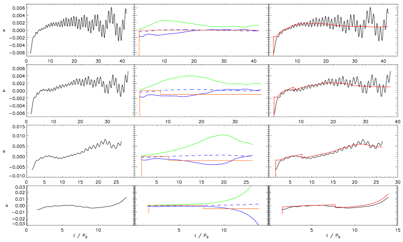
Figure 5: Terms appearing in the orbit averaged Equation 6 for the four evolutions presented in this paper. The four rows, from top to bottom, correspond to evolutions Q0.4A, Q0.4B, Q0.4C, and Q0.4D. The left-hand side of Equation 6, which traces variation in orbital separation, is shown as the oscillatory black curve on the left column. The central column shows the individual terms on the right-hand side of the same equation: the driving angular momentum term is shown in orange and the mass transfer term is plotted in green; the accretor and donor spin terms are plotted as a solid and a dashed blue line respectively. The right column shows superimposed the left-hand side of the equation (black) and the sum of all terms on the right hand side (red), to demonstrate that Equation 6 is indeed satisfied on average. The terms in Equation 6 have a dimension of inverse time and here, time is measured in units of the initial orbital period. The ordinate $\nu$ is plotted in units of $P_{0}^{-1}$.

Table 3: Reference times

Simulation	$\left(\frac{\dot{J}}{J}\right)_{\rm driving}$	Time of Minimum $\left(-\frac{\dot{J}_{A}}{J_{\rm orb}}\right)$	Time of Maximum $\left(-\frac{\dot{M}_{D}}{M_{D}}\left(1-q\right)\right)$
Q0.4A	0.0	7.94 $P_{0}$	10.12 $P_{0}$
Q0.4B	$1\times 10^{-3}$	14.29 $P_{0}$	17.34 $P_{0}$
Q0.4C	$2\times 10^{-3}$	17.37 $P_{0}$	19.56 $P_{0}$

The simulated binaries satisfy Equation (6) to a surprising accuracy. The black curves closely track the effective driving within the binary - the sum of all terms on the right hand side plotted in red - even for the extreme mass transfer of the Q0.4D simulation. For this run, the mass transfer and accretor spin terms each diverge in opposite directions and yet the binary separation tracks their combined effect closely. In the remaining three simulations, the binary separation oscillates about the effective driving as eccentricity builds up in the orbit.

We also observe that while the spin-up of the accretor tries to destabilize the binary, this term makes its largest contribution to the balance of Equation (6) relatively early in each evolution and then begins to decrease to zero. The accretor’s spin term rising to zero means that the spin angular momentum of the accretor is approaching a constant value. Shortly after the accretor spin term starts to diminish, the mass transfer term also begins to decrease in all three simulations where the donor star survives. For reference, we have recorded the time of the largest magnitude contribution from the accretor’s spin term and mass transfer term in Table 3. In all three cases where the donor survives, the accretor spin up begins to decrease and 2-3 orbits later, the mass transfer rate begins to decline as well.

Clearly we would like to understand the mechanism whereby the binary averts its demise. Unfortunately we are not able at this point to offer an unambiguous interpretation. In an attempt to elucidate the observed behavior, we display in Fig. 6 the evolution of the principal moment of inertia $I_{zz}$ of the accretor, the mean spin angular velocity of the accretor $\omega_{A}=J_{A}/I_{zz}$, the angular velocity of the binary $\Omega=[G(M_{A}+M_{B})/a^{3}]^{1/2}$, and the ratio of the latter two. The angular velocities are referred to the inertial frame and plotted normalized to $\Omega_{0}$. In a recent preprint, Racine, Phinney & Arras (2006) (hereafter RPA) discussed the possibility that a resonance condition between the orbital frequency and the eigenfrequencies of some of the generalized $r$-modes in the accretor star, saturates its spin and channels rotational kinetic energy into oscillation modes. This translates into a dissipationless torque capable of returning the spin angular momentum back to the orbit and thus increases the efficiency of tidal coupling. The fact that in our nonlinear simulations the change in the spin of the accretor is coupled to the dynamics of the binary, and that we observe equatorial distortions with $6\geq m\geq 3$ (see the movies accompanying Fig. 3), seem at first sight to suggest that these modes play a role. However, when examined in detail, there are some aspects of the evolution that are inconsistent with the above interpretation.

During the evolutions Q0.4A, B and C, the net torque on the accretor attains its largest positive (spin-up) value approximately at $t\approx 8$, 14 and 17, respectively (see Table 3) and the accretion rate peaks a few orbital periods later. Thus we know that the accretion torque is decreasing in magnitude, while the tidal torques trying to spin down the accretor are present and eventually the net torque changes sign at times $t\sim 20-25$. This indicates that the spin angular momentum is being returned to the orbit, the separation increases and the mass transfer rate continues to decline thereafter. In simulation Q0.4D, on the other hand, the driving is strong enough to keep the net torque positive throughout and the accretion rate increases monotonically until the donor is disrupted. A further interesting feature of the simulations is the appearance of distortions suggestive of modes with $3\leq m\leq 6$ at or after the spin-up torque peaks and before the time in which the spin saturates, while the orbital frequency continues to decline. As has been indicated by the asterisks marking the curves in the bottom panel of Fig. 6, we observe in simulations Q0.4D and Q0.4C, and less clearly in Q0.4B, that equatorial distortions with $m=6$ appear first, and then evolve through decreasing $m=5,4$ and $m=3$. It is not clear whether even higher $m$ modes arise earlier on, nor if lower $m$ modes appear at the end. In every case these distortions arise during spin up and fade as the accretor spin levels off. Furthermore, the appearance of the azimuthal waves coincides roughly with the time in which the ratio $\omega_{A}/\Omega$ (even for run Q0.4D which fails to regain stability) passes through the range in which the resonance conditions for some, but not all of the modes are met.

While the above features of our evolutions seem to suggest that the $r$-modes described by RPA are involved at some level, there are several reasons that limit the direct applicability of the results of RPA to our simulations: i) their calculated mode frequencies and estimated spin saturation frequencies are valid for an accretor in solid body rotation while the accretor in our simulations is differentially rotating and develops a prominent “accretion belt”; ii) the extremely high accretion rate and stream impact in our simulations are significant deviations from the conditions assumed in RPA; iii) our simulations place no restrictions on the number, amplitude, or character of modes present, whereas RPA only consider generalized $r$-modes in the linear regime. In regard to this last point, although we have no direct measure of the effective polar quantum number $l$ dominant in the simulations, the thickness of the accretion belt does not appear to change much. Finally, while runs Q0.4A and B seem to saturate approximately at values $1.4\leq\omega_{A}/\Omega\leq 1.7$ (see bottom frame of Fig. 6) consistent with the values predicted by RPA (1.54 for the incompressible case, and 1.406 for a polytrope of index $n=3/2$, for a mode with $l=5$ and $m=3$), run Q0.4C levels off at a higher spin. Note that at late times, the accretion torque is significantly reduced as the accretion rate decreases, and that the leveling off of the spin is to be expected as the binary separates. In the scenario studied by RPA, the saturation frequency for the spin of the accretor is a direct indication of the (single) generalized r-mode excited by the tidal gravitational field. In contrast, our simulations A through C all show different values for the plateau in the accretor’s spin frequency in Fig. 6 and these spin values scale with increasing mass transfer rate. The diagnostic analysis that will be required to fully disentangle stream impact, tidal, and accretion effects unambiguously is beyond the scope of this paper. A more detailed analysis of these interactions in the present simulations as well as in other mass transfer evolutions that we have performed is underway and will be reported elsewhere.

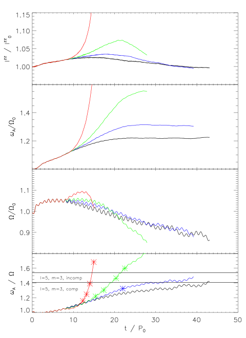
Figure 6: From top to bottom: The moment of inertia $I_{zz}$ of the accretor around the spin axis normalized to its initial value, the mean spin angular velocity of the accretor $\omega_{A}$, the Keplerian estimate of the angular frequency of the binary $\Omega$, and the ratio $\omega_{A}/\Omega$ as functions of time. The angular velocities are referred to the inertial frame and are plotted normalized to the initial binary or corotating frame frequency. The color coding for the curves is the same as in Fig. 4. The bottom frame also shows the two values corresponding to the resonant frequency ratios for the generalized $r$-mode with $l=5$ and $m=3$ for an incompressible spheroid and a polytrope of index $n=3/2$ as deduced from RPA. The asterisks on the curves indicate the approximate times during which accretion belt disturbances resembling modes with (from left to right) $m=6$, 5, 4 and 3 are present (see the movies accompanying Fig. 3). Only $m=6$ is clearly discernible in run Q0.4B.

To summarize, the picture that we have unveiled through these simulations is as follows. Upon reaching contact, the binary is - at least initially - dynamically unstable to mass transfer. This can be expressed with the inequality that $q_{0}>q_{\rm crit}$. The mass transfer rate grows rapidly but the binary then finds a means of escape. The consequential angular momentum loss from the orbit becomes ineffective and angular momentum is returned to the orbit at nearly the same rate that it is advected through the accretion stream. The binary must react as if $q_{\rm crit}=\frac{2}{3}$ and now $q(t)<q_{\rm crit}$. The binary separation expands even faster, the mass transfer rate drops and the dynamical instability is averted.

5 Discussion and Conclusion

We have simulated, hydrodynamically, direct impact accretion in an initially semi-detached, polytropic binary. This model possesses an interesting mass ratio that is intermediate between the two plausible stability bounds of $q_{\rm crit}=\frac{2}{3}$ for very efficient tidal coupling and $q_{\rm crit}\sim 0.2$ that applies when none of the advected angular momentum makes its way back to the orbit. From our baseline evolution we have demonstrated that for this model, $q_{\rm crit}\geq 0.39$ as the mass transfer rate begins to decline once the binary has crossed this mass ratio.

This lower bound for $q_{\rm crit}$ is refined further by evolving the model to its equilibrium mass transfer rate corresponding to an imposed driving loss of angular momentum. From this numerical experiment, we find that $q_{\rm crit}\sim 0.7$, consistent with the expectation for efficient tidal coupling in the binary. This also indicates that the stability boundary itself changes through the evolution. By examining the simulations in light of the individual terms in the orbit-averaged equation for the binary separation (Equation 6), we see that the contribution from the spin-up of the accretor reaches an extreme value and then begins to decline in importance. After the spin of the accretor begins to stabilize, the mass transfer rate begins to decline. We therefore conclude that during the evolution, $q_{\rm crit}$ transitions from the tidally-inefficient to tidally efficient limits on a timescale comparable to the mass-transfer time itself. Although we observe that spin angular momentum is returned to the orbit by tidal coupling to disturbances in the accretion belt, the detailed mechanism by which this is achieved requires further investigation.

The behavior of the Q0.4 model supports the previous simulations we have performed for a DWD binary with an initial mass ratio of $q=0.5$ (DMTF). In that work, we found that the binary expanded and appeared likely to survive intact. However, we were not able to evolve the binary long enough to observe the mass transfer rate declining, though its growth became progressively slower throughout that evolution. We also note that for the DWD binary presented in DMTF, the initial binary components followed the expected mass-radius relation for $n=\frac{3}{2}$ polytropes. At this point, it is important to note that we have examined only two binaries in detail to date and caution is warranted before generalizing our results. This note of caution is especially important for the results presented here for the Q0.4 model. As discussed previously, the accretor is too large compared to the donor star to represent a realistic DWD system and it is plausible that the relative size of the accretor may have exaggerated the efficiency of torques within the binary. To address this concern, we are developing a more flexible SCF code to generate initial data that conform to prescribed ratios for the mass and entropies of the two components. Future simulations, for DWD models with a range of initial mass ratios, will allow us to conclusively map out the effective stability boundaries that hold for binaries undergoing direct impact accretion.

The effective stability bounds that have been discussed here considered only the hydrodynamic flow of material in the self-consistent gravitational potential of the system. In reality, we expect that DWD binaries that begin dynamically unstable mass transfer - and even some systems where the mass transfer remains stable (Han & Webbink (1999); GPF) - accrete at a rate in excess of the Eddington rate. Realistically, we can not neglect the influence of radiation on the dynamics of the accreted material. It is widely expected, though not conclusively demonstrated, that super-Eddington mass transfer will fill a common envelope about the DWD causing the components to inspiral and merge.

To put this statement in a concrete context, in our simulations of the Q0.4 model, the lowest mass transfer rate we can accurately resolve far exceeds the Eddington rate for a white dwarf accretor by 4-5 orders of magnitude. To be consistent, we should really be examining accretion in DWD binaries as a radiative hydrodynamics process. While this goal lies well beyond the scope of the current work, we feel that such simulations may uncover yet more unexpected behavior. For example, the accretion flow from the donor will carry angular momentum that ensures that, at least in the initial phases of the mass transfer, the accreted material will be far from a spherically symmetric state. Radiation from the accretion shock may have a clear channel to escape the system and a common envelope may not even form if the binary can rapidly transition from dynamically unstable to stable mass transfer.

References

- Campbell (1984) Campbell, C.G. 1984, MNRAS, 1984, 433
- D’Souza et al. (2006) D’Souza, M.C., Motl, P.M., Tohline, J.E., & Frank, J. 2006, ApJ 643, 381 (DMTF)
- Gokhale et al. (2007) Gokhale, V., Peng, X.M. & Frank, J. 2007, ApJ 655, 1010, astro-ph/0610919 (GPF)
- Han & Webbink (1999) Han, Z. & Webbink R.F. 1999, A&A, 349, 17
- Hils & Bender (2000) Hils, D. & Bender, P.L. 2000, ApJ 537, 334
- Hils, Bender & Webbink (1990) Hils, D., Bender, P.L. & Webbink, R.F. 1990, ApJ 360, 75
- Marsh et al. (2004) Marsh, T.R., Nelemans, G. & Steeghs, D. 2004, MNRAS, 350, 113
- Motl, Tohline & Frank (2002) Motl, P., Tohline, J.E., & Frank, J. 2002, ApJS 138, 121 (MTF)
- Nelemans, et al. (2001) Nelemans, G., Portegies Zwart, S.F., Verbunt, F. & Yungelson, L.R. 2001, A& A, 368, 939
- Nelemans, Yungelson & Portegies Zwart (2001) Nelemans, G., Yungelson, L. R. & Portegies Zwart, S. F. 2001, A& A 375, 890
- Paczyński (1967) Paczyński, B. 1967, Acta Astr 17, 287
- Postnov & Yungelson (2006) Postnov, K.A. & Yungelson, L.R. 2006, Living Reviews in Relativity, http://www.livingreviews.org/lrr-2006-6
- Racine, Phinney & Arras (2006) Racine, E., Phinney, E.S. & Arras, P. 2006, astro-ph/0610692
- Stone & Norman (1992) Stone,J.M. & Norman, M.L. 1992, ApJS, 80, 753
- Zahn (2005) Zahn, J.-P. 2005, in ASP Conf. Ser. 333, Tidal Evolution and Oscillations in Binary Stars, ed. A. Claret, A. Giménez & J.-P. Zahn (San Francisco: ASP), 4