Propagation of non-WKB Alfvén waves in a multicomponent solar wind with differential ion flow

Abstract

The propagation of dissipationless, hydromagnetic, purely toroidal Alfvén waves in a realistic background three-fluid solar wind with axial symmetry and differential proton-alpha flow is investigated. The short wavelength WKB approximation is not invoked. Instead, the equations that govern the wave transport are derived from standard multi-fluid equations in the five-moment approximation. The Alfvénic point, where the combined poloidal Alfvén Mach number $M_{T}=1$, is found to be a singular point for the wave equation, which is then numerically solved for three representative angular frequencies $\omega=10^{-3}$, $10^{-4}$ and $10^{-5}$ rad s^-1 with a fixed wave amplitude of 10 km s^-1 imposed at the coronal base (1 $R_{\odot}$). The wave energy and energy flux densities as well as wave-induced ion acceleration are computed and compared with those derived in the WKB limit. Between 1 $R_{\odot}$ and 1 AU, the numerical solutions show substantial deviation from the WKB expectations. Even for the relatively high frequency $\omega=10^{-3}$ $\rm rad~{}s^{-1}$, a WKB-like behavior can be seen only in regions $r\gtrsim 10$ $R_{\odot}$. In the low-frequency case $\omega=10^{-5}$ $\rm rad~{}s^{-1}$, the computed profiles of wave-related parameters show a spatial dependence distinct from the WKB one, the deviation being particularly pronounced in interplanetary space. In the inner corona $r\lesssim 4$ $R_{\odot}$, the computed ion velocity fluctuations are considerably smaller than the WKB expectations in all cases, as is the computed wave-induced acceleration exerted on protons or alpha particles. As for the wave energy and energy flux densities, they can be enhanced or depleted compared with the WKB results, depending on $\omega$. With the chosen base wave amplitude, the wave acceleration has negligible effect on the ion force balance in the corona. Hence processes other than the non-WKB wave acceleration are needed to accelerate the ions out of the gravitational potential well of the Sun. However, at large distances beyond the Alfvénic point, the low-frequency waves can play an important role in the ion dynamics, with the net effect being to equalize the speeds of the two ion species considered.

1. INTRODUCTION

Ever since their identification by Belcher & Davis (1971), Alfvén waves have been extensively studied using in situ measurements, such as by Helios and Ulysses, covering the heliocentric distance from 0.29 to 4.3 AU (Tu & Marsch, 1995; Goldstein et al., 1995; Bavassano et al., 2000a, b). On the other hand, the non-thermal broadening of a number of Ultraviolet lines, such as those measured with the SUMER (Solar Ultraviolet Measurements of Emitted Radiation) and UVCS (Ultraviolet Coronagraph Spectrometer) instruments on SOHO (the Solar and Heliospheric Observatory), is usually attributed to the transverse velocity fluctuations, thereby enabling one to infer the amplitudes of these fluctuations in the inner corona below $\sim 5$ $R_{\odot}$ (Banerjee et al., 1998; Esser et al., 1999). Moreover, the Faraday rotation measurements, which yield information regarding the line-of-sight magnetic field fluctuations, have been shown to support indirectly the presence of Alfvén waves inside 10 $R_{\odot}$ (Hollweg et al., 1982). The solar wind in intermediate regions, for the time being, can be explored only by radio scintillation measurements which allow one to derive the velocity fluctuations (e.g., Armstrong & Woo, 1981; Scott et al., 1983). It is noteworthy that although the hourly-scale fluctuations seem to be more frequently studied, the fluctuation spectrum measured by Helios nevertheless spans a broad frequency range from $10^{-5}$ to $10^{-2}$ $\rm s^{-1}$ (Tu & Marsch, 1995).

Most of the theoretical investigations into the interaction between Alfvén waves and the solar wind have been performed in the short wavelength WKB limit which makes the problem more tractable mathematically. For instance, by employing the WKB approximation, Parker (1965) derived an expression for the ponderomotive force through which the Alfvén waves may provide further acceleration to the solar wind. The wave acceleration was later incorporated in detailed numerical models by, e.g., Alazraki & Couturier (1971). It was soon realized that Alfvén waves may also heat the solar wind via dissipative processes such as the cyclotron resonance interaction between ions and high frequency, parallel propagating waves generated by a turbulent cascade (cf. the extensive review by Hollweg & Isenberg (2002)). Such a parallel cascade scenario has been successful in explaining a number of observations, to name but one, the significant thermal anisotropy of ions as established by UVCS measurements (Li et al., 1999). As pointed out by Hollweg & Isenberg (2002), the applicability of the WKB approximation in which the processes are formulated is questionable in the near-Sun region in view of the large Alfvén speeds. Furthermore, a turbulent cascade requires a non-vanishing magnetic Reynolds stress tensor, which, however, is zero in the WKB limit since the particle and field components of the tensor cancel each other exactly. A non-WKB analysis is therefore required to account for the wave reflection and the consequent driving of any turbulence cascade.

As a matter of fact, non-WKB analysis of Alfvén waves in the solar wind has been carried out for decades (e.g., Heinemann & Olbert, 1980; Lou, 1993). This, however, is almost exclusively done in the framework of ideal MHD, which allows waves propagating in opposite directions to be explicitly separated when the Elsässer variables are used. The adoption of the Elsässer variables has also enabled a new turbulence phenomenology concerning the nonlinear coupling between counter-propagating waves (Dmitruk et al., 2001; Cranmer & van Ballegooijen, 2005; Verdini et al., 2005). This coupling term, if interpreted as the energy cascaded towards fluctuations with increasingly large perpendicular wavenumbers, is also more consistent with theoretical expectations.

Despite substantial advances achieved in ideal MHD, which is appropriate for the description of the gross properties of the solar wind, the non-WKB analysis of Alfvén waves has rarely been done using multi-fluid transport equations. In contrast, multi-fluid, Alfvén wave driven solar wind modeling formulated in the WKB limit has reached considerable sophistication (see Hollweg & Isenberg, 2002). Such a multi-fluid approach is particularly necessary for the solar wind since the alpha particles must be included given their non-negligible abundance and the fact that the proton-alpha differential speed can be a substantial fraction of the proton speed in the fast stream (Marsch et al., 1982). There is therefore an obvious need to extend available non-WKB analyses of Alfvén waves from the ideal MHD to the multi-fluid case.

The intent of this paper is to present an analysis of Alfvén waves in a 3-fluid solar wind assuming axial symmetry, without assuming that the wavelength is small compared with the spatial scales at which the background parameters vary. The perturbed velocity and magnetic field are assumed to be in the azimuthal direction, i.e, only purely toroidal waves are investigated. To further simplify the treatment, the wave dissipation is neglected. This simplification is necessary here since if one wants to gain some quantitative insights into the wave dissipation, and to maintain a reasonable self-consistency at the same time, one should formulate the dissipation in terms of the amplitudes of waves propagating outwards and inwards. To this end, a full multi-fluid Elsässer analysis is required but is unfortunately unavailable at the present time. However, if the wave dissipation is neglected and therefore the nonlinear interaction between waves and the multicomponent wind is entirely through the agent of ponderomotive forces, then the problem can be formulated without distinguishing explicitly between the directions of wave propagation (cf. Lou, 1993).

The paper is organized as follows. In section 2, we show how to reduce the general multi-fluid transport equations to the desired form. The resultant equations governing the Fourier amplitudes of toroidal Alfvén waves at a given frequency are then solved analytically in two limiting cases, namely the WKB and zero-frequency limits, in section 3. Apart from these analytically tractable cases, the equations have to be solved numerically. In section 4, we re-formulate the model equations for numerical convenience, describe the background flow parameters and detail the solution procedure as well. The numerical solutions for three different frequencies are presented in section 5. Finally, section 6 summarizes the results, ending with some concluding remarks.

2. MATHEMATICAL FORMULATION

Presented in this section is the mathematical development of the equations that govern the toroidal fluctuations in a solar wind which consists of electrons ($e$), protons ($p$) and alpha particles ($\alpha$). Each species $s$ ($s=e,p,\alpha$) is characterized by its mass $m_{s}$, electric charge $e_{s}$, number density $n_{s}$, mass density $\rho_{s}=n_{s}m_{s}$, velocity $\mathbf{v}_{s}$, and partial pressure $p_{s}$. If measured in units of the electron charge $e$, $e_{s}$ may be expressed by $e_{s}=Z_{s}e$ with $Z_{e}\equiv-1$ by definition.

To simplify the mathematical treatment, a number of assumptions have been made and are collected as follows:

1. It is assumed that the solar wind can be described by the standard transport equations in the five-moment approximation.

2. Quasi neutrality and quasi-zero current are assumed, i.e., $n_{e}=\sum_{k}Z_{k}n_{k}$ and $\mathbf{v}_{e}=\sum_{k}Z_{k}n_{k}\mathbf{v}_{k}/n_{e}$ where $k=p,\alpha$.

3. Symmetry about the magnetic axis is assumed, i.e., $\partial/\partial\phi\equiv 0$ in a heliocentric spherical coordinate system ($r,\theta,\phi$).

4. The time-independent solar wind interacts with the waves only through the wave-induced ponderomotive forces.

5. The wave frequency considered is in the hydromagnetic regime, i.e., well below the ion gyro-frequencies.

6. The perturbed velocity and magnetic field are assumed to be in the $\phi$ direction only.

7. The effects of the solar rotation on the background solar wind are neglected such that there is no need to consider the coupling of Alfvén waves to the compressional modes in the presence of a spiral magnetic field.

8. The effects of the Coulomb friction on the waves are neglected, and so is the wave-induced modification of the Coulomb friction between background ion flows.

2.1. Multi-fluid Equations

The equations appropriate for a multi-component solar wind plasma in the standard five-moment approximation are as follows (for the derivation see appendix A.1 in Li & Li (2006))

$$\frac{\partial n_{k}}{\partial t} + \nabla\cdot(n_{k}\mathbf{v}_{k})=0,$$ (1)

$$\frac{\partial\mathbf{v}_{k}}{\partial t} + \mathbf{v}_{k}\cdot\nabla\mathbf{v}_{k}+\frac{\nabla p_{k}}{n_{k}m_{k}}+\frac{Z_{k}\nabla p_{e}}{n_{e}m_{k}}+\frac{GM_{\odot}}{r^{2}}\hat{r}$$ (2)

$$- \frac{1}{n_{k}m_{k}}\left[\frac{\delta\mathbf{M}_{k}}{\delta t}+\frac{Z_{k}n_{k}}{n_{e}}\frac{\delta\mathbf{M}_{e}}{\delta t}\right]$$

$$- \frac{Z_{k}}{4\pi n_{e}m_{k}}\left(\nabla\times\mathbf{B}\right)\times\mathbf{B}$$

$$+ \frac{Z_{k}e}{m_{k}c}\frac{n_{j}Z_{j}}{n_{e}}\left(\mathbf{v}_{j}-\mathbf{v}_{k}\right)\times\mathbf{B}=0,$$

$$\frac{\partial}{\partial t}\frac{p_{s}}{\gamma-1} + \mathbf{v}_{s}\cdot\nabla\frac{p_{s}}{\gamma-1}+\frac{\gamma}{\gamma-1}p_{s}(\nabla\cdot\mathbf{v}_{s})$$ (3)

$$+ \nabla\cdot\mathbf{q}_{s}-\frac{\delta E_{s}}{\delta t}-Q_{s}=0,$$

$$\frac{\partial\mathbf{B}}{\partial t} - \nabla\times\left(\mathbf{v}_{e}\times\mathbf{B}\right)=0,$$ (4)

where the subscript $s$ refers to all species ($s=e,p,\alpha$), while $k$ stands for ion species only ($k=p,\alpha$). The gravitational constant is denoted by $G$, $M_{\odot}$ is the mass of the Sun, $\mathbf{B}$ the magnetic field and $c$ the speed of light. The momentum and energy exchange rates due to the Coulomb collisions of species $s$ with the remaining ones are denoted by $\delta\mathbf{M}_{s}/\delta t$ and $\delta E_{s}/\delta t$, respectively. Moreover, $\mathbf{q}_{s}$ is the heat flux carried by species $s$, and $Q_{s}$ stands for the heating rate applied to species $s$ from non-thermal processes. In equation (2), the subscript $j$ stands for ion species other than $k$, namely, $j=p$ for $k=\alpha$ and vice versa. As can be seen, in addition to the term $(\nabla\times\mathbf{B})\times\mathbf{B}$, the Lorentz force possesses a new term in the form of the cross product of the ion velocity difference and magnetic field. Physically, this new term represents the mutual gyration of one ion species about the other, the axis of gyration being in the direction of the instantaneous magnetic field.

Equations (1) to (4) form a complete set if supplemented with the description of species heat fluxes $\mathbf{q}_{s}$ and heating rates $Q_{s}$. As such, they can be invoked to depict self-consistently the interaction between Alfvén waves and the solar wind species by explicitly introducing these waves via boundary conditions. On the one hand solving this set of equations presents a computationally formidable task; on the other hand, one can extract the necessary information concerning the dynamical feedback of the waves to the plasma by going beyond the WKB limit. In the non-WKB approach to be adopted here, one assumes that the governing equations can still be separated into those governing the background time-independent flow and those governing the transport of waves. As noted by Lou (1993) (also see the discussion), this separation does not necessarily require the waves be linear as long as sufficiently small wave amplitudes are imposed at the Sun.

Further simplification also results from the choice of a flux tube coordinate system, in which the base vectors are $\{\hat{e}_{l},\hat{e}_{N},\hat{e}_{\phi}\}$, where

$$\hat{e}_{l}=\mathbf{B}_{P}/B_{P},\hskip 14.22636pt\hat{e}_{N}=\hat{e}_{\phi}\times\hat{e}_{l},$$

with the subscript $P$ denoting the poloidal component. Moreover, the independent variable $l$ is the arclength along the poloidal magnetic field line. This choice permits the decomposition of the magnetic field and species velocities into background ones and fluctuations,

$$\mathbf{B}=B_{l}\hat{e}_{l}+b\hat{e}_{\phi},\hskip 14.22636pt\mathbf{v}_{s}=U_{s}\hat{e}_{l}+w_{s}\hat{e}_{N}+u_{s}\hat{e}_{\phi}.$$ (5)

where $s=e,p,\alpha$. From the assumption of azimuthal symmetry, and the assumption that $\mathbf{B}_{P}$ is time-independent, one can see from the poloidal component of equation (4) that $\mathbf{v}_{eP}$ should be strictly in the direction of $\mathbf{B}_{P}$. In other words, $w_{e}=0$ to a good approximation. Now let us consider the $\phi$ component of the momentum equation (2). Since the wave frequencies in question as well as other frequencies associated with the spatial dependence are well below the ion gyro-frequency $\Omega_{k}=(Z_{k}eB_{l})/(m_{k}c)$ ($k=p,\alpha$), from an order-of-magnitude estimate one can see that $|w_{j}-w_{k}|\ll|u_{k}|$. Combined with the fact that $w_{e}=0$, this leads to that both $w_{p}$ and $w_{\alpha}$ should be very small and can be safely neglected unless they appear alongside the ion gyro-frequency. With this in mind, one can find from the $N$ component of equation (2) that

$$u_{\alpha}-u_{p}=\frac{b}{B_{l}}\left(U_{\alpha}-U_{p}\right).$$ (6)

That is, the ion velocity difference is aligned with the instantaneous magnetic field. This alignment condition further couples one ion species to the other. Note that due to the assumption of quasi-zero current, equation (6) leads to

$$u_{k}=u_{e}+\frac{b}{B_{l}}\left(U_{k}-U_{e}\right)$$ (7)

where $k=p,\alpha$.

Given the aforementioned assumptions, the time-independent multicomponent solar wind in which the toroidal Alfvén waves propagate is governed by

$$B_{l}\left(\frac{n_{k}U_{k}}{B_{l}}\right)^{\prime}=0,$$ (8)

$$U_{k}U_{k}^{\prime}+\frac{p_{k}^{\prime}}{n_{k}m_{k}}+\frac{Z_{k}p_{e}^{\prime}}{n_{e}m_{k}}+\frac{GM_{\odot}}{r}(\ln r)^{\prime}$$

$$-\frac{1}{n_{k}m_{k}}\left(\frac{\delta M_{kl}}{\delta t}+\frac{Z_{k}n_{k}}{n_{e}}\frac{\delta M_{el}}{\delta t}\right)=a_{w,k},$$ (9)

$$U_{s}\left(\frac{p_{s}}{\gamma-1}\right)^{\prime}+\frac{\gamma p_{s}}{(\gamma-1)}B_{l}\left(\frac{U_{s}}{B_{l}}\right)^{\prime}$$

$$+B_{l}\left(\frac{q_{s}}{B_{l}}\right)^{\prime}-\frac{\delta E_{s}}{\delta t}-Q_{s}=0,$$ (10)

where the prime denotes the derivative with respect to the arclength $l$ which becomes the only independent spatial variable. In addition, $a_{w,k}$ denotes the acceleration exerted on ion species $k$ ($k=p,\alpha$) by the toroidal fluctuations,

$$a_{w,k} = \left<u_{k}^{2}\right>(\ln R)^{\prime}-\frac{Z_{k}}{4\pi n_{e}m_{k}}\left<b\frac{\partial b}{\partial l}+b^{2}(\ln R)^{\prime}\right>$$ (11)

$$- \frac{\left<bX_{k}\right>}{B_{l}},$$

where $R=r\sin\theta$ is the distance from a point along the poloidal magnetic field line to the magnetic axis. Besides, the angular brackets stand for the time-average over one wave period. The variable $X_{k}=\Omega_{k}(w_{j}-w_{k})(Z_{j}n_{j}/n_{e})$ distinguishes the present study from those using the ideal MHD in which case $X_{k}\equiv 0$ (e.g., Heinemann & Olbert, 1980). Apart from this, the wave-induced acceleration $a_{w,k}$ includes the inertial centrifugal acceleration (the first term on the right hand side), and the usual $(\nabla\times\mathbf{B})\times\mathbf{B}$ term (the second term).

2.2. Transport of Toroidal Alfvén Waves

The transport of toroidal Alfvén waves is governed by the azimuthal component of the momentum equation (2) for ion species $k$ ($k=p,\alpha$) together with that of the magnetic induction law (4). To be more specific, these equations read

$$\frac{\partial b}{\partial t} + B_{l}R\frac{\partial}{\partial l}\left[\frac{1}{R}\left(\frac{U_{e}}{B_{l}}b-u_{e}\right)\right]=0,$$ (12)

$$\frac{\partial u_{k}}{\partial t} + U_{k}\left[\frac{\partial u_{k}}{\partial l}+u_{k}(\ln R)^{\prime}\right]$$ (13)

$$- \frac{Z_{k}}{4\pi n_{e}m_{k}}B_{l}\left[\frac{\partial b}{\partial l}+b(\ln R)^{\prime}\right]=X_{k}.$$

The wave propagation is characterized by several key parameters, namely, the wave energy and energy flux densities as well as the wave-induced acceleration. These parameters can be found by considering the energy conservation for the Alfvén waves,

$$\frac{\partial}{\partial t}(\sum_{k}\frac{\rho_{k}u_{k}^{2}}{2}+\frac{b^{2}}{8\pi})+B_{l}\frac{\partial}{\partial l}\left\{\frac{1}{B_{l}}\left[\sum_{k}\frac{\rho_{k}U_{k}u_{k}^{2}}{2}\right.\right.$$ (14)

$$+ \left.\left.\frac{b}{4\pi}\left(U_{e}b-B_{l}u_{e}\right)\right]\right\}$$

$$= -\sum_{k}\rho_{k}U_{k}u_{k}^{2}(\ln R)^{\prime}+\frac{U_{e}}{4\pi}\left[b\frac{\partial}{\partial l}b+b^{2}(\ln R)^{\prime}\right]$$

$$+\sum_{k}\rho_{k}u_{k}X_{k}.$$

On the left hand side (LHS), the first term is the time derivative of the perturbation energy density, while the second is the divergence of the perturbation flux density. The physical meaning of the right hand side (RHS) can be revealed as follows. By using relation (7) one finds

$$\sum_{k}\rho_{k}u_{k}X_{k}-\sum_{k}\rho_{k}U_{k}\frac{bX_{k}}{B_{l}}=\left(u_{e}-\frac{b}{B_{l}}U_{e}\right)\sum_{k}\rho_{k}X_{k}.$$

Since $\sum_{k}\rho_{k}X_{k}=0$, one can identify the time-average of the RHS of equation (14) as the negative of the work done by the wave-induced forces on the solar wind, i.e., $\sum_{k}\rho_{k}U_{k}a_{w,k}$ (cf. Eq.(11)). In other words, taking the time-average of equation (14) yields

$$B_{l}\frac{\partial}{\partial l}\frac{F_{w}}{B_{l}}=-\sum_{k}\rho_{k}U_{k}a_{w,k},$$ (15)

where $F_{w}$ is the time-average of the perturbation flux density and will be termed wave flux density for simplicity. (Actually, the wave properties to be discussed always refer to time-averaged values.) The total energy is therefore conserved for the system comprised of a multi-fluid solar wind and toroidal Alfvén waves: The gain in the solar wind kinetic energies is at the expense of the wave energy.

The appearance of $X_{k}$ makes equation (13) inconvenient to work with. Instead one may consider the azimuthal component of the total momentum to eliminate $X_{k}$, the resultant equation being

$$\sum_{k}\rho_{k}\left[\frac{\partial u_{k}}{\partial t}+\frac{U_{k}}{R}\frac{\partial}{\partial l}\left(Ru_{k}\right)\right]$$ (16)

$$- \frac{B_{l}}{4\pi R}\frac{\partial}{\partial l}\left(Rb\right)=0.$$

Now one may proceed by introducing the Fourier amplitudes at a given angular frequency $\omega$,

$$[b(l,t),u_{s}(l,t)]=[\tilde{b}(l),\tilde{u}_{s}(l)]\exp(-i\omega t),$$ (17)

in which $s=e,p,\alpha$. As a result, the Faraday’s law (12) and equation (16) now take the form

$$U_{e}\tilde{b}^{\prime}-B_{l}\tilde{u}_{e}^{\prime}$$

$$= \left[i\omega+U_{e}\left(\ln\frac{RB_{l}}{U_{e}}\right)^{\prime}\right]\tilde{b}-B_{l}(\ln R)^{\prime}\tilde{u}_{e},$$

$$\left(\sum_{k}\rho_{k}U_{k}\frac{U_{k}-U_{e}}{B_{l}}-\frac{B_{l}}{4\pi}\right)\tilde{b}^{\prime}+\sum_{k}\rho_{k}U_{k}\tilde{u}_{e}^{\prime}$$

$$= -\left[\sum_{k}\frac{\rho_{k}U_{k}}{R}\left(R\frac{U_{k}-U_{e}}{B_{l}}\right)^{\prime}-\frac{B_{l}}{4\pi}\left(\ln R\right)^{\prime}\right]\tilde{b}$$

$$- \sum_{k}\rho_{k}U_{k}\left(\ln R\right)^{\prime}\tilde{u}_{e}$$

$$+ i\omega\sum_{k}\rho_{k}\left(\frac{U_{k}-U_{e}}{B_{l}}\tilde{b}+\tilde{u}_{e}\right),$$ (19)

in which we have used relation (7) to express the ion velocity fluctuation $\tilde{u}_{k}$ in terms of the electron one $\tilde{u}_{e}$.

Once the background flow parameters and proper boundary conditions are given, equations (2.2) and (19) can be solved for the Fourier amplitudes of magnetic fluctuation $\tilde{b}$ and the electron velocity fluctuation $\tilde{u}_{e}$ for a given angular frequency $\omega$. The ion velocity fluctuations $\tilde{u}_{k}$ can then be found in virtue of relation (7). The three wave-related parameters can be evaluated by forming a time-average over one wave period. Specifically, the wave energy density $E_{w}$ and wave energy flux density $F_{w}$ are given by

$$E_{w} = \sum_{k}\frac{\rho_{k}\left<u_{k}^{2}\right>}{2}+\frac{\left<b^{2}\right>}{8\pi},$$ (20a)

$$F_{w} = \sum_{k}\frac{\rho_{k}U_{k}\left<u_{k}^{2}\right>}{2}$$ (20b)

$$+ \frac{1}{4\pi}\left(U_{e}\left<b^{2}\right>-B_{l}\left<bu_{e}\right>\right),$$

while the wave-induced acceleration $a_{w,k}$ has already been given by equation (11). It can be seen that $E_{w}$ consists of the ion kinetic as well as the magnetic energies, while $F_{w}$ is comprised of the kinetic energy flux convected by ion fluids and the Poynting flux. To evaluate the time-average $\left<fg\right>$ for two wave-related fluctuations $[f,g]\sim[\tilde{f},\tilde{g}]\exp(-i\omega t)$, one may use the expression (cf. MacGregor & Charbonneau, 1994)

$$\left<fg\right>=\frac{1}{2}\mathrm{Re}(\tilde{f}\tilde{g}^{*})=\frac{1}{4}(\tilde{f}\tilde{g}^{*}+\tilde{f}^{*}\tilde{g}),$$ (21)

where $\mathrm{Re}(z)$ denotes the real part of a complex variable $z$, and the superscript asterisk denotes the complex conjugate.

Although in general one has to rely on a numerical integrator to solve equations (2.2) and (19), as shown below, they are analytically tractable for two limiting cases.

3. ANALYTICAL SOLUTIONS IN TWO LIMITS

In this section, we will examine the analytical solutions to equations (2.2) and (19) in the WKB and zero-frequency ($\omega=0$) limits. These analytical treatments not only help to validate numerical solutions, but also allow one to gain insights into the mathematical properties of the governing equations.

3.1. the WKB Limit

Extensive studies have been made on the Alfvén waves in the WKB limit. In particular, the Alfvén wave force exerted on differentially streaming ions was first derived by Hollweg (1974) and later by McKenzie et al. (1979) for a spherically expanding solar wind. Based on the idea of the wave average Lagrangian, the work by Isenberg & Hollweg (1982) not only obtained the expression for the wave force but further showed that there exists an adiabatic invariant, namely the wave action flux, in the absence of wave dissipation. The derivation is rather general and does not require a specific flux tube geometry. Alternatively, the action flux conservation has been independently obtained by McKenzie (1994) who used the more familiar WKB analysis. Although McKenzie (1994) assumed that the solar wind is again spherically symmetric, his results can be readily extended to an axisymmetric configuration. In what follows, such an extension is presented.

The formal development of the WKB analysis starts with the introduction of the expansion

$$\tilde{u}_{s}=(u_{s,1}+u_{s,2}+\cdots)\exp(iS(l)),$$ (22a)

$$\tilde{b}=(b_{1}+b_{2}+\cdots)\exp(iS(l)),$$ (22b)

in which $s=e,p,\alpha$. It is assumed that $u_{s,n}$ and $b_{n}$ ($n=1,2,...$) vary at the same spatial scale $H$ as the background flow parameters, and $1/H$ is small compared with the wave number $K=S^{\prime}(l)$, i.e., $\mu=1/(KH)\ll 1$. In addition, it is assumed that $|u_{s,n+1}/u_{s,n}|\sim|b_{n+1}/b_{n}|\sim\mu$. Substituting the expansion (3.1) into equations (2.2) and (19), one can find by sorting different terms according to orders of $\mu$ that

$$\omega_{e}b_{n}+KB_{l}u_{e,n}$$

$$= -iRB_{l}\left[\frac{1}{R}\left(\frac{U_{e}}{B_{l}}b_{n-1}-u_{e,n-1}\right)\right]^{\prime},$$

$$\sum_{k}\rho_{k}\omega_{k}\left(u_{e,n}+\frac{U_{k}-U_{e}}{B_{l}}b_{n}\right)+K\frac{B_{l}}{4\pi}b_{n}$$

$$= -i\sum_{k}\frac{\rho_{k}U_{k}}{R}\left[R\left(u_{e,n-1}+\frac{U_{k}-U_{e}}{B_{l}}b_{n-1}\right)\right]^{\prime}$$

$$+ i\frac{B_{l}}{4\pi R}\left(Rb_{n-1}\right)^{\prime},$$ (23b)

where the definition $\omega_{s}=\omega-KU_{s}$ ($s=e,p,\alpha$) has been used.

At the lowest order $n=1$, the RHS of equation (3.1) is zero. For $u_{e,1}$ and $b_{1}$ not to be identically zero, the determinant of the coefficient matrix has to be zero. As a result, one finds the local dispersion relation

$$\sum_{k}\rho_{k}(U_{ph}-U_{k})^{2}=\frac{B_{l}^{2}}{4\pi},$$ (24)

where $U_{ph}=\omega/K$ is the local phase speed of Alfvén waves. Furthermore, one can find the local eigen-relations at order $n=1$,

$$u_{s,1}=-\left(U_{ph}-U_{s}\right)\frac{b_{1}}{B_{l}},$$ (25)

with $s=e,p,\alpha$.

At an arbitrary order $n\geq 2$, it follows from equation (3.1) that

$$u_{e,n}=-\left(U_{ph}-U_{e}\right)\frac{b_{n}}{B_{l}}+\bar{u}_{n},$$

in which

$$\bar{u}_{n}=-\frac{iR}{K}\left[\frac{1}{R}\left(\frac{U_{e}}{B_{l}}b_{n-1}-u_{e,n-1}\right)\right]^{\prime}$$

arises from quantities at order $n-1$. At order $n+1$, one can eliminate $b_{n+1}$ and $u_{e,n+1}$ on the LHS of equation (3.1) by using the dispersion relation (24), the resultant equations taking the form

$$T_{n}+S_{n} = 0,$$ (26)

where

$$S_{n} = -\left[\sum_{k}\rho_{k}\omega_{k}RB_{l}\left(\frac{\bar{u}_{n}}{R}\right)^{\prime}\right.$$ (27a)

$$+ \left.KB_{l}\sum_{k}\frac{\rho_{k}U_{k}}{R}\left(R\bar{u}_{n}\right)^{\prime}\right],$$

$$T_{n} = \sum_{k}\rho_{k}\omega_{k}RB_{l}\left(\frac{U_{ph}b_{n}}{RB_{l}}\right)^{\prime}$$ (27b)

$$+ KB_{l}\sum_{k}\frac{\rho_{k}U_{k}}{R}\left(R\frac{U_{ph}-U_{k}}{B_{l}}b_{n}\right)^{\prime}$$

$$+ K\frac{B_{l}^{2}}{4\pi R}\left(Rb_{n}\right)^{\prime}.$$

The barred and unbarred parts are again distinguished.

On expanding $T_{n}$, by repeatedly using the dispersion relation (24) one finds that

$$T_{n}=\frac{KB_{l}^{3}}{U_{ph}b_{n}}\left[\left(\frac{U_{ph}b_{n}}{B_{l}}\right)^{2}\frac{\rho(U_{ph}-U_{m})}{B_{l}}\right]^{\prime},$$ (28)

in which the following definitions have been used (cf. McKenzie, 1994)

$$\rho=\sum_{k}\rho_{k},$$ (29a)

$$\rho U_{m}=\sum_{k}\rho_{k}U_{k},$$ (29b)

$$\rho U_{j}^{2}=\sum\rho_{k}U_{k}^{2},$$ (29c)

with the last one defined for future use. If putting $n=1$, from $S_{1}=0$ one finds $T_{1}=0$, i.e.,

$$b_{1}^{2}\frac{\rho(U_{ph}-U_{m})U_{ph}^{2}}{B_{l}^{3}}=\mbox{const}.$$ (30)

Note that equation (30) can be interpreted in terms of the conservation of wave action flux, which was first found by Isenberg & Hollweg (1982). On the other hand, expanding equation (13) to first order in $\mu$ and using the resultant $X_{k}$ to evaluate $\left<bX_{k}\right>$ in equation (11), with the aid of the eigen-relation (25), one can find a compact expression for the wave-induced acceleration on ion species $k$ ($k=p,\alpha$),

$$a_{w,k}=\left(\frac{U_{ph}^{2}-U_{k}^{2}}{2B_{l}^{2}}\left<b^{2}\right>\right)^{\prime},$$ (31)

where the time-average $\left<b^{2}\right>=|b_{1}|^{2}/2$. It is noteworthy that the shape of the line of force, which enters into the discussion through $R=r\sin\theta$, does not show up via $S_{n-1}$ unless one examines the evolution of higher order fluctuations $u_{s,n}$ and $b_{n}$ ($n\geq 2$).

Some remarks on the wave acceleration $a_{w,k}$ given by Equation (31) are necessary. One may find that $(U_{\alpha}^{2}-U_{p}^{2})(1+|b_{1}|^{2}/(2B_{l}^{2}))=\mbox{const}$ if the flow speeds are entirely determined by the wave forces. Usually $|b_{1}|/B_{l}$ increases with increasing distance. The net effect of $a_{w,k}$ is therefore to limit the proton-alpha differential speed $U_{\alpha p}$. In this sense $a_{w,k}$ was likened to an additional frictional force (e.g., Hollweg, 1974). As noted by Hollweg (1974), the differential nature of $a_{w,k}$ derives eventually from a wave-induced transverse drift velocity $\delta\mathbf{u}_{k}$ ($k=p,\alpha$), which is different for different species because they see different wave electric fields when they flow differentially. The contribution to the wave force from $\delta\mathbf{u}_{k}$ is twofold. First, it induces a centrifugal force that is always non-negative. Second, it contributes to the species electric current flow $\delta\mathbf{J}_{\perp,k}$ which in turn exerts on ion species $k$ a $\delta\mathbf{J}_{\perp,k}\times\delta\mathbf{B}$ force, where $\delta\mathbf{B}$ is the wave magnetic field. This force may become negative. As a matter of fact, the two terms may even add up to a negative value: The wave force may decelerate rather than accelerate the ion species. Consider a simplified situation similar to that considered by Hollweg (1974). One assumes that the spatial variation of both $U_{\alpha}$ and $U_{p}$ can be neglected, and $U_{\alpha}>U_{p}>U_{A}$ where $U_{A}=B_{l}/\sqrt{4\pi\rho}$ is the bulk Alfvén speed. One may further assume that the alpha particles are test particles, the background magnetic field is purely radial, and that $|b_{1}|^{2}\propto r^{-\epsilon}$ with $\epsilon$ being a positive constant. In this case, from Equation (31) one finds that

$$a_{w,\alpha}=\frac{|b_{1}|^{2}}{4B_{l}^{2}r}\left\{\left[\left(4-\epsilon\right)U_{p}^{2}+\epsilon U_{A}^{2}\right]-\left(4-\epsilon\right)\left(U_{\alpha p}+U_{p}\right)^{2}\right\}.$$

It follows that $a_{w,\alpha}<0$ when $U_{\alpha p}>U_{c}$ where the critical value $U_{c}$ can be roughly approximated by

$$U_{c}\approx\frac{\epsilon}{2(4-\epsilon)}\frac{U_{A}}{U_{p}}U_{A},$$

which may be smaller than $U_{A}$ by a factor of ${U_{A}}/{U_{p}}$. Noting that now the wave phase speed is $U_{ph}=U_{p}+U_{A}$, one finds that the waves may decelerate alpha particles even though $U_{\alpha}<U_{ph}$. It turns out that this much simplified picture roughly represents the behavior of $a_{w,\alpha}$ in the region between 20 and 30 $R_{\odot}$ where $\epsilon$ can be taken to be $2.5$ for the adopted background flow parameters (see Figure 5b which indicates that $a_{w,\alpha}$ in the WKB case becomes negative beyond 22.7 $R_{\odot}$ where $U_{\alpha p}$ exceeds $U_{c}$).

3.2. the Zero-frequency Limit

The other extreme will be $\omega=0$. In this case, equations (12) and (16) can be integrated to yield

$$u_{e}-U_{e}\frac{b}{B_{l}}=A_{\Omega}R,$$ (32a)

$$R\left[\sum_{k}\frac{\rho_{k}U_{k}}{\rho U_{m}}u_{k}-\frac{B_{l}b}{4\pi\rho U_{m}}\right]=A_{L},$$ (32b)

where $A_{\Omega}$ and $A_{L}$ are two integration constants. When deriving equation (32b), we have used the fact that $\rho U_{m}/B_{l}$ is a constant. Equation (3.2) demonstrates a clear connection to the problem of angular momentum transport in a multicomponent solar wind, as has been discussed by Li & Li (2006).

With the aid of equation (7), equation (3.2) can be solved to yield

$$b=R\frac{4\pi\rho U_{m}}{B_{l}}\frac{A_{L}/R^{2}-A_{\Omega}}{M_{T}^{2}-1},$$ (33)

where

$$M_{T}^{2}=\frac{4\pi\rho U_{j}^{2}}{B_{l}^{2}}$$ (34)

is the square of the combined Alfvén Mach number. For typical solar winds, there exists one point where $M_{T}=1$ between 1 $R_{\odot}$ and 1 AU. Call this point the Alfvénic point, and let it be denoted by subscript $A$. It then follows that for $b$ not to be singular at this point, one must require $A_{L}=A_{\Omega}R_{A}^{2}$. As a result, one may obtain

$$b= A_{\Omega}R\frac{4\pi\rho U_{m}}{B_{l}}\frac{(R_{A}/R)^{2}-1}{M_{T}^{2}-1},$$ (35a)

$$u_{s}= A_{\Omega}R\left[1+\frac{4\pi\rho U_{m}U_{s}}{B_{l}^{2}}\frac{(R_{A}/R)^{2}-1}{M_{T}^{2}-1}\right],$$ (35b)

where $s=e,p,\alpha$.

4. NUMERICAL MODEL AND METHOD OF SOLUTION

Apart from the WKB and zero-frequency limits, equations (2.2) and (19) can be integrated only numerically. Nevertheless, the treatment in the zero-frequency limit in the previous section reveals that the Alfvénic point where $M_{T}^{2}=1$ is a singular point for the system of equations. One may expect that this is also the case for an arbitrary finite $\omega$. In their present form, however, equations (2.2) and (19) do not show explicitly the existence of such a singular point. Hence they are not convenient to work with numerically and need to be further developed in what follows. Moreover, we will also describe how to specify the background flow parameters, and the solution procedure as well.

4.1. Further Development of Governing Equations

For the convenience of presentation, one may define, in addition to $M_{T}$, the following dimensionless parameters

$$X_{me}=\frac{4\pi\rho U_{m}U_{e}}{B_{l}^{2}},X_{ee}=\frac{4\pi\rho U_{e}U_{e}}{B_{l}^{2}},$$

$$X_{eA}=\frac{4\pi\rho U_{e}U_{A}}{B_{l}^{2}},X_{mA}=\frac{4\pi\rho U_{m}U_{A}}{B_{l}^{2}},$$

$$Z=M_{T}^{2}-1-X_{me},$$ (36)

in which $U_{A}=B_{l}/\sqrt{4\pi\rho}$ is the bulk Alfvén speed. Now equation (19) can be expressed as

$$Z\tilde{b}^{\prime} + \frac{4\pi\rho U_{m}}{B_{l}}\tilde{u}_{e}^{\prime}=-\frac{(RZ)^{\prime}}{R}\tilde{b}-\frac{4\pi\rho U_{m}(\ln R)^{\prime}}{B_{l}}\tilde{u}_{e}$$ (37)

$$+i\omega\left(\frac{4\pi\rho(U_{m}-U_{e})}{B_{l}^{2}}\tilde{b}+\frac{4\pi\rho}{B_{l}}\tilde{u}_{e}\right).$$

Taking into account equation (2.2), one finally arrives at

$$\left(M_{T}^{2}-1\right){\xi}^{\prime} = F_{11}\xi+F_{12}\eta,$$ (38a)

$$\left(M_{T}^{2}-1\right){\eta}^{\prime} = F_{21}\xi+F_{22}\eta,$$ (38b)

where two dimensionless variables have been introduced for convenience,

$$\xi=\tilde{b}/B_{l},\hskip 11.38092pt\eta=\tilde{u}_{e}/U_{A}.$$ (39)

Moreover, the coefficients are

$$F_{11} = \frac{i\omega}{U_{e}}\left(2X_{me}-X_{ee}\right)+X_{me}\left(\ln\frac{R}{U_{e}}\right)^{\prime}$$ (40a)

$$-\frac{(RB_{l}Z)^{\prime}}{RB_{l}}$$

$$F_{12} = \frac{i\omega}{U_{e}}X_{eA}-2X_{mA}\left(\ln R\right)^{\prime}$$ (40b)

$$F_{21} = -\frac{i\omega}{U_{A}}\left(Z-X_{me}+X_{ee}\right)$$ (40c)

$$- \frac{U_{e}}{U_{A}}\left[Z\left(\ln\frac{RB_{l}}{U_{e}}\right)^{\prime}+\frac{(RZ)^{\prime}}{R}\right]$$

$$F_{22} = \frac{i\omega}{U_{e}}X_{ee}+\left(Z-X_{me}\right)\left(\ln R\right)^{\prime}$$ (40d)

$$- (M_{T}^{2}-1)(\ln U_{A})^{\prime}.$$

It is now clear that the Alfvénic point where $M_{T}^{2}=1$ is a singular point for equation (4.1). The ensuing task is therefore to find solutions that pass smoothly through the Alfvénic point.

4.2. Background Three-fluid Solar Wind

In principle, one needs to solve equations (8) to (10) to find a realistic background solar wind by neglecting the wave-induced acceleration in equation (9) and using a suitable heat input $Q_{s}$ ($s=e,p,\alpha$). However, it is observationally established that in the heliocentric range $r>0.3$ AU, the proton-alpha differential speed $U_{\alpha p}=U_{\alpha}-U_{p}$ closely tracks the local Alfvén speed in the fast solar wind with $U_{p}>600$ $\rm km~{}s^{-1}$(Marsch et al., 1982). So far this fact still poses a theoretical challenge: Adjusting the heating parameters proves difficult to yield such a behavior for $U_{\alpha p}$. In what follows, we shall adopt a two-step approach to find the background flow parameters. First, equations (8) to (10) are solved by using a suitable set of heating parameters along a prescribed meridional magnetic field line. As a result, we have $\rho_{p}$, $U_{p}$, $(\rho_{\alpha}U_{\alpha})_{I}$ and $U_{\alpha p,I}$ for the whole heliocentric range from 1 $R_{\odot}$ out to 1 AU. Note that the subscript $I$ denotes the results obtained from this step. Second, the alpha parameters are altered as follows. We first impose an ad hoc profile for $U_{\alpha p}$ which is identical to $U_{\alpha p,I}$ in the range $r\lesssim 0.3$ AU but undergoes a smooth transition to a profile that is roughly 0.8 $U_{A}$ everywhere for $r\gtrsim 0.3$ AU. The alpha speed and mass density are then given by $U_{\alpha}=U_{p}+U_{\alpha p}$ and $\rho_{\alpha}=(\rho_{\alpha}U_{\alpha})_{I}/U_{\alpha}$, respectively.

For the meridional magnetic field, we will adopt an analytical model given by Banaszkiewicz et al. (1998). In the present implementation, the model magnetic field consists of dipole and current-sheet components only. A set of parameters $M=3.6222$, $Q=0$, $K=1.0534$ and $a_{1}=2.5$ are chosen such that the last open magnetic field line is anchored at heliocentric colatitude $\theta=40^{\circ}$ on the Sun.

Figure 1.— Background 3-fluid solar wind in which the toroidal Alfvén waves propagate. (a) Adopted poloidal magnetic field configuration extending from the coronal base (1 $R_{\odot}$) to 1 AU=215 $R_{\odot}$. Note that the magnetic axis points upwards. The thick contour delineates the line of force along which the wave equation is integrated. (b) Proton and alpha flow speeds $U_{p}$ and $U_{\alpha}$ (solid lines), together with the phase speed $U_{ph}$ (dashed line) expected in the WKB limit as given by equation (24). (c) Proton-alpha differential speed $U_{\alpha p}=U_{\alpha}-U_{p}$ (solid line) and the local bulk Alfvén speed $U_{A}=B_{l}/\sqrt{4\pi\rho}$ (dashed), where $B_{l}$ is the poloidal magnetic field strength and $\rho$ the overall mass density. The asterisks in panels (b) and (c) refer to the Alfvénic point where $M_{T}^{2}=1$, $M_{T}$ being the combined Alfvén Mach number defined by equation (34).

The background magnetic field configuration and flow parameters are depicted in Figure 1. In Fig.1a, the field line along which we integrate the solar wind equations (8) to (10) and the wave equation (4.1) is delineated by the thick contour. This line of force is rooted at colatitude $\theta=31.5^{\circ}$ on the Sun where the poloidal magnetic field strength $B_{l}$ is $6.6$ G. It reaches $\theta=70^{\circ}$ at 1 AU where $B_{l}$ is 3.3$\gamma$, compatible with the Ulysses measurements (Smith & Balogh, 1995). In Fig.1b, the solid lines give the distribution with heliocentric distance $r$ of the proton ($U_{p}$) and alpha ($U_{\alpha}$) speeds, while the dashed curve is for the phase speed ($U_{ph}$) of Alfvén waves in the WKB limit as determined by equation (24). Furthermore, Fig.1c shows the distribution with $r$ of the proton-alpha differential speed $U_{\alpha p}$ (the solid line) and Alfvén speed $U_{A}$ (the dashed curve). The asterisks in Figs.1b and 1c denote the Alfvénic point where $M_{T}^{2}=1$, which is located at $r_{A}=11.6$ $R_{\odot}$ in the chosen background model.

It can be seen in Fig.1b that $U_{ph}$ is much larger than the ion flow speeds below $\sim 20$ $R_{\odot}$ but is close to $U_{\alpha}$ beyond $\sim 0.3$ AU. This latter behavior is understandable since one can find from equation (24) that

$$U_{ph} = U_{m}+\sqrt{U_{A}^{2}-\frac{\rho_{\alpha}\rho_{p}}{\rho^{2}}U_{\alpha p}^{2}}$$ (41)

$$\approx U_{\alpha}+U_{A}\left(1-x_{p}-\frac{x_{p}x_{\alpha}}{2}\right),$$

where $x_{k}=(\rho_{k}/\rho)(U_{\alpha p}/U_{A})$ ($k=p,\alpha$). The second expression is very accurate for $U_{\alpha p}\leq U_{A}$ which is the case for the assumed background flow (cf. Fig.1c). Hence $U_{ph}\approx U_{\alpha}$ in the region $r\gtrsim 0.3$ AU where $U_{\alpha}>U_{A}$ and $x_{p}+x_{p}x_{\alpha}/2\sim 1$. Moreover, it can be seen from Fig.1c that $U_{\alpha p}$ drops from nearly zero at $R_{\odot}$ to $-38.7$ $\rm km~{}s^{-1}$ at 1.42 $R_{\odot}$, beyond which $U_{\alpha p}$ increases gradually. In interplanetary space $r\gtrsim 0.3$ AU, $U_{\alpha p}$ can be seen to follow $U_{A}$ closely, as is required.

At the Alfvénic point $r_{A}$, the proton speed $U_{p}$ is 602 $\rm km~{}s^{-1}$, the alpha one $U_{\alpha}$ is 721 $\rm km~{}s^{-1}$. Eventually $U_{p}$ reaches 648 $\rm km~{}s^{-1}$ at 1 AU where $U_{\alpha}$ is 676 $\rm km~{}s^{-1}$. As for the density parameters $n_{p}$ and $n_{\alpha}$, the model yields $n_{p}=3.57$ cm^-3 and $n_{\alpha}/n_{p}=4.6\%$ at 1 AU. As a result, the proton (alpha) flux $n_{p}U_{p}$ ($n_{\alpha}U_{\alpha}$) is 2.32 (0.11)$\times 10^{8}$ cm^-2 s^-1 when scaled to 1 AU. All these values are consistent with typical measurements for the low-latitude fast solar wind streams, e.g., those made by Ulysses (McComas et al., 2000).

4.3. Solution Procedure and Boundary Conditions

Given the background flow parameters, the coefficients in equation (4.1) can be readily evaluated for a given angular frequency $\omega$. Equation (4.1) is ready to solve once proper boundary conditions are supplemented. As is well known, one boundary condition has to be imposed at the Alfvénic point to ensure the solution is regular. To establish this, let us consider the region adjacent to the Alfvénic point $l_{A}$, such that any function $f(l)$ can be Taylor-expanded,

$$f(l)=f^{(0)}+f^{(1)}(l-l_{A}),$$ (42)

in which $f^{(0)}=f(l_{A})$. When substituting this expansion into equation (4.1), one finds

$$F_{11}^{(0)}\xi^{(0)}+F_{12}^{(0)}\eta^{(0)}=0,$$ (43a)

$$F_{21}^{(0)}\xi^{(0)}+F_{22}^{(0)}\eta^{(0)}=0,$$ (43b)

$$F_{11}^{(0)}\xi^{(1)}+F_{11}^{(1)}\xi^{(0)}+F_{12}^{(0)}\eta^{(1)}+F_{12}^{(1)}\eta^{(0)}$$

$$=(M_{T}^{2})^{(1)}\xi^{(1)},$$ (43c)

$$F_{21}^{(0)}\xi^{(1)}+F_{21}^{(1)}\xi^{(0)}+F_{22}^{(0)}\eta^{(1)}+F_{22}^{(1)}\eta^{(0)}$$

$$=(M_{T}^{2})^{(1)}\eta^{(1)}.$$ (43d)

It is easy to recognize that equations (43a) and (43b) are not independent from each other, since at the Alfvénic point $l_{A}$, $F_{11}^{(0)}/F_{21}^{(0)}=F_{12}^{(0)}/F_{22}^{(0)}=(U_{A}/U_{e})(l_{A})$. Hence at $l_{A}$, the unknowns $\xi^{(1)}$, $\eta^{(0)}$ and $\eta^{(1)}$ can all be expressed in terms of $\xi^{(0)}$, which can be arbitrarily chosen. Once these four quantities are known, the wave quantities $\xi$ and $\eta$ can be obtained by the expansion (42) at the two grid points immediately astride the Alfvénic point. Equation (4.1) is then integrated by using a fourth order Runge-Kutta method both inwards to the coronal base $R_{\odot}$ and outwards to 1 AU (see Cranmer & van Ballegooijen, 2005). We then rescale the obtained solution such that $|\tilde{u}_{e}|$ is fixed at $R_{\odot}$ for all $\omega$ to be considered.

5. NUMERICAL SOLUTIONS

In this section, the solutions to equation (4.1) with a number of different angular frequencies $\omega$ are presented. All these solutions have the same amplitude for the electron velocity fluctuation $|\tilde{u}_{e}|=10\sqrt{2}$ $\rm km~{}s^{-1}$, or equivalently the time average $\left<u_{e}^{2}\right>^{1/2}=10$ $\rm km~{}s^{-1}$. Note that such a value is only about $1/3$ of the upper limit of the nonthermal velocity amplitude derived from line width measurements (Banerjee et al., 1998). With this choice at the coronal base, we can avoid awkwardly large wave amplitudes in interplanetary space, a natural consequence of the assumption that no wave dissipation is present. Nevertheless, the base amplitude can be seen as a free scaling parameter for equation (4.1). The relative deviation of the non-WKB from WKB results is independent from this choice, even though the absolute magnitudes are affected.

Figure 2.— Radial profiles of the Fourier amplitudes. Results are shown for the real (solid curves) and imaginary parts (dashed) for three angular frequencies $\omega=10^{-3}$ (left column), $10^{-4}$ (middle) and $10^{-5}$ $\rm rad~{}s^{-1}$ (right). (a), (d) and (g) Magnetic fluctuation given in terms of $\tilde{b}/B_{l}$, $B_{l}$ being the background magnetic field strength. (b), (e) and (h) Proton velocity fluctuation $\tilde{u}_{p}$. (c), (f) and (i) Alpha velocity fluctuation $\tilde{u}_{\alpha}$. Note that panel (g) uses a scale different from (a) and (d).

Figure 2 presents the radial profiles of the real (solid lines) and imaginary (dashed lines) parts of the Fourier amplitudes with three different angular frequencies, $\omega=10^{-3}$ (left column), $10^{-4}$ (middle) and $10^{-5}$ $\rm rad~{}s^{-1}$(right). Since the modulus of the magnetic fluctuation $|\tilde{b}|$ spans several orders of magnitude, $\tilde{b}/B_{l}$ is plotted instead of $\tilde{b}$ in panels (a), (d) and (g). Note that panel (g) uses a scale different from (a) and (d). Panels (b), (e) and (h) depict the proton velocity fluctuation $\tilde{u}_{p}$, while panels (c), (f) and (i) give the alpha one $\tilde{u}_{\alpha}$.

The most prominent feature of Figs.2a, 2b and 2c for $\omega=10^{-3}$ $\rm rad~{}s^{-1}$ is that the radial dependence of the real and imaginary parts of fluctuations exhibits a clear oscillatory behavior. This is particularly true beyond $\sim 10$ $R_{\odot}$. Further inspection of the region $r\gtrsim 10$ $R_{\odot}$ indicates that the magnetic and fluid velocity fluctuations are well correlated, as would be expected from the eigen-relation (25) obtained in the WKB limit. The WKB nature is further revealed by examining the phase relation, i.e., the displacement between the real and imaginary parts, for any of the three Fourier amplitudes. For instance, for the $\tilde{u}_{p}$ profile the nodes in the real part correspond well to the troughs or crests in the imaginary part. Now if examining the envelopes of the Fourier amplitude profiles, one can see that $|\tilde{b}|/B_{l}$ (Fig.2a) tends to increase with $r$ while $|\tilde{u}_{p}|$ tends to decrease beyond say 10 $R_{\odot}$. On the other hand, $|\tilde{u}_{\alpha}|$ exhibits a non-monotonic behavior and possesses a local minimum at $\sim 68$ $R_{\odot}$. Moreover, the magnitude of $\tilde{u}_{\alpha}$ is considerably smaller than that of $\tilde{u}_{p}$ beyond 0.3 AU. This is understandable in light of equation (25) since the local phase speed of Alfvén waves $U_{ph}$ is close to the alpha flow speed $U_{\alpha}$ (see Fig.1b).

The Fourier amplitudes for $\omega=10^{-4}$ $\rm rad~{}s^{-1}$ (the middle column) also possess an oscillatory behavior, however the exact correlation between the magnetic (Fig.2d) and ion velocity (Figs.2e and 2f) fluctuations is gone, as is the exact phase relation between the real and imaginary parts. Furthermore, one can see that the magnitude of the alpha velocity fluctuations (Fig.2f) in interplanetary space is substantially larger than that for $\omega=10^{-3}$ $\rm rad~{}s^{-1}$. Now let us move on to the right column for which $\omega=10^{-5}$ $\rm rad~{}s^{-1}$. Distinct from the preceding two columns, the oscillatory feature disappears altogether. Instead, the real and imaginary parts of the Fourier amplitudes evolve slowly with radial distance $r$. We note that such a transition from wave-like to quasi-steady dependence on $r$ with decreasing $\omega$ was explored in detail by Heinemann & Olbert (1980) (see also Lou, 1993; MacGregor & Charbonneau, 1994). That there exists a critical frequency below which the transition occurs was interpreted in terms of the coupling between inwardly and outwardly propagating waves. Although in the present study, the propagation in opposite directions has not been explicitly separated, one can see that for a realistic 3-fluid solar wind, there also exists a similar critical frequency which may be approximated by

$$\omega_{c}\approx U_{mA}/(2r_{A})$$ (44)

(cf. Eq.(55) of Heinemann & Olbert, 1980). For the chosen background flow, we find $\omega_{c}\approx 3.8\times 10^{-5}$ $\rm rad~{}s^{-1}$. The numerical experiments have confirmed the validity of this approximation.

Figure 3.— Time-average of the wave-related fluctuations. (a) Magnetic fluctuation $\left<b^{2}\right>^{1/2}$; (b) and (c) Proton and alpha velocity fluctuations $\left<u_{p}^{2}\right>^{1/2}$ and $\left<u_{\alpha}^{2}\right>^{1/2}$. Numerical results for three angular frequencies as well as for the WKB estimates are given in different line styles as indicated in panel (a).

Figure 3 shows the radial evolution of the time-averages of the magnetic $\left<b^{2}\right>^{1/2}$ as well as the fluid velocity fluctuations $\left<u_{k}^{2}\right>^{1/2}$ ($k=p,\alpha$) for the three angular frequencies $\omega=10^{-3}$ (solid lines), $10^{-4}$ (dashed lines) and $10^{-5}$ $\rm rad~{}s^{-1}$ (dash-dotted lines), and for the WKB case (dotted lines) as well. The WKB results are evaluated from equations (25) and (30) by using the same value for $\left<u_{e}^{2}\right>^{1/2}$ at $R_{\odot}$ as in the numerical solutions. It is obvious that for all the frequencies considered, the profiles demonstrate substantial deviations from the WKB one, not only in the absolute values but also in spatial dependence. A WKB-like spatial dependence is recovered only in profiles with $\omega=10^{-3}$ $\rm rad~{}s^{-1}$ and $r\gtrsim 10$ $R_{\odot}$ or those with $\omega=10^{-4}$ $\rm rad~{}s^{-1}$ in regions $r\gtrsim 120$ $R_{\odot}$.

It is interesting to see that, the $\left<b^{2}\right>^{1/2}$ profiles are strikingly similar in the region $r\lesssim 10$ $R_{\odot}$ for all three frequencies. This behavior can be understood as follows. First of all, it can be readily shown from equation (4.1) that

$$(M_{T}^{2}-1)(|\xi|^{2})^{\prime}=2\mathrm{Re}(F_{11})|\xi|^{2}+2\mathrm{Re}(F_{12}\eta\xi^{*}).$$

For the solutions with all three frequencies, it turns out that the first term on the RHS always dominates the second one in the inner corona. In addition, in the first several solar radii, the flow is very sub-Alfvénic, i.e., $M_{T}^{2}\ll 1,X_{me}\ll 1$, and $Z\approx-1$. It follows that $\mathrm{Re}(F_{11})$ is dominated by $-Z(\ln RB_{l})^{\prime}\approx(\ln RB_{l})^{\prime}$. Therefore $|\xi|^{2}$ is approximately proportional to $1/(R^{2}B_{l}^{2})$. From the definition of $\xi$ (Eq.(39)), one can see that $\left<b^{2}\right>^{1/2}\sim 1/R$. That is, $\left<b^{2}\right>^{1/2}$ shows little frequency dependence. On the other hand, from equation (30) it follows that in the WKB limit $\left<b^{2}\right>^{1/2}\sim\rho^{1/4}$ for $M_{T}^{2}\ll 1$ since $U_{ph}\approx U_{A}$. Hence the difference between the profiles for the three frequencies and the WKB one in the region $r\lesssim 1.7$ $R_{\odot}$ reflects the fact that the mass density has a scale height less than $R/4$. Now consider the portion $r\gtrsim 50$ $R_{\odot}$ where $M_{T}^{2}\gg 1$. One may see that the slope of the $\left<b^{2}\right>^{1/2}$ profile for $\omega=10^{-4}$ $\rm rad~{}s^{-1}$ becomes similar to that for $\omega=10^{-3}$ $\rm rad~{}s^{-1}$ (or equivalently the WKB one) asymptotically. On the other hand, the profile with $\omega=10^{-5}$ $\rm rad~{}s^{-1}$ has a flatter slope than the WKB one. This is understandable by noting that the $\left<b^{2}\right>^{1/2}$ profile for $\omega=10^{-5}$ $\rm rad~{}s^{-1}$ can be rather accurately represented by the zero-frequency solution (35a). By noting that $\rho U_{m}/B_{l}$ is a constant and $M_{T}^{2}\sim r^{-2}$ for $r\gtrsim 50$ $R_{\odot}$, one can see that $|\tilde{b}|$ and therefore $\left<b^{2}\right>^{1/2}\sim r^{-1}$. On the other hand, for the WKB profile one can see from equation (30) that asymptotically $\left<b^{2}\right>^{1/2}\sim\rho^{3/4}\sim r^{-3/2}$ since $U_{ph}\approx U_{m}+U_{A}$.

Moving on to Figs.3b and 3c, one may notice that the magnitude of the ion velocity fluctuations $\left<u_{k}^{2}\right>^{1/2}$ ($k=p,\alpha$) have nearly the same values at $R_{\odot}$ as assumed for $\left<u_{e}^{2}\right>^{1/2}$, which can be expected from equation (7) together with the fact that $\left<b^{2}\right>^{1/2}\ll B_{l}$ for $r\approx R_{\odot}$. Let us examine Fig.3b in some detail. One can see that between 1 $R_{\odot}$ and 1 AU, the WKB estimate always exceeds the computed $\left<u_{p}^{2}\right>^{1/2}$ value. Furthermore, for $r\lesssim 5$ $R_{\odot}$, the $\left<u_{p}^{2}\right>^{1/2}$ profile for $\omega=10^{-3}$ $\rm rad~{}s^{-1}$ differs little from that for $\omega=10^{-4}$ $\rm rad~{}s^{-1}$, however they are significantly larger than that for $\omega=10^{-5}$ $\rm rad~{}s^{-1}$. Take values at 5 $R_{\odot}$ for instance. One finds that $\left<u_{p}^{2}\right>^{1/2}$ is 83.9 $\rm km~{}s^{-1}$ for the WKB estimate, but 44.6 and 41.9 $\rm km~{}s^{-1}$ for $\omega=10^{-3}$ and $10^{-4}$ $\rm rad~{}s^{-1}$, respectively. As to the case $\omega=10^{-5}$ $\rm rad~{}s^{-1}$, $\left<u_{p}^{2}\right>^{1/2}$ is 17.2 $\rm km~{}s^{-1}$. In other words, the WKB estimate yields a value that is 1.88, 2 and 4.88 times the computed values for $\omega=10^{-3}$, $10^{-4}$, and $10^{-5}$ $\rm rad~{}s^{-1}$, respectively. At 1 AU, the difference between the WKB estimate and computed results is also substantial. One finds for $\omega=10^{-3}$, $10^{-4}$, and $10^{-5}$ $\rm rad~{}s^{-1}$, the WKB estimate is 1.83, 1.18 and 1.32 times the values obtained numerically. An interesting feature of the $\left<u_{p}^{2}\right>^{1/2}$ profile for $r\gtrsim 0.3$ AU is that it approaches a constant asymptotically. This can be explained by noting that the magnitudes of ion velocity fluctuations for $\omega=10^{-5}$ $\rm rad~{}s^{-1}$ can also be roughly represented by the zero-frequency solution (35b). (The zero frequency solutions (3.2) can be accurately reproduced if $\omega$ is further reduced.) At distances $R\gg R_{A}$ where $M_{T}^{2}\gg 1$, equation (35b) can be written as

$$u_{p}\approx A_{\Omega}R\left[\frac{\zeta U_{\alpha p}}{U_{p}+\zeta U_{\alpha}}-\frac{U_{m}U_{p}}{U_{j}^{2}}\left(\frac{1}{M_{T}^{2}}-\frac{R_{A}^{2}}{R^{2}}\right)\right],$$ (45)

where the constant $\zeta=(\rho_{\alpha}U_{\alpha})/(\rho_{p}U_{p})$ is the ion mass flux ratio, and is 0.19 for the supposed background solution. In the region considered, the first term is found to dominate the second in the square parentheses. As a result, $u_{p}\sim RU_{\alpha p}\sim rU_{A}$. Since $U_{A}\sim r^{-1}$, one finds that $|\tilde{u}_{p}|$ and therefore $\left<u_{p}^{2}\right>^{1/2}$ approach a constant asymptotically.

Let us proceed to Fig.3c, from which one can see that the $\left<u_{\alpha}^{2}\right>^{1/2}$ profiles also deviate considerably from the WKB estimate. In particular, below $\sim 5$ $R_{\odot}$, the $\left<u_{\alpha}^{2}\right>^{1/2}$ profiles behave in a fashion similar to $\left<u_{p}^{2}\right>^{1/2}$, however the difference between the case for $\omega=10^{-5}$ $\rm rad~{}s^{-1}$ and the WKB estimate is even larger. For instance, at 5 $R_{\odot}$, the WKB estimate is about 10 times the value with $\omega=10^{-5}$ $\rm rad~{}s^{-1}$. On the other hand, for $\omega=10^{-3}$ ($10^{-4}$) $\rm rad~{}s^{-1}$, one finds the ratio of the WKB value to that numerically derived is 1.89 (2.1). At larger distances, one may notice the local minimum in the profile with $\omega=10^{-3}$ $\rm rad~{}s^{-1}$ at $~{}0.3$ AU, consistent with Fig.2c. Furthermore, one can see that the values for $\omega=10^{-5}$ $\rm rad~{}s^{-1}$ become an order of magnitude larger than the WKB one. At 1 AU, for $\omega=10^{-3}$, $10^{-4}$, and $10^{-5}$ $\rm rad~{}s^{-1}$, the values obtained numerically are 0.55, 1.44 and 11.9 times the WKB one, respectively. In addition, similar to $\left<u_{p}^{2}\right>^{1/2}$, $\left<u_{\alpha}^{2}\right>^{1/2}$ also approaches a constant value asymptotically. This is understandable since in the region $R\gg R_{A}$ where $M_{T}^{2}\gg 1$, one finds from equation (35b) that

$$u_{\alpha}\approx A_{\Omega}R\left[\frac{-U_{\alpha p}}{U_{p}+\zeta U_{\alpha}}-\frac{U_{m}U_{\alpha}}{U_{j}^{2}}\left(\frac{1}{M_{T}^{2}}-\frac{R_{A}^{2}}{R^{2}}\right)\right],$$ (46)

in which the first term in the square parentheses, as in the case for $\left<u_{p}^{2}\right>^{1/2}$, is found to dominate the second. Therefore $\left<u_{\alpha}^{2}\right>^{1/2}\approx\zeta\left<u_{p}\right>^{1/2}$ asymptotically. As a result, $\left<u_{\alpha}^{2}\right>^{1/2}$ should show little spatial dependence.

Figure 4.— Time-average of (a) the wave energy density $E_{w}$, and (b) wave energy flux density $F_{w}$ as evaluated from equation (2.2). Numerical results for three angular frequencies as well as for the WKB estimates are given in different line styles as indicated in panel (a).

Figure 4 presents the radial distribution of (a): the wave energy density $E_{w}$ and (b): the energy flux density $F_{w}$ for the three angular frequencies and WKB expectations. In both Figs.4a and 4b, the profiles for $\omega=10^{-3}$ $\rm rad~{}s^{-1}$ approach a WKB-like behavior when $r\gtrsim 10$ $R_{\odot}$. When $\omega=10^{-4}$ $\rm rad~{}s^{-1}$, a WKB-like spatial dependence of $E_{w}$ and $F_{w}$ can be seen for $r\gtrsim 80$ $R_{\odot}$. Now let us consider Fig.4a first. At 1 $R_{\odot}$, for $\omega=10^{-5}$ $\rm rad~{}s^{-1}$, $E_{w}$ is larger than the WKB result, but for $\omega=10^{-3}$ or $10^{-4}$ $\rm rad~{}s^{-1}$, it is smaller. This behavior is determined by the magnetic component in $E_{w}$ (Eq.(2.2)) since the particle part is nearly frequency independent. Note that in the WKB limit, the wave energy is equally distributed between the kinetic and magnetic energies, $\sum_{k}\rho_{k}\left<u_{k}^{2}\right>/2=\left<b^{2}\right>/(8\pi)$. Hence at the coronal base, for $\omega=10^{-3}$ and $10^{-4}$ $\rm rad~{}s^{-1}$, the kinetic energy is larger than the magnetic one, whereas for $\omega=10^{-5}$ $\rm rad~{}s^{-1}$, the tendency is reversed. It is interesting to note that among the profiles for the three frequencies the highest $\omega$ corresponds to a profile that deviates the most from the WKB profile in the region $r\lesssim 2$ $R_{\odot}$. In the region $r\gtrsim 30$ $R_{\odot}$, one can see that for $\omega=10^{-4}$ $\rm rad~{}s^{-1}$ the $E_{w}$ profile becomes WKB-like asymptotically. However, for $\omega=10^{-5}$ $\rm rad~{}s^{-1}$ the slope of the $E_{w}$ profile is flatter than the WKB one. This can be understood since for $R\gg R_{A}$, the WKB limit yields $E_{w}\propto|b|^{2}\propto\rho^{3/2}\sim r^{-3}$. On the other hand, for $R\gg R_{A}$, the zero-frequency result yields $E_{w}$ that is largely determined by the magnetic energy, which leads to $E_{w}\sim|b|^{2}\sim r^{-2}$.

Inspection of Fig.4b reveals that the the spatial dependence of the profiles of the energy flux density $F_{w}$ is remarkably similar in the region $r\lesssim 2$ $R_{\odot}$. In contrast, in the same region, Fig.4a shows that the $E_{w}$ profiles with different $\omega$ have rather different $r$ dependence. This behavior of $F_{w}$ stems from the fact that the loss of the wave energy flux in the form of the work done on the plasma is negligible. In other words, $F_{w}$ is diluted only by the flux tube expansion below 2 $R_{\odot}$ (cf. Eq.(15)). For instance, for $\omega=10^{-4}$ $\rm rad~{}s^{-1}$ at 2 $R_{\odot}$, $\sum_{k}\rho_{k}U_{k}a_{w,k}$ is $43$ erg cm^-2 s${}^{-1}/R_{\odot}$, amounting to only $3.5\%$ of $F_{w}/r$. As a result, $(F_{w}/B_{l})^{\prime}\approx 0$, or $F_{w}\propto B_{l}$. That is, in this region the spatial profile of $F_{w}$ should show little frequency dependence. This is found to be true for all the frequencies considered, and for the WKB result as well. On the other hand, in the region $R\gg R_{A}$, one can see that for $\omega=10^{-4}$ $\rm rad~{}s^{-1}$ the $F_{w}$ profile becomes WKB-like asymptotically, whereas the profile for $\omega=10^{-5}$ $\rm rad~{}s^{-1}$ decreases more slowly than the WKB one. It turns out that asymptotically for the low frequency waves $F_{w}$ is dominated by the Poynting vector which evolves like $\sim\rho U_{m}R^{2}M_{T}^{2}\sim M_{T}^{2}\sim r^{-2}$. In the WKB limit, however, the ratio of the contributions of particles to the Poynting vector is roughly $1/2$. As a result, $F_{w}\sim U_{ph}|b|^{2}\sim|b|^{2}\sim r^{-3}$.

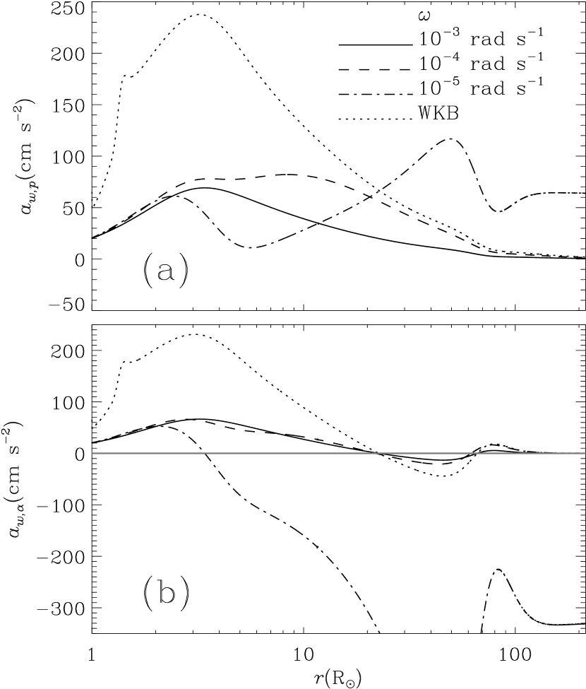
Figure 5.— Time-average of the wave acceleration exerted on (a) protons $a_{w,p}$ and (b) alpha particles $a_{w,\alpha}$ as evaluated from equation (11). Numerical results for three angular frequencies as well as for the WKB estimates are given in different line styles as indicated in panel (a). In panel (b), the wave acceleration changes sign when the profile crosses the horizontal line.

From the perspective of solar wind modeling, one may be more curious about the feedback from the waves to the background flow. To this end, Figure 5 presents the radial distribution of the acceleration exerted on (a) the protons $a_{w,p}$ and (b) alpha particles $a_{w,\alpha}$. One can see that for $\omega=10^{-3}$ and $10^{-4}$ $\rm rad~{}s^{-1}$, the wave acceleration is less effective than that in the WKB limit throughout the computational domain. However, in the low frequency case $\omega=10^{-5}$ $\rm rad~{}s^{-1}$, $a_{w,p}$ exceeds the WKB expectation considerably beyond 22.8 $R_{\odot}$. Nevertheless, in all cases the wave force tends to accelerate the protons, i.e., $a_{w,p}>0$ everywhere between the coronal base and 1 AU. However this is not the case when the alpha particles are concerned. It can be seen from Fig.5b that the wave acceleration $a_{w,\alpha}$ is negative in the interval between 22.7 and 66.1 $R_{\odot}$ in the WKB limit as well in the case $\omega=10^{-3}$ $\rm rad~{}s^{-1}$. This coincidence of the positions where $a_{w,\alpha}$ changes sign stems from the fact that beyond $\sim 10$ $R_{\odot}$, the wave is WKB-like. On the other hand, the $a_{w,\alpha}$ profile for $\omega=10^{-4}$ $\rm rad~{}s^{-1}$ changes sign at 21.8 and 61.8 $R_{\odot}$. These locations are slightly different from their counterparts in the WKB limit. When it comes to $\omega=10^{-5}$ $\rm rad~{}s^{-1}$, the $a_{w,\alpha}$ profile does not show any resemblance to the WKB expectation. In particular, the waves start to decelerate the alpha particles even in the inner corona: $a_{w,\alpha}$ is negative everywhere beyond $3.4$ $R_{\odot}$. An interesting aspect of the wave-induced acceleration is that asymptotically both $a_{w,p}$ and $a_{w,\alpha}$ approach constant values. This is understandable since in the zero-frequency limit, in the region where $R\gg R_{A}$, both $u_{p}$ and $u_{k}$ show little radial dependence. It then follows from the expressions (45) and (46) that for ion species $k$ ($k=p,\alpha$), $a_{w,k}\sim u_{k}^{2}(\ln R)^{\prime}-U_{k}u_{k}\left(\ln R\right)^{\prime}b/B_{l}\propto R^{\prime}u_{k}$. Since in the region considered, the line of force is nearly perfectly radial, one can see that $R^{\prime}$ is a constant. As a result, $a_{w,k}$ should approach a constant asymptotically.

Figure 6.— Possible modification of ion flow speeds due to the wave acceleration. Although the speeds $U_{p,corr}$ and $U_{\alpha,corr}$, evaluated from equation (47), are not computed self-consistently, their deviation from the background flow parameters represents the significance of the wave acceleration in the force balance for the two ion species. Numerical results for three angular frequencies as well as for the WKB estimates are given in different line styles as indicated.

The extent to which the wave forces may alter the ion flows can be obtained only through a self-consistent modeling by using, e.g., the iterative approach adopted by MacGregor & Charbonneau (1994): The wave equation (4.1) and the solar wind equations (8) to (10) incorporating the wave contribution are solved alternately until a convergence is met. As a first step, however, we may simply evaluate the ion speeds $U_{k,corr}$ ($k=p,\alpha$) corrected for the wave force, i.e.,

$$U_{k,corr}^{2}-U_{k}^{2}=2\int_{R_{\odot}}^{r}a_{w,k}\mathrm{d}l.$$ (47)

Figure 6 presents the radial distribution of both $U_{p,corr}$ and $U_{\alpha,corr}$ for all the frequencies considered. The background flow speed profiles are also plotted for comparison. One may see that, with the present choice of the wave amplitude, the waves have negligible effects on the ion acceleration below the Alfvén point. Beyond the Alfvén point, the effects introduced by the waves on the speed profiles become more important, especially in the low frequency case. As a matter of fact, for $\omega=10^{-5}$ $\rm rad~{}s^{-1}$ the corrected proton speed $U_{p,corr}$ reaches 785 $\rm km~{}s^{-1}$ at 1 AU where the background value is 648 $\rm km~{}s^{-1}$. As for the alpha speed, $U_{\alpha,corr}$ becomes negative beyond 100 $R_{\odot}$ due to the significant deceleration exerted on the alphas by the waves. Of course, such a situation will not appear in reality. What will happen is that the protons are accelerated whereas alphas are decelerated by the low frequency waves until the ions move at nearly identical speeds. The net effect of low-frequency waves is thus to limit the speed difference between the protons and alpha particles at large distances. However, it should be pointed out that in these regions the net work done by the low-frequency wave on the solar wind as a whole is negligible: $\sum_{k}\rho_{k}U_{k}a_{w,k}\approx 0$ and $F_{w}$ is nearly divergence free as discussed in reference to Fig.4.

6. SUMMARY AND CONCLUDING REMARKS

This study has been motivated by the apparent lack of a non-WKB analysis of Alfvén waves in a multi-fluid solar wind with differentially flowing ions. To be more specific, this study is concerned with the propagation of dissipationless, hydromagnetic (angular frequency $\omega$ well below ion gyro-frequencies), purely toroidal Alfvén waves that propagate in a background 3-fluid solar wind comprised of electrons, protons and alpha particles. Azimuthal symmetry is assumed throughout. No assumption has been made that the wavelength is small compared with the spatial scales at which the background flow parameters vary. The wave behavior at a given $\omega$ is governed by equation (4.1), which is derived from the general transport equations in the five-moment approximation. The Alfvénic point, where the combined Alfvén Mach number $M_{T}=1$ (cf. Eq.(34)), is a singular point of equation (4.1) and a regularity condition has to be imposed. For the other boundary condition, we impose a velocity amplitude of 10 $\rm km~{}s^{-1}$ at the coronal base (1 $R_{\odot}$). For the given background model of a realistic low-latitude fast solar wind, equation (4.1) is integrated numerically for three representative angular frequencies $\omega=10^{-3}$, $10^{-4}$ and $10^{-5}$ $\rm rad~{}s^{-1}$ to yield the radial distribution of the wave energy and energy flux densities as well as the wave-induced acceleration exerted on ion species.

The first conclusion concerns the applicability of the WKB approximation. Between 1 $R_{\odot}$ and 1 AU, the numerical solutions show substantial deviation from the WKB expectations. Even for the relatively high frequency $\omega=10^{-3}$ $\rm rad~{}s^{-1}$, a WKB-like behavior can be seen only in regions where $r\gtrsim 10$ $R_{\odot}$. In the low-frequency case $\omega=10^{-5}$ $\rm rad~{}s^{-1}$, the computed profiles of wave-related parameters show a spatial dependence that is distinct from the WKB one, the deviation being particularly pronounced in interplanetary space. In the inner corona $r\lesssim 4$ $R_{\odot}$, the computed ion velocity fluctuations are considerably smaller than the WKB expectations in all cases, as is the computed wave-induced acceleration exerted on protons or alpha particles. As for the wave energy and energy flux densities, they can be enhanced or depleted compared with the WKB results, depending on $\omega$.

The second conclusion is concerned with how the wave acceleration may alter the background flow parameters. In reference to Fig.6, it is found that with the current choice of base wave amplitude, the wave acceleration has little effect on the force balance for protons or alpha particles in the corona. That is, one has to invoke processes other than the non-WKB wave acceleration to accelerate the ions out of the gravitational potential well of the Sun. However, at large distances beyond the Alfvénic point, low-frequency waves may play an important role in the ion dynamics, with the net effect being to equalize the speeds of the two ion species considered.

Strictly speaking, the separation of the flow into fluctuations and a time-independent background implies that the waves are linear. However, one may have noticed that the wave amplitude $\left<b^{2}\right>^{1/2}$ at 1 AU for $\omega=10^{-5}$ s^-1 $\rm rad~{}s^{-1}$ is substantially larger than the background poloidal magnetic field strength (cf. Fig.3a). That the transverse magnetic field dominates the poloidal one demands a careful examination of the nonlinear effects other than the wave-induced acceleration. In particular, one needs to look at the generation of secondary waves and structures by the primary Alfvén waves through the source terms in the momentum equation. As discussed by Lou (1993), in the case of ideal MHD these source terms decrease sufficiently fast with radial distance asymptotically. Consequently, the first-order wave amplitudes are valid provided that the amplitude imposed at the coronal base is sufficiently small. The basic picture is expected to be the same even if a second ion species is included, although a similar discussion in the 3-fluid framework will be complicated by the richness of wave modes due to the differential proton-alpha streaming (e.g., McKenzie et al., 1993).

As has been mentioned in the introduction, Alfvén waves are dissipated in some way, and this dissipation of the primary waves should be described self-consistently. A possibility to do this is to perform a full Elsässer analysis extended to the multi-fluid case, and to express the dissipation in terms of the amplitudes of counter-propagating waves. We note that this already complicated issue will become even trickier considering the necessity to apportion the dissipated wave energy among different species.

In closing, we note that the low-frequency waves may also be important for outflows from stars other than the Sun. For instance, in the radiatively driven stellar winds, these waves will provide a further channel of momentum exchange between passive ions and line-absorbing ions in addition to the Coulomb friction. This possibility was first pointed out by Pizzo et al. (1983) in connection with the effects of stellar rotation. Due to the clear resemblance between the low-frequency Alfvén waves and stellar rotation (cf. section 3.2), their discussion also applies to the case where the star persistently emits Alfvén waves with frequencies lower than the critical one defined by equation (44). Consequently, the mass loss rate may be significantly altered. A quantitative study of this effect is beyond the scope of the present paper though.

References

- Alazraki & Couturier (1971) Alazraki, G., & Couturier, P. 1971, A&A, 13, 380
- Armstrong & Woo (1981) Armstrong, J. W., & Woo, R. 1981, A&A, 103, 415
- Banaszkiewicz et al. (1998) Banaszkiewicz, M., Axford, W. I., & McKenzie, J. F. 1998, A&A, 337, 940
- Banerjee et al. (1998) Banerjee, D., Teriaca, L., Doyle, J. G., & Wilhelm, K. 1998, A&A, 339, 208
- Bavassano et al. (2000a) Bavassano, B., Pietropaolo, E., & Bruno, R. 2000a, J. Geophys. Res., 105, 12697
- Bavassano et al. (2000b) Bavassano, B., Pietropaolo, E., & Bruno, R. 2000b, J. Geophys. Res., 105, 15959
- Belcher & Davis (1971) Belcher, J. W., & L. Davis, Jr. 1971, J. Geophys. Res., 76, 3534
- Cranmer & van Ballegooijen (2005) Cranmer, S. R., & van Ballegooijen, A. A. 2005, ApJS, 156, 265
- Dmitruk et al. (2001) Dmitruk, P., Milano, L. J., & Matthaeus, W. H. 2001, ApJ, 548, 482
- Esser et al. (1999) Esser, R., Fineschi, S., Dobrzycka, D., et al. 1999, ApJ, 510, L63
- Goldstein et al. (1995) Goldstein, M. L., Roberts, D. A., & Matthaeus, W. H. 1995, ARA&A, 33, 283
- Heinemann & Olbert (1980) Heinemann, M. & Olbert, S. 1980, J. Geophys. Res., 85, 1311
- Hollweg (1974) Hollweg, J. V. 1974, J. Geophys. Res., 79, 1357
- Hollweg et al. (1982) Hollweg, J. V., Bird, M. K., Volland, H., et al. 1982, J. Geophys. Res., 87, 1
- Hollweg & Isenberg (2002) Hollweg, J. V., & Isenberg, P. A. 2002, J. Geophys. Res., 107(A7), doi:10.1029/2001JA000270
- Isenberg & Hollweg (1982) Isenberg, P. A., & Hollweg, J. V. 1982, J. Geophys. Res., 87, 5023
- Li et al. (1999) Li, X., Habbal, S. R., Hollweg, J. V., & Esser, R. 1999, J. Geophys. Res., 104, 2521
- Li & Li (2006) Li, B., & Li, X. 2006, A&A, 456, 359
- Lou (1993) Lou, Y.-Q. 1993, J. Geophys. Res., 98, 3563
- MacGregor & Charbonneau (1994) MacGregor, K. B., & Charbonneau, P. 1994, ApJ, 430, 387
- McComas et al. (2000) McComas, D. J., Barraclough, B. L., Funsten, H. O., et al. 2000, J. Geophys. Res., 105, 10419
- McKenzie et al. (1979) McKenzie, J. F., Ip, W.-H., & Axford, W. I. 1979, Ap&SS, 64, 183
- McKenzie et al. (1993) McKenzie, J. F., Marsch, E., Baumgärtel, K., & Sauer, K. 1993, Ann. Geophysicae, 11, 341
- McKenzie (1994) McKenzie, J. F. 1994, J. Geophys. Res., 99, 4193
- Marsch et al. (1982) Marsch, E., Mühlhäuser, K.-H., Rosenbauer, K., Schwenn, R., & Neubauer, F. M. 1982, J. Geophys. Res., 87, 35
- Parker (1965) Parker, E. N. 1965, Space Sci. Rev., 4, 666
- Pizzo et al. (1983) Pizzo, V., Schwenn, R., Marsch, E. et al. 1983, ApJ, 271, 335
- Scott et al. (1983) Scott, S. L., Coles, W. A., & Bourgois, G. 1983, A&A, 123, 207
- Smith & Balogh (1995) Smith, E. J., & Balogh, A. 1995, Geophys. Res. Lett., 22, 3317
- Tu & Marsch (1995) Tu, C.-Y., & Marsch, E. 1995, Space Sci. Rev., 73, 1
- Verdini et al. (2005) Verdini, A., Velli, M., & Oughton, S. 2005, A&A, 444, 233