$\gamma^{2}$ Velorum: Orbital Solution and Fundamental Parameter Determination with SUSI

Abstract

The first complete orbital solution for the double-lined spectroscopic binary system $\gamma^{2}$ Velorum, obtained from measurements with the Sydney University Stellar Interferometer (SUSI), is presented. This system contains the closest example of a Wolf-Rayet star and the promise of full characterisation of the basic properties of this exotic high-mass system has subjected it to intense study as an archetype for its class. In combination with the latest radial-velocity results, our orbital solution produces a distance of $336^{+8}_{-7}$ pc, significantly more distant than the Hipparcos estimation (Schaerer et al. 1997; van der Hucht et al. 1997). The ability to fully specify the orbital parameters has enabled us to significantly reduce uncertainties and our result is consistent with the VLTI observational point (Millour et al., 2006), but not with their derived distance. Our new distance, which is an order of magnitude more precise than prior work, demands critical reassessment of all distance-dependent fundamental parameters of this important system. In particular, membership of the Vela OB2 association has been reestablished, and the age and distance are also in good accord with the population of young stars reported by Pozzo et al. (2000). We determine the O-star primary component parameters to be M_V(O) = $-5.63\pm 0.10$ mag, R(O) = $17\pm 2$ R_☉ and ${\cal M}$(O) = $28.5\pm 1.1$ M_☉. These values are consistent with calibrations found in the literature if a luminosity class of II–III is adopted. The parameters of the Wolf-Rayet component are M_v(WR) = $-4.33\pm 0.17$ mag and ${\cal M}$(WR) = $9.0\pm 0.6$ M_☉.

1 Introduction

The high-luminosity Wolf-Rayet (WR) stars are characterised by bright emission line spectra produced in hot, high-speed stellar winds (van der Hucht, 1992). Thought to embody the final stable stage in the evolution of very massive stars, they are candidate precursors to Type Ib/Ic supernovae (van der Hucht, 2001). The fast ($v_{\infty}\simeq 10^{3}$kms^-1) stellar winds of WR stars are responsible for prodigious mass loss ($10^{-5}$ M_☉ yr^-1), eventually stripping the star of its outer layers and forming their characteristic He-rich emission-line spectrum. Despite the ephemeral nature of this phase, these stars are important not only for understanding the evolution of massive stars but also as tracers of galactic structure and star formation (van der Hucht, 2001).

The double-lined spectroscopic binary $\gamma^{2}$ Velorum (HR 3207, HD 68273, WR 11) contains the brightest example of the WR type in the sky and has a combined visual magnitude $V\simeq 1.8$ with an O-star companion. It has a Hipparcos determined distance of $258^{+41}_{-31}$ pc (Schaerer, Schmutz & Grenon 1997; van der Hucht et al. 1997), placing $\gamma^{2}$ Vel closer to Earth than any other WR star by a factor of approximately two (Morris et al. 2000; Setia Gunawan et al. 2001). Its proximity is not the only reason that it is a key target for astronomers: the orbital motion of the two stars makes $\gamma^{2}$ Vel one of the few systems for which a direct mass determination of the components can be achieved. As such, $\gamma^{2}$ Vel provides critical tests for the theory of WR and massive star evolution. It is therefore not surprising that numerous studies of this system have been made, but in spite of its seemingly textbook status, considerable uncertainties remain.

Spectroscopic analysis of $\gamma^{2}$ Vel has been hampered by entanglement of the O-star and WR wind emission: all absorption features of the brighter O-star component are blended with emission lines from the WR wind (De Marco et al., 2000). Accounting for the WR emission is not trivial because a) multiple emission lines may contribute to the blend, b) the shape of the emission line may differ significantly from a Gaussian, c) the emission lines vary in time with some excess emission attributed to wind-wind collision phenomena, d) the extended wings of the strong O-star absorption are lost in the blend (Schmutz et al. 1997; De Marco & Schmutz 1999; Eversberg, Moffat & Marchenko 1999). This has resulted in numerous luminosity and spectral class identifications of the O-star in the literature: O7.5 (Ganesh & Bappu, 1967), O8 (Baschek & Scholz, 1971), O9 I (Conti & Smith, 1972), O8 III (Schaerer et al., 1997) and O7.5 III–V (van der Hucht, 2001).The WR component has retained its original classification of type WC8 by Smith (1968a).

The first to determine the period and some of the orbital elements by radial velocity measurements were Ganesh & Bappu (1967). Further spectroscopic studies, for example Niemela & Sahade (1980), Pike, Stickland & Willis (1983) and Moffat et al. (1986), continued to add to our knowledge of the system but discrepancies could not be resolved and observations from the IUE could ‘only be seen as muddying some already murky waters’ (Stickland & Lloyd, 1990). By correcting the O-star absorption lines due to the WR emission, Schmutz et al. (1997) believe they have the most definitive spectroscopic orbit to date. However, this type of analysis cannot determine all of the orbital elements. For example, the inclination has been estimated from the polarimetric analysis of St.-Louis et al. (1987) and further constraints were imposed by Schmutz et al. (1997), De Marco & Schmutz (1999) and De Marco et al. (2000) who used the Hipparcos distance, stellar models and spectroscopy.

Due to the high angular resolution needed, only interferometric techniques can currently be employed to accurately constrain the remaining orbital parameters. However, the southerly declination ($-47\degr 20\arcmin$) of $\gamma^{2}$ Vel places it out of reach for many interferometers of sufficient resolving power. Hanbury Brown et al. (1970) used the Narrabri Stellar Intensity Interferometer (NSII) to study this system, determining the angular semi-major axis to be $4.3\pm 0.5$ mas. Unfortunately, the signal-to-noise of their observations necessitated the adoption of the parameters of Ganesh & Bappu (1967) which have now been superseded by those of Schmutz et al. (1997). Furthermore, due to the lack of observations, the inclination could not be adequately constrained and a value $i=70\degr$ was assumed from theoretical arguments. The Very Large Telescope Interferometer (VLTI) has observed $\gamma^{2}$ Vel and produced a single angular separation and position angle (Millour et al., 2006) but has yet to improve the orbital parameters.

Reliance on distance estimations and stellar models has paved the way for further analysis of fundamental parameters, although this path has been fraught with controversy. The pre-Hipparcos distance of $\gamma^{2}$ Vel was inferred from the assumed membership of the Vela OB2 association or from statistical absolute magnitudes of similar or nearby stars. Baschek & Scholz (1971) assumed equidistance with the visual companion $\gamma^{1}$ Vel while Conti & Smith (1972) adopted 460 pc from estimates of nearby stars. The interferometric study of Hanbury Brown et al. (1970) combined with the spectroscopy of Ganesh & Bappu (1967) produced the first dynamical parallax of this system yielding $350\pm 50$ pc, although this distance is affected by the assumed values of some orbital parameters. In the 1980s, the distance to $\gamma^{2}$ Vel was assumed to be equal to that of the Vela OB2 association (450pc) with sufficient certainty as to be used in the determination of galactic WR intrinsic parameters (van der Hucht et al., 1988). The publication of the significantly different Hipparcos parallax distance of $258^{+41}_{-31}$ pc by Schaerer et al. (1997) and van der Hucht et al. (1997) caused a critical reassessment of all $\gamma^{2}$ Vel parameters that are distance dependent – the absolute magnitude of the components, the spectral class of the O-star primary, the mass-loss of the WR star etc. The Hipparcos distance has been challenged by the discovery of a low-mass, pre-main-sequence stellar association in the direction of $\gamma^{2}$ Vel and the Vela OB2 association. Pozzo et al. (2000) argue these low-mass stars are associated with $\gamma^{2}$ Vel and approximately coeval at a distance consistent with earlier estimates of 360–490 pc. The single measurement by the VLTI has yielded a measure of the distance to $\gamma^{2}$ Vel of $368^{+38}_{-13}$ pc (Malbet et al. 2006; Millour et al. 2006) placing the system farther from the Hipparcos distance and closer to the Vela OB2 association.

In Section 3 we provide the first complete orbital solution for $\gamma^{2}$ Vel determined by long-baseline optical interferometry. In combination with the latest radial velocity measurements, the tightly constrained distance, spatial scale and mass of the components are quantified and compared to previous estimates in Section 4. The details of our observations and a description of the parameter fitting procedure are described in Section 2 and Section 3 respectively.

2 Observations and Data Reduction

Table 1: Adopted parameters of reference stars used during observations.

HR	Name	Spectral	V	UD Diameter	Separation
		Type		(mas)	from $\gamma^{2}$ Vel
3090	J Pup	B0.5 Ib	4.24	$0.18\pm 0.03^{a}$	2.96°
3117	$\chi$ Car	B3I Vp	3.47	$0.36\pm 0.06^{a}$	6.02°
3165	$\zeta$ Pup	O5f	2.25	$0.41\pm 0.03^{b}$	7.41°
3468	$\alpha$ Pyx	B1.5 III	3.68	$0.27\pm 0.06^{a}$	15.54°

Notes:	a Based on NSII measurements of similar type stars.
	b Hanbury Brown, Davis & Allen (1974).

Measurements of the squared visibility (i.e. the squared modulus of the normalised complex visibility) or $V^{2}$ were completed on a total of 24 nights using the Sydney University Stellar Interferometer (SUSI, Davis et al. 1999). Interference fringes were recorded with the red beam-combining system using a filter with centre wavelength and full-width half-maximum of 700 nm and 80 nm respectively. This system was outlined in Tuthill et al. (2004) and is to be described in greater detail in Davis et al. (in preparation).

Interference fringes produced by a pupil-plane beam-combiner were modulated by repeatedly scanning the optical delay about the white light fringe position. The two outputs of the beam-combiner were detected by avalanche photo-diodes. An observation unit consisted of a set of 1000 scans traversing 140 $\mu$m in optical delay digitised into 1024 steps of 0.2 ms samples.

During post-processing of the data, the two signals were differenced to mitigate noise introduced by scintillation and the squared visibility was estimated after bias subtraction for each observation. A nonlinear function was applied to partially correct for residual seeing effects (Ireland, 2006).

Reference stars close $\gamma^{2}$ Vel on the sky, chosen to provide calibration of the system response, were interleaved with the target observations. The system response as a function of time was quantified using the adopted stellar parameters of the calibrator stars given in Table 1. Measurements of $V^{2}$ were finally produced by linearly interpolating the system response to the time of target observation and scaling the observed squared visibility appropriately. This procedure resulted in a total of 278 estimations of $V^{2}$ as summarised in Table 2. The majority of the observations were completed in excellent conditions and the atmospheric correction to the final $V^{2}$ values was small with a mean value of the order 2 percent.

Table 2: Summary of observational data. The night of the observation is given in cols 1 and 2 as a calendar date and a mean MJD. Col 3 is the mean orbital phase calculated from the values in Table 3. The baseline and the mean projected baseline (in units of metres) are given in Col 4-5 respectively. Reference stars and the the number of squared visibility measures for a night are listed in the last two columns.

Date	MJD	Phase	Nominal	Projected	Reference	# V2
			Baseline	Baseline	Stars
2005 Mar 10	53439.52	0.26	80	75.52	$\zeta$ Pup, $\chi$ Car, J Pup, $\alpha$ Pyx	10
2005 Mar 11	53440.48	0.28	80	75.93	$\zeta$ Pup, $\chi$ Car, $\alpha$ Pyx	15
2005 Mar 12	53441.48	0.29	80	75.78	$\zeta$ Pup, $\chi$ Car, $\alpha$ Pyx	12
2005 Dec 17	53721.70	0.86	80	76.19	$\zeta$ Pup, $\chi$ Car, $\alpha$ Pyx	9
2005 Dec 18	53722.69	0.87	80	76.18	$\zeta$ Pup, $\chi$ Car, J Pup	13
2005 Dec 19	53723.68	0.88	80	76.24	$\zeta$ Pup, $\chi$ Car, J Pup	12
2005 Dec 20	53724.68	0.89	80	76.19	$\zeta$ Pup, $\chi$ Car, J Pup	12
2005 Dec 23	53727.62	0.93	80	76.02	$\zeta$ Pup, $\chi$ Car	6
2005 Dec 29	53733.67	0.01	80	76.02	$\zeta$ Pup, $\chi$ Car	14
2005 Dec 30	53734.65	0.02	80	76.04	$\zeta$ Pup, $\chi$ Car	10
2005 Dec 31	53735.66	0.03	80	75.97	$\zeta$ Pup, $\chi$ Car	16
2006 Jan 01	53736.62	0.05	80	76.22	$\zeta$ Pup, $\chi$ Car	9
2006 Jan 02	53737.62	0.06	80	76.04	$\zeta$ Pup, $\chi$ Car, J Pup	15
2006 Jan 07	53742.64	0.12	80	76.30	$\zeta$ Pup, $\chi$ Car	9
2006 Jan 08	53743.62	0.14	80	76.28	$\zeta$ Pup, $\chi$ Car	9
2006 Jan 09	53744.65	0.15	80	76.08	$\zeta$ Pup, $\chi$ Car, J Pup	13
2006 Feb 08	53774.61	0.53	80	75.39	$\zeta$ Pup, $\chi$ Car	10
2006 Feb 10	53776.60	0.56	80	75.35	$\zeta$ Pup, $\chi$ Car	15
2006 Feb 11	53777.57	0.57	80	75.11	$\zeta$ Pup, $\chi$ Car	24
2006 Feb 13	53779.56	0.59	80	75.13	$\zeta$ Pup, $\chi$ Car	21
2006 May 11	53866.37	0.70	5	4.71	$\zeta$ Pup, $\chi$ Car	5
2006 May 11	53866.42	0.70	30	27.47	$\zeta$ Pup, $\chi$ Car	4
2006 Jun 17	53903.38	0.17	5	4.30	$\zeta$ Pup, $\chi$ Car	7
2006 Jun 18	53904.37	0.18	15	12.95	$\zeta$ Pup, $\chi$ Car	6

3 Orbital Solution

The theoretical response of a two aperture interferometer to the combined light of a binary star can be given by (Hanbury Brown et al., 1970)

$$V^{2}=\frac{V_{1}^{2}+\beta^{2}V_{2}^{2}+2\beta|V_{1}||V_{2}|\cos(2\pi\mn@boldsymbol{b}\cdot\mn@boldsymbol{\rho}/\lambda)}{(1+\beta)^{2}},$$ (1)

where $V_{1}$, $V_{2}$ are the visibilities of the primary and secondary respectively and $\beta<1$ is the brightness ratio of the two stars in the observed bandwidth. The angular separation vector of the secondary with respect to the primary is given by $\mn@boldsymbol{\rho}$ (measured East from North), $\mn@boldsymbol{b}$ is the baseline vector projected onto the plane of the sky and $\lambda$ is the centre observing wavelength. The observed $V^{2}$ will vary throughout the night due to Earth rotation of $\mn@boldsymbol{b}$ and the orbital motion of the binary. The Keplerian orbit of a binary star, i.e. $\mn@boldsymbol{\rho}$ as a function of time, can be parameterized with seven elements: the period $P$, semi-major axis $a$, eccentricity $e$, epoch of periastron $T_{0}$, the longitude of periastron $\omega$, the longitude of ascending node $\Omega$ and the inclination $i$. When using two-aperture optical interferometry, the phase of the complex visibility is lost and hence, $\omega$ and $\Omega$ have an ambiguity of 180°. This stems from the fact that the identity of the components cannot be determined. Radial velocity measurements can be used to remove the ambiguity of $\omega$ but that of $\Omega$ remains. Interferometers with three or more apertures can use closure phase techniques to identify the components and hence remove the 180°ambiguity of $\Omega$.

3.1 Component Visibilities

In the simplest case, stars can be modeled by a disc of uniform irradiance with angular diameter $\theta$. The visibility is then given by

$$V=\frac{2J_{1}(\pi|\mn@boldsymbol{b}|\theta/\lambda)}{\pi|\mn@boldsymbol{b}|\theta/\lambda},$$ (2)

where $J_{1}$ is a first order Bessel function. Real stars are limb-darkened, therefore corrections to the uniform disc diameter are needed to find an estimate of the true angular diameter. In the case of a compact atmosphere, the corrections are small but this may not be the case with extreme-limb darkened stars or stars with extended atmospheres (Tango & Davis, 2002). In the case of emission line stars, care must be taken to ensure that only the continuum is observed (i.e. free of line emission) because a layer that forms an emission line cannot be assumed to be at the same radius as the continuum. The optically thick stellar wind of WR stars not only produces emission lines but also obscures the hydrostatic core surface (Moffat & Marchenko, 1996).

Over SUSI’s wide observing band, emission lines contributed a significant portion of the detected light. The expected spectral response of SUSI (the combination of the 700 nm filter profile and fig. 5 of De Marco et al. 2000) was used to estimate that four emission lines contribute approximately 32 percent of the light received from the WR component during our observations. Three lines are blends of HeI–CIII, CIII–HeI and CII–CIII at $\lambda\lambda$674.1, 706.6, 723.0 nm respectively. The remaining line is due to HeII at $\lambda$656.0 nm.

As each emission line corresponds to a different excitation/ionisation, it follows that each line could be formed at a different radius in the stellar wind. Moreover, emission lines may form over a range of radii. Hillier (1989) and Dessart et al. (2000) have used WR models to predict the line formation stratification in the stellar wind. Niedzielski (1994) and Schulte-Ladbeck, Eenens & Davis (1995) have shown that observed WR emission lines have differing equivalent widths and concluded that these differences were evidence of excitation/ionisation stratification within the WR stellar wind. In the case of $\gamma^{2}$ Vel, Hanbury Brown et al. (1970) estimated the uniform disc angular diameter of the $\lambda 465.0$ nm CIII emission region to be $2.05\pm 0.19$ mas and the analysis of the VLTI included modeling of the relevant WR IR emission line layers as uniform discs, each with a small difference in diameter (Millour et al., 2006).

Unfortunately, the radii of the detected emission line forming layers have not been measured over SUSI’s optical range and SUSI’s red system presently has no way of isolating a single emission line. One possibility is that the four detected emission line forming layers are at essentially equal radii allowing a simple single uniform disc model of the emission. However, a Gaussian irradiance profile may be more applicable if the layers are spread in radii.

We therefore analyse the interferometric data using two models of the WR star, each with a continuum core as a disc of uniform irradiance with angular diameter $\theta_{\rm C}$. The emission line layers are modeled to be either a single uniform disc of angular diameter $\theta_{\rm U}$ or a Gaussian shell with angular full-width half-maximum of $\theta_{\rm G}$ contributing $I_{\rm E}$ of the detected irradiance. The theoretical visibilities for these models are:

$$V_{\rm WR,U}=(1-I_{\rm E})\frac{2J_{1}(\pi|\mn@boldsymbol{b}|\theta_{\rm C}/\lambda)}{\pi|\mn@boldsymbol{b}|\theta_{\rm C}/\lambda}+I_{\rm E}\frac{2J_{1}(\pi|\mn@boldsymbol{b}|\theta_{\rm U}/\lambda)}{\pi|\mn@boldsymbol{b}|\theta_{\rm U}/\lambda}$$ (3)

$$V_{\rm WR,G}=(1-I_{\rm E})\frac{2J_{1}(\pi|\mn@boldsymbol{b}|\theta_{\rm C}/\lambda)}{\pi|\mn@boldsymbol{b}|\theta_{\rm C}/\lambda}+I_{\rm E}\exp\left[\frac{-\pi^{2}}{4\ln 2}\frac{\theta_{\rm G}^{2}|\mn@boldsymbol{b}|^{2}}{\lambda^{2}}\right]$$ (4)

The O-star primary is modeled as a uniform disc of angular diameter $\theta_{\rm O}$ as per equation (2). Note that the brightness ratio $\beta$ in equation (1) is usually given in reference to the continuum irradiance detected in the observing band i.e. free from emission lines. As our observing band is contaminated with emission lines it is convenient to introduce the relative brightness $\beta^{\prime}$ of the WR component (including emission lines) to that of the O-star in the observing band. The simple relation

$$\beta=(1-I_{\rm E})\beta^{\prime}$$ (5)

can then be used to estimate the usual continuum brightness ratio.

3.2 Fitting Procedure and Uncertainty Estimation

Equation (1) is strictly only valid for observations over very narrow bandwidths. For real detection systems wide bandwidth effects can reduce the observed $V^{2}$. Tango & Davis (2002) present corrections which can be applied to wide bandwidth interferometric observations of single stars. In the case of binary stars, the way in which the wide bandwidth affects the observed squared visibility ($V^{2}$) is dependent on the detection system and subsequent calculations (Boden, 1999). For a scanning detection system (such as the one used at SUSI) the modulating term in equation (1) will be reduced by a factor that is dependent on the separation of the component phase centres in delay space and the spectral response of the interferometer. Approximating the spectral response as a Gaussian of centre wavelength $\lambda_{0}$ with full-width half-maximum $\Delta\lambda$ and for convenience defining $\psi=2\pi\mn@boldsymbol{b}\cdot\mn@boldsymbol{\rho}/\lambda_{0}$, then the equivalent to equation (1) giving $V^{2}$ for a binary star for the case of a wide spectral bandwidth is:

$$V^{2}=\frac{V_{1}^{2}+\beta^{2}V_{2}^{2}+2\beta r(\psi)|V_{1}||V_{2}|\cos(\psi)}{(1+\beta)^{2}},$$ (6)

where

$$r(\psi)=\exp\left[\frac{-\Delta\lambda^{2}}{\lambda_{0}^{2}}\frac{\psi^{2}}{32\ln 2}\right].$$ (7)

The term $r(\psi)$ corresponds to the autocorrelation of the Gaussian envelope of the interference pattern. As $\Delta\lambda$ approaches zero, i.e. a narrow bandwidth, then equation (6) reduces to equation (1).

In the case of $\gamma^{2}$ Vel, the emission lines (in an otherwise near-Gaussian spectral response determined by the 700 nm filter profile and fig. 5 of De Marco et al. 2000) alter the shape of the modulated interference fringes, further complicating the estimation of $V^{2}$. Detailed numerical simulations showed that the error introduced when approximating the spectral response as Gaussian was smaller than the associated measurement error. Hence a Gaussian approximation of the spectral response was deemed adequate.

Initial values of $i$ and $\Omega$ were found via a coarse search of parameter space with the remaining orbital parameters limited to within 3 standard deviations of the values given in Schmutz et al. (1997) and the stellar model parameters ($\theta_{\rm O}$, $\theta_{\rm C}$, $\theta_{\rm G}$/$\theta_{\rm U}$, $\beta$, $I_{\rm E}$) were estimated using Hanbury Brown et al. (1970), Schmutz et al. (1997) and De Marco et al. (2000).

The final estimation of parameters was completed using $\chi^{2}$ minimization as implemented by the Levenberg-Marquardt method to fit equation (6) to the observed $V^{2}$. As the radial velocity measures have occurred over a long time frame of many periods, the spectroscopically determined period will be of higher accuracy than that determined by interferometry. Therefore the period given in Schmutz et al. (1997) was adopted and the remaining orbital parameters were allowed to vary. The angular diameters were initially fixed to 0.44 mas for the primary (from Hanbury Brown et al. 1970) and 0.22 mas for the WR continuum core i.e. a continuum radius of 6 R_☉ at the Hipparcos distance of 258 pc. The emission line contribution for each model was fixed to 32 percent of the received WR star irradiance and the brightness ratio $\beta^{\prime}$ was a free parameter. These values are not critical as the resolution of the SUSI configuration during observations is such that the WR continuum is essentially unresolved. Moreover $V_{1}$, $V_{2}$ & $\beta^{\prime}$ (and hence $\theta_{\rm O}$, $\theta_{\rm C}$, $\theta_{\rm G}$/$\theta_{\rm U}$ & $I_{\rm E}$) are coupled and only affect the estimated orbital solution from equation (6) if highly inappropriate values are adopted.

When finding the minimum of the $\chi^{2}$ manifold, the non-linear fitting program calculates the inverse of the covariance matrix. The diagonal elements are used to derive the formal uncertainties of the fitted parameters. As equation (6) is non-linear and the visibility measurement errors may not strictly conform to a normal distribution, the formal uncertainties may be underestimates. To confirm the accuracy of the values derived from the covariance matrix, three uncertainty estimation methods were adopted.

Firstly, the model visibilities of each observation were subjected to Monte Carlo realisation of the measurement error distribution to produce synthetic data sets. Secondly, the bootstrap method (Press et al., 1992) was employed to produce a second population of synthetic data. By randomly sampling with replacement, a synthetic data set is formed. The bootstrap method has the advantage that the measurement error distribution is not assumed to be known as per Monte Carlo but may not produce a representative sample. The synthetic data sets from each method were used to estimate the model parameters with the same non-linear fitting program, thus building a distribution of each model parameter.

The final uncertainty estimation method involves a likelihood based random walk through parameter space using a Markov chain Monte Carlo (MCMC) simulation implemented with a Metropolis-Hastings algorithm (see Chapter 12 of Gregory 2005a for an introduction to MCMC). This approach yields the full marginal posterior probability density function (PDF) but may fail to fully explore pathologically narrow probability peaks in a reasonable number of iterations (Gregory, 2005b). Furthermore, the current knowledge of the system can be included in the analysis by assuming an a priori distribution. For example, the effect of adopting the spectroscopic period (and associated uncertainty) on the remaining orbital parameters can be included into the uncertainty estimation of the remaining model parameters.

3.3 Results

Table 3: Comparison of the fitted parameters of this work with those found in the literature.

Parameter	Unit	This Work	Literature	Ref
$P$	days	$(78.53\pm 0.01)^{a}$	$78.53\pm 0.01$	S97
$a\arcsec$	mas	$3.57\pm 0.05$	$4.3\pm 0.5$	HB70
$e$		$0.334\pm 0.003$	$0.326\pm 0.01$	S97
$T_{0}$	MJD	$50120.4\pm 0.4$	$50120\pm 2$	S97
$\omega$	deg	$67.4\pm 0.5$	$68\pm 2$	S97
$\Omega$	deg	$247.7\pm 0.4$	$[-80,-20]^{bc}$	SL87
			$142^{b}$	S97
$i$	deg	$65.5\pm 0.4$	$65\pm 8$	S97
			$63\pm 3$	DM00
$\theta_{\rm O}$	mas	$0.47\pm 0.05$	$0.44\pm 0.05$	HB70
$\theta_{\rm C}$	mas	$(0.17\pm 0.08)^{a}$	-	-
$\theta_{\rm G}$	mas	$1.3\pm 0.3$	-	-
$\theta_{\rm U}$	mas	$1.7\pm 0.2$	-	-
$\beta^{\prime}$		$0.45\pm 0.02$	-	-
$I_{\rm E}$		$(0.32\pm 0.03)^{a}$	$0.32$	DM00

^a adopted parameters, ^b definition is ambiguous, see text for more details, ^c square brackets denote a range.
HB70: Hanbury Brown et al. (1970); SL87: St.-Louis et al. (1987); S97: Schmutz et al. (1997); DM00: De Marco et al. (2000)

Initial analysis resulted in orbital parameters that, when combined with the spectroscopic values as shown in Section 4.2, produced a distance of approximately 330 pc. Consequently, the angular diameter of the WR continuum core was revised to 0.17 mas (consistent with radius expectations at this new distance) which had a negligible small effect the fitted orbital parameters. We note that the WR core is essentially unresolved and therefore any diameter uncertainty (such as limb-darkening corrections to the equivalent uniform disc angular diameter) are insignificant.

The results of the two models (uniform disc and Gaussian shell) were completely consistent in all orbital parameters and the final values of the fitted parameters are given in Table 3. Example data from two nights with the fitted models is shown in Fig. 1 and the projected orbit on the plane of the sky is shown in Fig. 2. The reduced $\chi^{2}$ of the two fits were approximately 2.2 implying that the formal measurement errors calculated by the data reduction software are underestimated by 49 percent. Therefore the measurement uncertainties were scaled by 1.49 before the parameter uncertainties were estimated using the techniques outlined in Section 3.2. The Monte Carlo and bootstrap methods were set to each generate $10^{3}$ synthetic data sets while the MCMC simulations completed $10^{7}$ iterations. All combinations of model and uncertainty estimation methods produced similar distributions of the free parameters which were, for the orbital elements, Gaussian in appearance. Furthermore, the standard deviation of each model parameter from all uncertainty methods were consistent to within rounding. The standard deviations derived from the MCMC simulations were only slightly larger as the probability space of all parameters was explored: the period, WR continuum core diameter and emission line contribution varied within a Gaussian likelihood with assumed values given in Table 3. The distributions of the emission region parameters were somewhat asymmetric with a larger tail at higher values. This is a direct result of the small number of short baseline measurements combined with the coupling of the component visibilities and the brightness ratios. All uncertainties quoted in Table 3 are the standard deviation values of the MCMC simulations as we believe they represent the most realistic and conservative parameter uncertainty estimates for our data set.

Figure 1: Data from the nights of 2005 Mar 11 and 2006 Feb 13 where each data point represents a measure of $V^{2}$ with the associated formal error. The values of Table 3 have been been used to show the uniform disc (solid) and Gaussian shell (dashed) emission layer models.

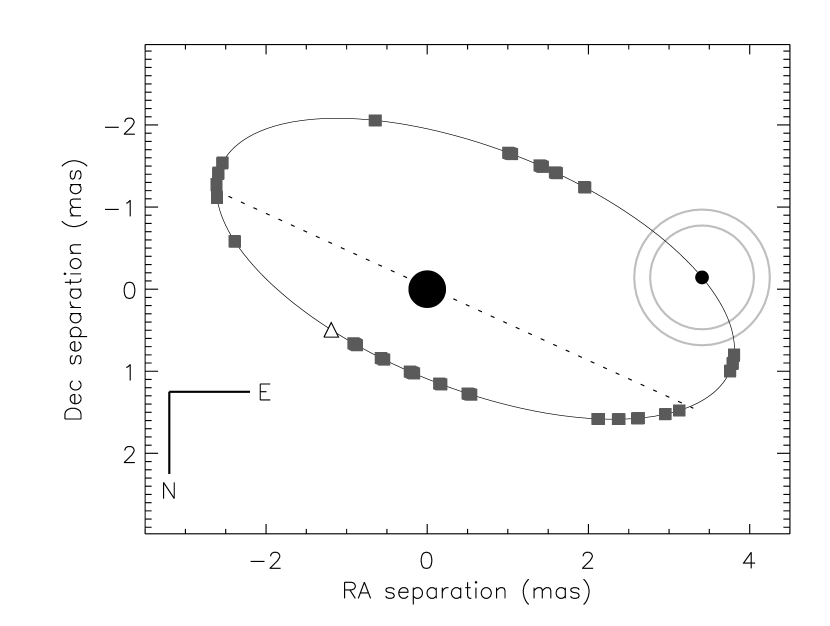
Figure 2: The relative orbit (solid line) of the WR-star about the O-star projected on the plane of the sky at an orbital phase of 0.4. The dotted line is the line-of-nodes, the open triangle signifies periastron and the grey squares are parts of the orbit that were observed with SUSI. The stellar components (filled circles) are drawn to scale using the values of Table 3. The full-width half-maximum of the Gaussian shell and the angular diameter of the uniform disc emission line layer models are shown as the grey circles about the WR component.

There is no evidence that the visual companion $\gamma^{1}$ Vel or the nearby K4 V star detected by Tokovinin et al. (1999) affect our data. $\gamma^{1}$ Vel is approximately 2.5 magnitudes fainter and separated by 41″  from $\gamma^{2}$ Vel; the K4 V star has a separation from $\gamma^{2}$ Vel of approximately 4.7″  and is approximately 14.8 magnitudes fainter (Tokovinin et al., 1999). These stars are either out of the field-of-view or too faint to be detected by SUSI.

The orbital elements derived from radial velocity measurements (Schmutz et al., 1997) are consistent with our data as is the inclination inferred by Schmutz et al. (1997) and De Marco et al. (2000). The discrepant angular semi-major axis of Hanbury Brown et al. (1970) is largely due to their adoption of the inclination ($a$ and $i$ are co-dependent as shown in Hummel et al. 1993). This correlation between $a$ and $i$ was confirmed by the ad-hoc fixing of the inclination as per Hanbury Brown et al. (1970) and the resultant angular semi-major axis was found to be consistent with their value.

The single angular separation vector of Millour et al. (2006) could be used to remove the 180°ambiguity in our value of $\Omega$. However, Millour et al. (2006) have stated their belief that they have identified the components correctly but are cautiously awaiting the final analysis of calibration data. Therefore, we tentatively set the position angle of the ascending node to that given in Table 3. Using the final orbital values at the epoch of the VLTI measurement, the separation of the components is $3.85\pm 0.06$  mas and the WR component is located $80\pm 1\degr$ (measured Eastwards from North) relative to the O-star. These values are marginally consistent with the VLTI measurement of $3.62^{+0.11}_{-0.30}$ mas and $73^{+9}_{-11}$ deg given in Millour et al. (2006).

3.4 Polarimetry Analysis

Polarimetric analyses of $\gamma^{2}$ Vel have produced the only pre-existing estimations of the position angle of the ascending node. However, the parameter, $\Omega$, quoted in the polarimetry literature is not the position angle of the ascending node but rather the position angle of the rotation axis (orbit normal) projected on to the plane of the sky (Brown, McLean & Emslie, 1978). This angle is included in the polarimetry analysis to account for the rotation of the binary system in relation to the coordinate system of the observed Stokes parameters $Q$ and $U$. In the plane of the sky, the relationship between the two definitions of $\Omega$ is a simple difference of 90°. However, the polarimetry rotation parameter $\Omega$ is usually defined in the $Q$-$U$ plane (see Robert et al. 1989) and hence an additional factor of two is introduced i.e.

$$\Omega_{\it an}=\frac{\Omega_{\it ra}}{2}\pm 90$$ (8)

where $\Omega_{\it an}$ and $\Omega_{\it ra}$ are the position angles of the ascending node in the plane of the sky and the projected rotation axis in the $Q$-$U$ plane respectively. The addition or subtraction of 90°  is dependent on the orientation of the binary orbit with respect to the North Celestial pole. Unfortunately neither St.-Louis et al. (1987) nor Schmutz et al. (1997) give details of which plane their quoted $\Omega_{\it ra}$ is measured in. For the range given in St.-Louis et al. (1987) $\Omega_{\it an}$ could be 190°–250°or 230°–260°if transformed from the plane of the sky or from the $Q$-$U$ plane respectively. Thus, the values of St.-Louis et al. (1987) are compatible with the interferometric value regardless of which plane their $\Omega$ value is measured. The $\Omega_{\it an}$ value of Schmutz et al. (1997) could be 232°(plane of the sky) or 251°($Q$-$U$ plane) respectively. Thus $\Omega_{\it an}$ derived from the $Q$-$U$ plane is close to our value. However, without an estimate of the uncertainty we cannot determine its consistency with our value.

As polarimetric data of $\gamma^{2}$ Vel are the only other available experimental values to estimate the position angle of the ascending node and the inclination (and to update the polarimetric mass-loss rate determined by St.-Louis et al. 1988 in Section 4.7) the polarimetry data of St.-Louis et al. (1987) were reanalysed using the model of Brown et al. (1982) (with the corrections made by Simmons & Boyle 1984) and the rotation angle $\Omega_{\it ra}$ included in the $Q$-$U$ plane as per Robert et al. (1989). A $\chi^{2}$ minimization was performed with the period and eccentricity fixed to the interferometric values given in Table 3. The starting values for the remaining parameters were found using the interferometric values given in Table 3. The best fit values were $T_{0}=50120.9$ MJD, $\lambda_{p}=163\degr$, $\Omega_{\it ra}=303\degr$, $i=66\degr$, $\tau_{*}=0.036$, $Q_{0}=0.077$ and $U_{0}=-0.077$. Converting to usual binary star parameters, $\lambda_{p}=\omega+90\degr$ and equation (8) give $\omega=73\degr$ and $\Omega_{\it an}=242\degr$. A $10^{7}$ iteration MCMC simulation was performed to investigate the effect that the assumed parameter and eccentricity values have on those that were fitted. All parameters with the exception of the inclination produced Gaussian PDFs centred roughly on the best fit values. However, the PDF of the inclination had multiple peaks with 90 percent of the probability contained between 64.5°and 77.5°. This confirms the statement by Schmutz et al. (1997) that the inclination cannot be accurately constrained by the available polarimetry data. The PDF of $\Omega_{\it an}$ produces an uncertainty of approximately 4°and hence our polarimetric value of $\Omega_{\it an}$ is consistent with the interferometrically determined value.

4 Discussion

4.1 Wind-Wind Interactions

The orbital values of Table 3 indicate that the angular separation at periastron is approximately 1.29 mas suggesting that the wind of the O-star primary may interact with the emission line forming layers of the WR wind. Moreover, a higher temperature and density colliding winds zone (as inferred by the X-ray spectrum of $\gamma^{2}$ Vel Willis, Schild & Stevens 1995; Stevens et al. 1996; Henley, Stevens & Pittard 2005) may also affect the appearance of the emission line forming layers. However, the angular diameter of these layers, whether modeled as a uniform disc or Gaussian irradiance distribution, is not adequately constrained by our data. The effect of an irradiance asymmetry due to wind-wind interactions on the orbital parameters is considered to be negligibly small as the WR wind is expected to dominate that of the O-star. Furthermore, the short baseline data, which should be most strongly affected, are limited and were collected during an orbital phase when the O-star was outside the estimated emission line forming layers.

4.2 Distance

The distance to a double-lined spectroscopic binary star that has a well-determined visual or interferometric orbit can be found using the dynamical parallax (Heintz, 1978):

$$\pi_{d}=\frac{a\arcsec}{(a_{1}+a_{2})}.$$ (9)

The semi-major axis of the primary (secondary) component orbit about the system centre-of-mass, $a_{1}$($a_{2}$), is measured in astronomical units.

Using the semi-amplitude of the component radial velocity given in Schmutz et al. (1997), ($K_{1}=38.4\pm 2$ kms^-1, $K_{2}=122\pm 2$ kms^-1) and the interferometric orbital values, $a_{1}$ and $a_{2}$ were calculated (in km) using

$$a_{1,2}=\frac{43200K_{1,2}P\sqrt{1-e^{2}}}{\pi\sin i}.$$ (10)

These values are given in Table 4. The resulting dynamical parallax is $\pi_{d}=2.97\pm 0.07$ mas which yields a distance of $336^{+8}_{-7}$ pc.

Compared to the Hipparcos (Schaerer et al. 1997; van der Hucht et al. 1997) and the VLTI distance (Millour et al., 2006) our uncertainty in the measured distance is lower by an about order of magnitude. Moreover, there is considerable contrast between the distance determinations. It has been shown that the dynamical parallax of some binary stars can be significantly different to the Hipparcos parallax (Davis et al. 2005; Tango et al. 2006). Binary motion can influence the Hipparcos value and where possible, has been included in the data reduction (Lindegren, 1997). The $\gamma^{2}$ Vel entry in the Hipparcos catalogue (ESA, 1997) indicates that it was not treated as binary but it is entered into the Variability Annex: Unsolved variables. Furthermore, a critical reassessment of the Hipparcos catalogue has identified a number of defects in the data (van Leeuwen, 2005) and a new reduction of the raw data is in progress (van Leeuwen & Fantino, 2005). The preliminary revision to the Hipparcos parallax of $\gamma^{2}$ Vel is $3.35\pm 0.29$ mas (van Leeuwen, private communication) i.e. a distance of $299^{+28}_{-24}$ pc which is marginally consistent with our value. The VLTI distance (Millour et al., 2006) relies on a single angular separation measure and assumed orbital elements from the literature which are inferior to our interferometric values.

The $\gamma^{2}$ Vel Hipparcos parallax raised the question of the assumed membership of the Vela OB2 association due to the disparity of their distances: 258 pc vs 450 pc. The Hipparcos proper motion and parallaxes of nearby OB associations including Vela OB2 were analysed by de Zeeuw et al. (1999) who concluded that $\gamma^{2}$ Vel was an edge member with probability of 64 percent. The 93 members produce a mean distance of $410\pm 12$ pc (de Zeeuw et al., 1999) i.e. a mean parallax of approximately 2.44 mas. Using fig. 11 of de Zeeuw et al. (1999) it was estimated that 60 percent of the Vela OB2 members lie within 0.5 mas of the mean value. Furthermore, Pozzo et al. (2000) model the Hipparcos parallax dispersion as a Gaussian of standard deviation 0.68 mas. Our parallax moves $\gamma^{2}$ Vel from the edge of Vela OB2 to well within the association. Using the Galactic coordinates of $\gamma^{2}$ Vel in van der Hucht (2001) (and a Sun-Galactic centre distance of 8 kpc) the revised Galactocentric distances are $R_{\rm GC}=7.97$ kpc and $z_{\rm GC}=-45$ pc. We estimate an uncertainty in $R_{\rm GC}$ of 0.01 kpc and $z_{\rm GC}$ of 1 pc which are a factor of four less than those estimated with the Hipparcos distance. Compared to values found in the literature ($R_{GC}=8$ kpc, $z_{GC}=-35$ pc, van der Hucht 2001) our values place $\gamma^{2}$ Vel farther from Galactic plane but at approximately the same distance from the Galactic centre.

4.3 Component Magnitudes

The absolute visual magnitude of the system and component stars can be redetermined using our distance. There is the possibility of broadband photometry (Johnson et al. 1966; Cousins 1972) suffering contamination by the WR emission lines (Smith 1968b; De Marco et al. 2000) and studies of galactic WR distributions and intrinsic parameters almost exclusively use narrowband ‘line-free’ photometry (e.g. Smith 1968b; Conti et al. 1983; Conti & Vacca 1990). The mean and standard deviation of narrowband apparent magnitude and extinction values found in the literature are $v=1.73\pm 0.03$ mag (van der Hucht et al. 1988; Smith, Shara & Moffat 1990; Conti & Vacca 1990; van der Hucht et al. 1997; De Marco et al. 2000) and $A_{v}=0.09\pm 0.06$ mag (Conti & Vacca 1990; De Marco et al. 2000; van der Hucht 2001). Therefore, combining these values with our distance we obtain the system absolute magnitude of $M_{v}({\rm WR+O})=-5.99$.

The component absolute magnitudes in both narrowband ($v$) and broadband ($V$) can then be found using the component brightness ratio in $v$ and $M_{v}-M_{V}=-0.1$ mag (van der Hucht, 2001). The output brightness ratio $\beta^{\prime}$ from the fitting procedure and the estimated emission line contribution $I_{\rm E}$ produce a continuum brightness ratio in our observing band of $\beta=0.31\pm 0.03$. This is consistent with the expected brightness ratio at 700nm of $0.35\pm 0.04$ determined from fig. 1 of De Marco et al. (2000). We therefore adopt the $v$ brightness ratio of De Marco et al. (2000) rather than scaling the continuum brightness ratio in our observing band. We obtain $M_{v}$(WR)$=-4.33\pm 0.17$ mag and $M_{V}$(O)$=-5.63\pm 0.10$ mag (from $M_{v}$(O)$=-5.73\pm 0.10$ mag) where the estimates of the magnitude uncertainties include the distance, reddening and the component brightness ratio. The uncertainties in previous estimates of the distance to $\gamma^{2}$ Vel have dominated error determinations of the component absolute magnitudes (van der Hucht et al. 1997). This limitation has now been removed with our measurement.

4.4 O-star Component

The most recent classification of the O-star spectral type is O7.5 given by De Marco & Schmutz (1999). They also deduce a bright-giant luminosity class (II) from analysis of their synthetic HeII line $\lambda 468.6$ nm as other lines are unavailable due to assumed metallicity in their model and blending effects prevent an observational determination. The recent spread-spectrum interferometric analysis of Millour et al. (2006) has found the O-star models that best fit their data have gravity values more in line with a super-giant classification. However, the Hipparcos distance produces $M_{V}$(O)$\simeq-5.1$ mag which is more consistent with a giant or dwarf hence the O7.5 III–V classification in the VIIth catalogue of galactic Wolf-Rayet stars (van der Hucht, 2001). Moreover, the calibration of physical parameters of O-stars has evolved as stellar models develop and clear separation into only three luminosity classes I, III & V has become standard. Assuming a spectral type of O7.5, our $M_{V}$(O) is consistent with a giant classification using Howarth & Prinja (1989) or Vacca, Garmany & Shull (1996) but falls between a giant and a super-giant with the calibration of Martins, Schaerer & Hillier (2005). Therefore a luminosity class of II–III for the O-star seems appropriate until the knowledge of this area of the HR diagram improves.

The radius of the O-star is obtained from the measured angular diameter and distance to the system was found to be $17\pm 2$ R_☉. This is in excellent agreement with the earlier measurement by Hanbury Brown et al. (1970). A radius of $17$ R_☉ falls between all giant and super-giant calibrations found in the literature (Howarth & Prinja 1989; Vacca et al. 1996; Martins et al. 2005) supporting a reclassification of the O-star to O7.5 II–III.

It is more appropriate to use an upper and lower estimate of the bolometric correction to find the O-star luminosity. Using Martins et al. (2005) to place an upper (lower) limit to the bolometric correction (BC) of -3.4(-3.1), we obtain $\log L$(O)$/L_{\sun}=5.51(5.39)$. Using a mean luminosity of $\log L$(O)$/L_{\sun}=5.45$ the age of the O-star is estimated at $(3.5\pm 0.4)\times 10^{6}$ yr from the single-star evolutionary models of Meynet et al. (1994) (assuming Z=0.02) and an effective temperature of $T_{\it eff}=35\,000$K (De Marco et al., 2000). However, rejuvenating mass transfer (with WR-star as donor) may have occurred in an earlier interactive phase. Although in good agreement with the estimates of Schaerer et al. (1997) and De Marco & Schmutz (1999), this age should be considered a lower estimate. The age that we have estimated for the O-star and our re-confirmed membership of the Vela OB2 association implies that the nearby population of low-mass, pre-main sequence stars detected by Pozzo et al. (2000) is coeval with $\gamma^{2}$ Vel. This population has an age range estimated to be 2–6 Myr (Pozzo et al., 2000).

4.5 WR-star Component

The expected $M_{v}$ of a WC8 star has previously been given as $-4.8$ to $-6.2$ mag (Smith 1968b; Conti et al. 1983; van der Hucht et al. 1988) but more recently van der Hucht (2001) has estimated $-3.74$ mag with a standard deviation of 0.5 mag. However, only three Galactic WC8 stars have a distance of sufficient certainty to be used in the current estimation of $M_{v}$ and previous studies relied almost exclusively on $\gamma^{2}$ Vel. We therefore individually compare our value to the two other Galactic WC8 stars with distance determinations. WR135 has $M_{v}=-4.24$ and WR113 has $M_{v}=-3.68$ but is a binary star with persistent dust formation (van der Hucht, 2001). Our value is close to that of WR135 and, as amorphous carbon dust emission is not seen in the $\gamma^{2}$ Vel spectrum (van der Hucht et al., 1996), the difference from that of WR113 is not significant.

Bolometric correction for a WC8 star is given in Smith, Meynet & Mermilliod (1994) as -4.5 derived from evolutionary models and cluster membership. Recent model BCs for $\gamma^{2}$ Vel are given in De Marco et al. (2000) and range from -3.5 to -4.1. The atmospheric model analysis of the galactic WC8 single star WR135 by Dessart et al. (2000) produces a BC = -4.0. Due to the non-binary nature of WR135 and its similarity to the WC8 component of $\gamma^{2}$ Vel, we adopt a BC of -4.0. The resultant luminosity is $\log L$(WR)$/L_{\sun}\simeq 5.23$. This value is in complete accord with the luminosity determined by De Marco et al. (2000).

Table 4: Physical parameters of $\gamma^{2}$ Velorum.

Parameter	Unit	This Work	Literature	Reference
$a_{1}$	$10^{6}$ km	$43.0\pm 2.2$	-	-
$a_{2}$	$10^{6}$ km	$136.6\pm 2.3$	-	-
$a_{1}$	AU	$0.287\pm 0.015$	-	-
$a_{2}$	AU	$0.913\pm 0.015$	-	-
$\pi_{d}$	mas	$2.97\pm 0.07$	$3.88\pm 0.53$	SSG97,H97
distance	pc	$336^{+8}_{-7}$	$350^{+50}_{-50}$, $258^{+41}_{-31}$, $368^{+38}_{-13}$	HB70, SSG97/H97,M06
MV(O)	mag	$-5.63\pm 0.10$	$-5.10\pm 0.10^{a}$	DM00
R(O)	R☉	$17\pm 2$	$17\pm 3$, $12.4\pm 1.7$	HB70, DM99
L(O)	L☉	$2.8\times 10^{5}$	$(2.1\pm 0.3)\times 10^{5}$	DM00
${\cal M}$(O)	M☉	$28.5\pm 1.1$	$30\pm 2$	DM00
age(O)	Myr	$3.5\pm 0.4$	$3.59\pm 0.16$	DM99
Mv(WR)	mag	$-4.33\pm 0.17$	$-3.84$	DM00
MV(WR)	mag	$-4.23\pm 0.17$	$-3.76\pm 0.20^{a}$	DM00
R(WR)	R☉	$(6\pm 3)^{a}$	$6$	S97
L(WR)	L☉	$1.7\times 10^{5}$	$(1.7\pm 0.4)\times 10^{5}$	DM00
${\cal M}$ (WR)	M☉	$9.0\pm 0.6$	$9\pm 2$	DM00
$\dot{\cal M}_{rad}$	M☉ yr-1	$3\times 10^{-5}$	$3\times 10^{-5}$	SSG97
$\dot{\cal M}_{pol}$	M☉ yr-1	$8\times 10^{-6}$	$7\times 10^{-6}$	S97

^a neglected distance uncertainty.
SSG97: Schaerer et al. (1997); H97: van der Hucht et al. (1997); DM00: De Marco & Schmutz (1999); DM00: De Marco et al. (2000); M06: Millour et al. (2006); HB70: Hanbury Brown et al. (1970); S97: Schmutz et al. (1997)

4.6 Stellar Masses

The component masses of a binary star can be extracted from the orbital elements using Kepler’s third law and the ratio of the component semi-major axes about the centre-of-gravity:

$${\cal M}_{1}+{\cal M}_{2}=\frac{(a_{1}+a_{2})^{3}}{P^{2}},$$ (11)

$$\frac{{\cal M}_{1}}{{\cal M}_{2}}=\frac{a_{2}}{a_{1}}.$$ (12)

When the semi-major axes are given in astronomical units and the period in years the resultant masses are in solar units. Using the values determined in Sections 3.3 and 4.2, the masses of the $\gamma^{2}$ Vel components are ${\cal M}$(O) = $28.5\pm 1.1$ M_☉ and ${\cal M}$(WR) = $9.0\pm 0.6$ M_☉. There is good agreement between our values and those derived from recent spectral analysis (De Marco & Schmutz 1999; De Marco et al. 2000).

The mass of the O-star is consistent with a giant using the ‘spectroscopic’ calibration of Vacca et al. (1996) but is a little low compared to the values of Howarth & Prinja (1989). A possible explanation for the higher value of Howarth & Prinja (1989) is given in Vacca et al. (1996) who note that evolutionary models produce masses systematically higher than spectroscopic models (the evolutionary model analysis in Section 4.4 also produced a higher mass: $34\pm 2$ M_☉). With the tables of Martins et al. (2005) the O-star mass is consistent with the ‘theoretical’ giant mass but is slightly high for the ‘observed’ giant mass. Therefore our proposed luminosity classification of II–III is also supported by our observed mass and O-star calibrations in the literature.

The mass of the WR star determined with the mass-luminosity relationship given by equation 3 of Schaerer & Maeder (1992) is 9.2 M_☉ (using the estimated $\log L$(WR)$/L_{\sun}$ from Section 4.5) which is in good agreement with our mass value. In the catalogue of van der Hucht (2001) there are 6 WC stars that have reliable masses and range from 9–16 M_☉ with a mean of $12\pm 3$ M_☉, consistent with our value.

The mass and $M_{v}$(WR) we have determined can be used to check our choice of BC in Section 4.5. Using fig. 4 of Smith et al. (1994), our mass and $M_{v}$ produces a point that lies above the -4.5 BC line but is lower than the WC7 and WC9 points. This implies a bolometric correction between -3.5 and -4.5, justifying our choice of -4.0 from the atmospheric analysis of WR135.

4.7 Mass-loss

Previous observational mass-loss estimates of the WR star require adjustment using our distances and revised parameters before turning to a comparison with the expected values from theory. The mass-loss derived from radio continuum at 4.8 GHz of Leitherer, Chapman & Koribalski (1997) with the wind velocity $v_{\infty}=1450$ kms^-1 from Eenens & Williams (1994) and corrected for nonthermal emission by Chapman et al. (1999) is $\dot{\cal M}_{\rm rad}\simeq(3.0\pm 0.5)\times 10^{-5}$ M_☉ yr^-1. This is in agreement with the average radio-derived mass-loss rate of WC8–9 stars of $\dot{\cal M}_{\rm rad}=(2\pm 1)\times 10^{-5}$ M_☉ yr^-1 determined by Cappa, Goss & van der Hucht (2004). The polarimetric mass-loss of St.-Louis et al. (1988) has been given more attention due to the improved orbital parameters from the interferometric orbit. As described in Section 3.4, we reanalysed the polarimetric data of St.-Louis et al. (1987) but restricted all orbital parameters to the values given in Table 3 to obtain $\tau_{*}=0.035$, $Q_{0}=0.077$ and $U_{0}=-0.078$. This corresponds to a polarisation amplitude near periastron of $A_{p}\simeq 0.0009$. Once again using $v_{\infty}=1450$ kms^-1 and St.-Louis et al. (1988) the polarimetric mass-loss is found to be $\dot{\cal M}_{\rm pol}\simeq(8\pm 3)\times 10^{-6}$ M_☉ yr^-1. The disparity of the radio and polarimetric measurements can be attributed to density variations or clumping in the WR wind (Moffat & Robert, 1994). Clumping affects the radio mass-loss as it assumes a smooth wind and is proportional to the wind density squared. On the other hand, polarimetric mass-loss is proportional to the density and is therefore insensitive to clumping (Nugis, Crowther & Willis 1998; Hamann & Koesterke 1998). The ratio of the above radio and polarimetric mass-loss gives an estimate of a clumping factor $m\simeq 3.8\pm 1.8$. Moffat & Robert (1994) predict a value of $\ga 3$ and the value for the single WC analysed by Hamann & Koesterke (1998) is $\sqrt{D}=m=4$. Schmutz et al. (1997) re-estimated $\dot{\cal M}_{\rm pol}\simeq 7\times 10^{-6}$ M_☉ yr^-1 and used the Hipparcos $\dot{\cal M}_{\rm radio}$ of Schaerer et al. (1997) to find $m$ in the order of 4. The consistency with our value is a fortuitous accident of the polarimetric mass-loss changing by a small amount and the radio mass-loss remaining unchanged at $\simeq 3\times 10^{-5}$ M_☉ yr^-1 – the removal of the nonthermal component in the radio flux negated the revision of the distance.

Theoretical mass-loss rates for a 9 M_☉ (smooth stellar wind) WR are $\simeq(1.3\pm 0.4)\times 10^{-5}$ M_☉ yr^-1 (Doom 1988; Nugis & Lamers 2000). For the clumping-corrected, chemical composition dependent relationship of Nugis & Lamers (2000) we also find $\simeq(1.3\pm 0.4)\times 10^{-5}$ M_☉ yr^-1. These values are consistent within errors of both our mass-loss estimates. Further comparison can be made to the detailed modeling of $\gamma^{2}$ Vel by De Marco et al. (2000) with the use of a clumping volume filling factor $f_{\rm v}$. Our clumping factor $m$ is related to $f_{\rm v}$ by $\sqrt{f_{\rm v}}=m^{-1}$ (Hamann & Koesterke, 1998) i.e. $f_{\rm v}\simeq 7\%$ and gives $\dot{\cal M}\simeq 8\times 10^{-6}$ M_☉ yr^-1 in agreement with our polarimetric mass-loss rate.

The WR wind performance or transfer efficiency $\eta=\dot{\cal M}v_{\infty}c/L$ represents the ratio of radial momentum in the stellar wind to the radiation momentum and is $\la 1$ for winds that are within the single-scattering limit for a radiatively driven flow (Owocki & Gayley, 1999). However, Lucy & Abbott (1993) have shown $\eta\simeq 10$ is possible for winds that are radiatively driven with multiple-scattering effects. A typical value of $\eta\simeq 10$ is given in Owocki & Gayley (1999) while De Marco et al. (2000) approximate $\eta\simeq 7$ for $\gamma^{2}$ Vel assuming a 10% clumping volume filling factor. The wind performance, using our polarimetric mass-loss and luminosity with $v_{\infty}=1450$ kms^-1 from Eenens & Williams (1994), is $\eta\simeq 3.5$; consistent with values where multiple-scattering effects drive the WR wind and mass-loss (Lucy & Abbott, 1993).

5 Conclusion

We present the first complete orbital solution for $\gamma^{2}$ Vel based on interferometric measurements with SUSI. Emission line contamination has been simply modeled and found not to affect the orbital solution.

In combination with the latest radial velocity measurements, the dynamical parallax and distance to $\gamma^{2}$ Vel have been revised. The constraints we have placed on the Galactic location of $\gamma^{2}$ Vel are the tightest to date by an order of magnitude and membership of $\gamma^{2}$ Vel in the Vela OB2 association has been confirmed. The contrast between our distance and previous measurements in the literature is such that all distance-dependent fundamental parameters require revision e.g. absolute magnitudes, mass-loss rates. Moreover, the formal uncertainty in the distance can now be included in the determination of fundamental parameters.

Using calibrations found in the literature, the radius, absolute visual magnitude and mass of the component O-star are consistent with a luminosity classification of II–III. The age that we have estimated for the O-star falls at the centre of the 2–6 Myr range estimated by Pozzo et al. (2000) for the nearby population of low-mass, pre-main sequence stars, implying coeval formation with $\gamma^{2}$ Vel.

We have shown that the narrow-band absolute visual magnitude and mass of the WC8 component is consistent with other galactic WR stars of similar type and theoretical mass-luminosity relationships. The mass-loss rates determined by radio and polarimetric measurements have been revised to include new information in the literature and our orbital parameters. These values allowed an estimation of the clumping volume filling factor which is used to show agreement between recent atmospheric model analysis and our clumping insensitive mass-loss rate.

References

- Baschek & Scholz (1971) Baschek B., Scholz M., 1971, A&A, 11, 83, 12, 322
- Boden (1999) Boden A.F., 1999, in Lawson P.R., ed, Principles of Long Baseline Stellar Interferometry
- Brown et al. (1978) Brown J.C., McLean, I.S. Emslie, A.G., 1978, A&A, 68, 415
- Brown et al. (1982) Brown J.C., Aspin, C., Simmons J.F.L., McLean, I.S., 1982, MNRAS, 198, 787
- Cappa et al. (2004) Cappa C., Goss W.M., van der Hucht K.A., 2004, AJ, 127, 2885
- Chapman et al. (1999) Chapman J.M., Leitherer C., Koribalski B., Bouter R., Storey M. 1999, ApJ, 518, 890
- Conti & Smith (1972) Conti P.S., Smith L.F., 1972, ApJ, 172, 623
- Conti & Vacca (1990) Conti P.S., Vacca W.D., 1990, AJ, 100, 431
- Conti et al. (1983) Conti P.S., Garmany C.D., de Loore C., Vanbeveren D., 1983, ApJ, 274, 302
- Cousins (1972) Cousins A.W.J., 1972, MNSSA, 31, 69
- Davis et al. (1999) Davis J., Tango W.J., Booth A.J., ten Brummelaar T.A., Minard R.A., Owens S.M., 1999, MNRAS, 303, 773
- Davis et al. (2005) Davis J. et al., 2005, MNRAS, 356, 1362
- De Marco & Schmutz (1999) De Marco O., Schmutz W., 1999, A&A, 345, 163
- De Marco et al. (2000) De Marco O., Schmutz W., Crowther P.A., Hillier D.J., Dessart L., de Koter A., Schweickhardt J., 2000, A&A, 358, 187
- Dessart et al. (2000) Dessart L., Crowther P.A., Hillier D.J., Willis A.J., Morris P.W., van der Hucht K.A., 2000, MNRAS, 315, 407
- de Zeeuw et al. (1999) de Zeeuw P.T., Hoogerwerf R., de Bruijne J.H.J., Brown A.G.A, Blaauw A., 1999, AJ, 117, 354
- Doom (1988) Doom C., 1988, A&A, 192, 170
- Eenens & Williams (1994) Eenens P.R.J., Williams P.M., 1994, MNRAS, 269, 1082
- ESA (1997) ESA, 1997, The Hipparcos Catalogue, ESA SP-1200
- Eversberg et al. (1999) Eversberg T., Moffat A.F.J., Marchenko S.V., 1999, PASP, 111, 861
- Ganesh & Bappu (1967) Ganesh K.S., Bappu M.K.V., 1967, Kodaikanal Obs. Bull. Ser. A, 183, 77
- Gregory (2005a) Gregory, P.C., 2005a, Bayesian Logical Data Analysis for the Physical Sciences: A Comparative Approach with Mathematica Support, Cambridge University Press, Cambridge
- Gregory (2005b) Gregory, P.C., 2005b, ApJ, 631, 1198
- Hamann & Koesterke (1998) Hamann W.-R., Koesterke L., 1998, A&A, 335, 1003
- Hanbury Brown et al. (1970) Hanbury Brown R., Davis J., Herbison-Evans D., Allen L.R., 1970, MNRAS, 148, 103
- Hanbury Brown et al. (1974) Hanbury Brown R., Davis J., Allen L.R., 1974, MNRAS, 167, 121
- Heintz (1978) Heintz W.D., 1978, Double Stars, Reidel, Dordrecht
- Henley et al. (2005) Henley D.B., Stevens I.R., Pittard J.M., 2005, MNRAS, 356, 1308
- Hillier (1989) Hillier D.J., 1989, ApJS, 347, 392
- Howarth & Prinja (1989) Howarth I.D., Prinja R.K., 1989, ApJ, 69, 527
- Hummel et al. (1993) Hummel C.A., Armstrong J.T., Quirrenbach A., Buscher D.F., Mozurkewich D., Simon R.S., Johnston K.J., 1993, AJ, 106, 2486
- Ireland (2006) Ireland M.J., 2006, in Monnier J.D., Schöller M., Danchi W.C., eds, Proc. SPIE 6268, Advances in Stellar Interferometry
- Johnson et al. (1966) Johnson H.L., Iriarte B., Mitchell R.I., Wisniewskj W.Z., 1966, Comm. Lunar Plan. Lab 4, 99
- Leitherer et al. (1997) Leitherer C., Chapman J.M., Koribalski B., 1997, ApJ, 481, 898
- Lindegren (1997) Lindegren L., 1997, ESA SP-402, 13
- Lucy & Abbott (1993) Lucy L.B., Abbott D.C., 1993, ApJ, 405, 738
- Malbet et al. (2006) Malbet F., Petrov R.G., Weigelt G., Stee P., Tatulli E., Domiciano de Souza A., Millour F., 2006, in Monnier J.D., Schöller M., Danchi W.C., eds, Proc. SPIE 6268, Advances in Stellar Interferometry
- Martins et al. (2005) Martins F., Schaerer D., Hillier D.J., 2005, A&A, 436, 1049
- Meynet et al. (1994) Meynet G., Maeder A., Schaller G., Schaerer D., Charbonnel C., 1994, A&AS, 103, 97
- Millour et al. (2006) Millour F. et al., preprint(astro-ph/0610936)
- Moffat & Marchenko (1996) Moffat A.E.J., Marchenko S.V., 1996, A&A, 305, L29
- Moffat & Robert (1994) Moffat A.F.J., Robert C., 1994, ApJ, 421, 310
- Moffat et al. (1986) Moffat A.F.J., Vogt N., Paquin G., Lamontagne R., Barrera L.H., 1986, AJ, 91, 1386
- Morris et al. (2000) Morris P.W., van der Hucht K.A., Crowther P.A., Hillier D.J., Dessart L., Williams P.M., Willis A.J., 2000, A&A, 353, 624
- Niedzielski (1994) Niedzielski A., 1994, A&A, 282, 529
- Niemela & Sahade (1980) Niemela V.S., Sahade J., 1980, ApJ, 238, 244
- Nugis & Lamers (2000) Nugis T., Lamers H.J.G.L.M., A&A, 2000, 360, 227
- Nugis et al. (1998) Nugis T., Crowther P.A., Willis A.J., 1998, A&A, 333, 956
- Owocki & Gayley (1999) Owocki S.P & Gayley K.G., 1999, in van der Hucht K.A., Koenigsberger G. eds, Proc. IAU 193, Wolf-Rayet Phenomena in Massive Stars and Starburst Galaxies
- Pike et al. (1983) Pike C.D., Stickland D.J., Willis A.J., 1983, The Observatory, 103, 154
- Pozzo et al. (2000) Pozzo M., Jeffries R.D., Naylor T., Totten E.J., Harmer S., Kenyon M., 2000, MNRAS, 313, L23
- Press et al. (1992) Press W.H., Teukolsky S.A., Vetterling W.T., Flannery B.P., 1992, Numerical Recipes in C – The Art of Scientific Computing, 2nd Ed. (Cambridge University Press)
- Robert et al. (1989) Robert C., Moffat A.F.J., Bastien P., Drissen L., St.-Louis N., 1989 ApJ, 347, 1034
- Schaerer & Maeder (1992) Schaerer D., Maeder, 1992, A&A, 263, 129
- Schaerer et al. (1997) Schaerer D., Schmutz W., Grenon M., 1997, ApJ, 484, L153
- Schmutz et al. (1997) Schmutz W. et al., 1997, A&A, 328, 219
- Schulte-Ladbeck et al. (1995) Schulte-Ladbeck R.E., Eenens P.R.J., Davis K., 1995, ApJ, 454, 917
- Setia Gunawan et al. (2001) Setia Gunawan D.Y.A., de Bruyn A.G., van der Hucht K.A., Williams P.M., 2001, A&A, 368, 484
- Simmons & Boyle (1984) Simmons, J.F.L., Boyle, C.B., 1984, A&A, 134, 368
- Smith (1968a) Smith L.F., 1968a, MNRAS, 138, 109
- Smith (1968b) Smith L.F., 1968b, MNRAS, 140, 409
- Smith et al. (1990) Smith L.F., Shara M.M., Moffat A.F.J, 1990, ApJ, 358, 229
- Smith et al. (1994) Smith L.F., Meynet G., Mermilliod J.-C., 1994, A&A, 287, 835
- Stevens et al. (1996) Stevens I.R., Corcoran M.F., Willis A.J., Skinner S.L., Pollock A.M.T., Nagase F., Koyama K., 1996, MNRAS, 283, 589
- Stickland & Lloyd (1990) Stickland D.J., Lloyd C., 1990, The Observatory, 110, 1
- St.-Louis et al. (1987) St.-Louis N, Drissen L., Moffat A.F.J., Bastien P., Tapia S., 1987, ApJ, 322, 870
- St.-Louis et al. (1988) St.-Louis N., Moffat A.F.J., Drissen L., Bastien P., Robert C., 1988 ApJ, 330, 286
- Tango & Davis (2002) Tango W.J., Davis J., MNRAS, 2002, 333, 642
- Tango et al. (2006) Tango W.J. et al., 2006, MNRAS, 370, 884
- Tokovinin et al. (1999) Tokovinin A.A., Chalabaev A., Shatsky N.I., Beuzit J.L., 1999, A&A, 346, 481
- Tuthill et al. (2004) Tuthill P.G., Davis J., Ireland M., North J.R., O’Byrne J, Robertson J.G., Tango W.J., 2004, Proc. SPIE, 5491, 499
- Vacca et al. (1996) Vacca W.D., Garmany C.D., Shull M., 1996, ApJ, 460, 914
- van der Hucht (1992) van der Hucht K.A., 1992, A&ARv., 4, 123
- van der Hucht (2001) van der Hucht K.A., 2001, New Astron. Rev., 45, 135
- van der Hucht et al. (1988) van der Hucht K.A., Hidayat B., Admiranto A.G., Supelli K.R., Doom C., 1988, A&A, 199, 217
- van der Hucht et al. (1996) van der Hucht K.A. et al., 1996, A&A, 315, L193
- van der Hucht et al. (1997) van der Hucht K.A. et al., 1997, New Astron., 2, 245
- van Leeuwen (2005) van Leeuwen F., A&A, 2005, 439, 805
- van Leeuwen & Fantino (2005) van Leeuwen F., Fantino E., A&A, 2005, 439, 791
- Willis et al. (1995) Willis A.J., Schild H., Stevens I.R., 1995, A&A, 298, 549