Polarized radio emission from a magnetar

Abstract

We present polarization observations of the radio emitting magnetar AXP J1810$-$197 . Using simultaneous multi-frequency observations performed at 1.4, 4.9 and 8.4 GHz, we obtained polarization information for single pulses and the average pulse profile at several epochs. We find that in several respects this magnetar source shows similarities to the emission properties of normal radio pulsars while simultaneously showing striking differences. The emission is nearly 80-95% polarized, often with a low but significant degree of circular polarization at all frequencies which can be much greater in selected single pulses. The position angle swing has a low average slope of only 1 deg/deg, deviating significantly from an S-like swing as often seen in radio pulsars which is usually interpreted in terms of a rotating vector model and a dipolar magnetic field. The observed position angle is consistent at all frequencies while showing significant secular variations. On average the interpulse is less linearly polarized but shows a higher degree of circular polarization. Some epochs reveal the existence of non-orthogonal emission modes in the main pulse and systematic wiggles in the PA swing, while the interpulse shows a large variety of position angle values. We interprete many of the emission properties as propagation effects in a non-dipolar magnetic field configuration where emission from different multipole components is observed.

1 Introduction

Until very recently, radio emission from neutron stars was only detected from radio pulsars. While pulsars were discovered almost 40 years ago, and their radio emission has been studied very extensively (Lyne & Smith 2006), the processes responsible for the observed radiation properties are not understood. It is remarkable that essentially identical emission features are observed over a wide range of parameter space, i.e. covering nearly four orders of magnitude in spin period, about seven orders of magnitude in spin-down rate and about six orders of magnitude in surface magnetic field strength. Recent discoveries now allow us to study other, more exotic neutron stars in the radio regime and to contrast their emission properties with those of normal pulsars. This promises to shed light on the conditions that are required in a neutron star magnetosphere to produce coherent and highly polarized emission.

On one hand, a new class of radio transient sources named Rotating Radio Transients (RRATs) has been identified as rotating neutron stars (McLaughlin et al. 2006). These emit radio emission in an irregular, bursty fashion for a total timespan of less than one second per day. Despite some of these sources possibly being radio pulsars with unusual pulse energy distributions (Weltevrede et al. 2006), it is possible that some of these sources provide an observational link between radio pulsars and the so-called magnetars. Magnetars are considered to be slowly rotating neutron stars visible as bursting X-ray and gamma-ray sources, characterized by long spin-periods of 5-12 seconds and a rapid spin-down (see the detailed review by Woods & Thompson 2006). The observed X-ray and gamma-ray luminosities are usually orders of magnitude larger than would be expected if they were powered by the spin-down energy. Interpreting the spin-down as being caused by magnetic dipole radiation, extremely large magnetic field strengths, typically $>10^{14}$ G, are inferred. According to the model by Duncan & Thompson (1992), it is the spontaneous decay of the very large magnetic fields of these sources which powers the high energy emission. Originally, this model was proposed to explain the soft gamma-ray repeaters (SGRs), but observations of the so called Anomalous X-ray pulsars (AXPs) indicate that both types of objects share many properties and are therefore considered as a unified class of magnetars.

Studying the possible relationship between radio pulsars and magnetars is intriguing, since highly magnetized radio pulsars have been discovered (e.g. McLaughlin et al. 2003) that exhibit spin properties which are essentially identical to those of some magnetars. Searches for X-ray emission for some of these highly magnetized pulsars has indeed been successful (Kaspi & McLaughlin 2005). On the other hand, magnetars were thought to be radio quiet. Reports of pulsed radio emission from magnetars at low radio frequencies at or near 100 MHz (e.g. Shitov et al. 2000) could not be confirmed with other telescopes (e.g. Lorimer & Xilouris 2000). This situation has changed quite dramatically with the discovery of a unique anomalous X-ray pulsar.

The AXP XTE J1810$-$197 was discovered by chance during observations of the known magnetar SGR 1806-20 by Ibrahim et al. (2004). A clearly periodic signal with a period of 5.54 seconds was detected with the Rossi X-ray Timing Explorer (XTE). A check of archival XTE data showed that the source had been present in galactic bulge scans since February 2003 and had likely gone into outburst sometime late in 2002. Using these archival observations it was possible to obtain a timing solution and determine a period derivative of $1.15\times 10^{-11}$ s s^-1 which appeared to be unsteady and varying by a factor of several within a few months of the outbursts. Using standard radio pulsar methods, such spin-down implies a magnetic field strength of about $2.6\times 10^{14}$ Gauss. The luminosity calculated from the spin-down, $\dot{E}\sim 4\times 10^{33}$ erg s^-1, is about two orders of magnitude less than the observed X-ray burst luminosity. Since the period and magnetic field strength are very typical of the known AXPs, the source was indeed identified to be a member of this class. However, unusually for the AXPs and SGRs, it shows large variations in the X-ray flux and its sudden appearance has meant that it has been referred to as the first transient AXP.

What is also unusual for AXPs is that it was detected as a radio source by Halpern at al. (2005). Observations taken as part of the VLA MAGPIS survey on 2004 January 1 at 1.4 GHz revealed a bright 4.5 mJy source at the precise location of the AXP. From other archival observations it was not possible to determine whether the flux density of the source was decaying, indicating it may be associated with the outburst, or whether it might be a nebula powered by the AXP.

Camilo et al. (2006a) reported observations of the radio emission using the Parkes radio telescope at 1.4 GHz on 2006 March 17 which, remarkably, revealed a strong detection of pulsations with the known 5.54 s period. This represents the first clear evidence of radio pulsations from a magnetar. The radio pulsations are found to be remarkable in many ways, the pulse profile being variable and formed from sharp and narrow pulse components. The profile shows significant evolution as a function of frequency with new components appearing at other pulse longitudes. Individual pulses are seen from almost every rotation and they show very narrow bright sub-pulses which are highly linearly polarised.

Flux density variations of almost a factor of two are also seen between successive observations and are inconsistent with the behaviour expected from interstellar scintillation. Furthermore radio pulsations from this source were also detected at other frequencies near 1.4 GHz and these revealed that the pulsar seemed to have an unusually flat spectrum of $S\propto\nu^{-0.5}$ or flatter. Subsequent observations at higher radio frequencies have shown that it is the brightest known neutron star at frequencies above 20 GHz. Very recently, Camilo et al. (2006b) presented additional evidence for the time-variability of the source, and also showed that the radio emission appears to be becoming weaker. Interestingly, simultaneous X-ray and radio observations suggest that the radio and X-ray profiles are aligned.

In this paper we report on the first results of simultaneous multi-frequency full-polarisation observations conducted at radio frequencies around 1.4 GHz, 4.9 GHz and 8.4 GHz. We present examples of single pulse polarization but concentrate here more on the properties of the average pulse profiles, while an analysis of the single pulse properties will be reported elsewhere.

2 Observations

Observations were made using the 76-m Lovell radio-telescope at Jodrell Bank Observatory of the University of Manchester, UK, the 94-m equivalent Westerbork Synthesis Radiotelescope (WSRT) in the Netherlands, and the 100-m radio-telescope of the Max-Planck Institute for Radioastronomy (MPIfR) at Effelsberg, Germany. Details of the observing set-ups can be found in Gould & Lyne (1998), Karastergiou et al. (2001) and van Leeuwen et al. (2003) while details of the observing sessions are summarized in Table 1.

Table 1: Summary of observing sessions.

Session	Epoch (MJD )	Telescope	Freq. (MHz)	BW (MHz)
1	53886	Lovell	1418	32
		WSRT	4901	160
		Effelsberg	8350	1000
2	53926	Lovell	1418	32
		Effelsberg	8350	1000
3	53933	Lovell	1418	32
		WSRT	4896	160
		Effelsberg	8350	1000
4	53937	WSRT	4896	160
5	53938	Lovell	1418	32
		WSRT	4896	160
		Effelsberg	8350	1000
6	53939	Lovell	1418	32
		WSRT	4896	160
7	53942	Lovell	1418	32
		Effelsberg	4850	500
		Effelsberg	8350	1000
8	53944	Lovell	1418	32
		Effelsberg	4850	500
		WSRT	4896	160
		Effelsberg	8350	1000

2.1 Observing systems & Calibration procedures

At Jodrell Bank, we employed the 1.4-GHz receiving system as described in Karastergiou et al. (2001). In short, after mixing to an intermediate frequency (IF), the two orthogonal circularly polarized signals were fed into a $32\times 1.0$ MHz-channel filterbank system, with incoherent de-dispersion performed in hardware producing all four Stokes parameters. A dispersion measure of 178 cm^-3 pc (Camilo et al. 2006a) was used for all observations. Due to hardware constraints in the de-disperser, the number of bins per period is limited. In order to overcome this restriction and to allow for sufficient time resolution, we sampled the single pulses in three sets. Small gaps in the total period were needed for hardware read-out. At the beginning of each observation, the pulse phase of the first sampled bin was chosen such that the gaps were located in off-pulse regions. In total, we cover the period with 1536 phase bins, corresponding to an effective resolution of 3.6ms.

At Westerbork, we mostly used the 4.9-GHz receiving system with a bandwidth of 80 MHz distributed evenly in 10 MHz sections across a total band of 160 MHz. The two linear polarisations from all 14 telescopes were added by taking account of the relative geometrical and instrumental phase delays between them. Phase differences between the two linear polarisations were corrected by making observations of a known polarised calibrator. The baseband data were then passed to the PuMa pulsar backend which formed a digital filterbank of the four Stokes parameters [Voûte et al. 2002]. De-dispersion and folding were carried out offline. While the raw data have a sampling time of 0.8 ms, the data presented here were re-sampled to an effective resolution of 6.5 ms.

At Effelsberg, we mostly used the 8.35-GHz HEMT receiver installed in the secondary focus but also used occasionally the 4.85-GHz receiver. The latter system was described in detail by Karastergiou et al. (2001), providing a total bandwidth of 500 MHz. The 8.35-GHz system is very similar but provides a total bandwidth of 1 GHz. As at 4.85 GHz, the wide-bandwidth circularly polarized IF signals are fed into a multiplying polarimeter, detected in the focus cabin and are digitized by fast voltage-to-frequency converters. All Stokes parameters are recorded with 1024 phase bins of 5.3 ms duration, leaving a short time for data read out in each period. During the first 50 phase bins, a calibration signal was switched on, injecting the signal of a noise diode into the front-end waveguide. The known polarization characteristics of this 100% linearly polarized signal allowed for reliable calibration of each single pulse. In the profiles shown later, this signal is blanked out to show the astronomical signal only. As the observing frequencies used were sufficiently high to neglect dispersion smearing, the signals could be sampled without applying de-dispersion. With a dispersion smearing of 6.5 ms and 2.5 ms at 4.85 GHz and 8.35 GHz, respectively, the effective resolutions are 8.4 ms and 5.9 ms.

All data were calibrated (see e.g. Gould & Lyne 1998, von Hoensbroech & Xilouris 1997,, Mitra et al. 2003, Edwards & Stappers 2004,) and converted into the European Pulsar Network (EPN) data format (Lorimer et al. 1998). Polarization quality was cross-checked by observing standard well-known pulsars such as PSR B1929+10 and PSR B1933+16. In one instance (JBO data, session 1), polarization data were rejected because proper calibration was not possible. As we will demonstrate later, simultaneous observations at different frequencies, using different telescopes of different mounts, different polarimeters and data acquisition systems produced results that agreed extremely well, giving confidence in the quality and reliability of the observed degree of linear and circular polarization and the measured position angle.

In addition to the simultaneous multi-frequency polarization observations reported here, we also performed frequent and regular timing observations of AXP J1810$-$197 . Our timing parameters are consistent with the most recent ones reported by Camilo et al. (2006b) within their uncertainties, so that we do not present our solution here. Unfortunately, our polarization observations are not sampled densely enough to allow us to find possible correlations between observed variations in the spin-down and secular changes in polarization properties that we report in the following. Since there are significant variations in the spin-down, profiles measured at different epochs were aligned using both the polarization and total power information. In the latter case, it proved useful to inspect the observed intensity on a logarithmic scale, allowing studies of emission at very low intensity levels in order to line up the emission windows.

3 Results

The multi-dimensional character of our dataset allows us to investigate the properties of the radio emission of AXP J1810$-$197  as a function of frequency and time on short and long-time scales. We will therefore discuss the various results of our observations, both here and in subsequent papers, by focusing on different aspects of the radio emission. We will contrast our results to the wealth of observational data collected for the polarized emission of normal radio pulsars. While the polarization properties of radio pulsars are only rather poorly understood (e.g. Lorimer & Kramer 2005), they are well studied observationally. This applies also to the simultaneous multi-frequency properties of radio pulsars. This has been achieved with the same network of telescopes as used for this study, in a collaboration known as the European Pulsar Network (EPN). The results of multi-frequency polarization properties of pulsars have been presented in particular in a series of papers by Karastergiou et al. (2001, 2002, 2003) or Johnston et al. (2006).

3.1 Individual pulses

While we will discuss the properties of individual pulses in much more detail in a forthcoming publication, some of the properties of the average pulse profiles to be discussed below can only be understood by realizing some rather unusual single pulse characteristics, at least when compared to normal radio pulsars. As already pointed out by Camilo et al. (2006a,b), single pulses are often very bright and easily detectable at high radio frequencies. Such observations are facilitated not only by a flat flux density spectrum, but also by very narrow pulse widths. A pulse can consist of a single or a few very bright spikes.

We find all individual pulses to be very highly elliptically polarized, typically between 80% and 95%. The linear polarization component is by far the dominant one, but significant amounts of circular polarization are detected as well. Typically, the degree of circular polarization appears to be much larger in the emission component that we will refer to as the interpulse (IP), discussing its possible interpretation later in this paper. We will refer to the collection of the other prominent pulse features occurring about 4 seconds earlier as the main pulse (MP). In Figure 1, we select the four brightest single pulses as seen at 8.4 GHz.

In these particular observations, the brightest pulses were occurring predominantly at the location of the IP. The MP is much broader and consists of several, rather independent emission components. Hence, the variety of single pulses seen for these pulse phases is much greater. This is also demonstrated in Figure 2 where we select four pulses to show the MP complexity and the rather strong degree of circular polarization occurring under the IP. Generally, the IP is somewhat less strongly polarized but shows a higher degree of circular polarization. The sense of the circular polarization component can also change from pulse to pulse. For a single pulse, the PA in the MP appears to be flattish although a small but significant slope is noticeable if the PA can be measured over a sufficient range of pulse longitudes. This is consistent with an average PA slope in the MP of 1 deg/deg.

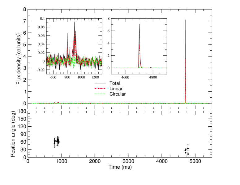
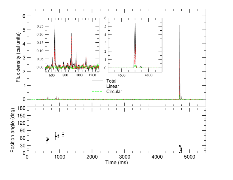
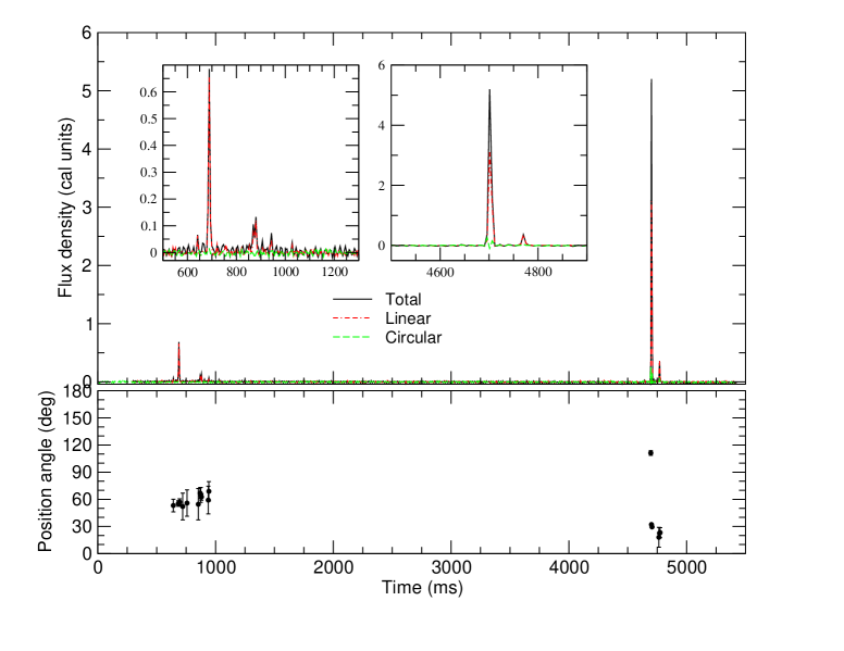
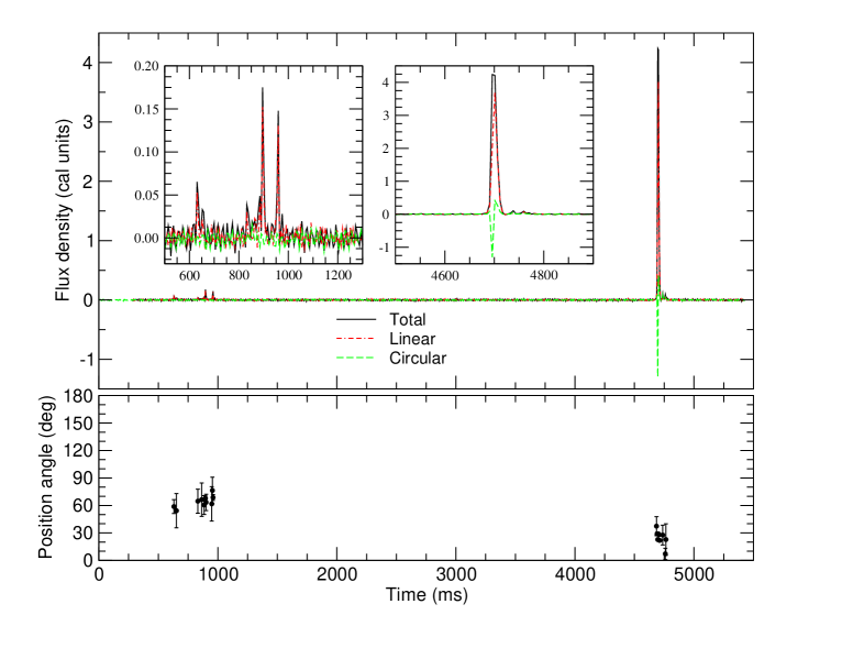
Figure 1: The four strongest pulses as measured during session 3 at 8.4 GHz in full polarization. Insets shown enlarged regions of the MP (left) and IP (right). In all cases, the components in the IP region (around time 4800 ms) shows stronger emission than those in the MP region (around time 1000 ms) as also found for the next six strongest pulses. Note the large degree of circularly polarized emission seen with different handedness.

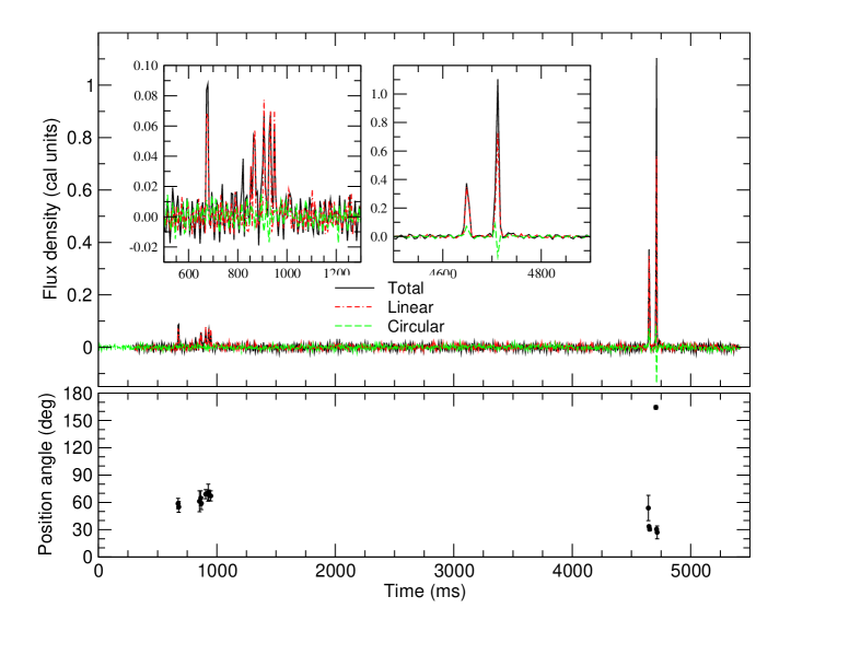
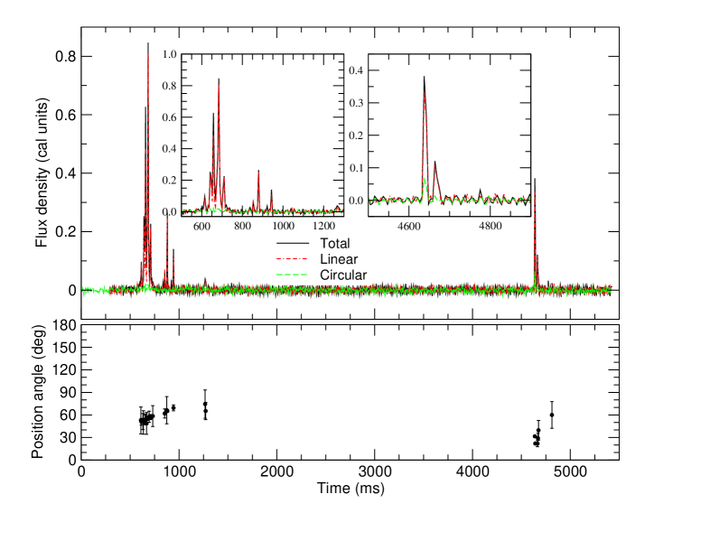
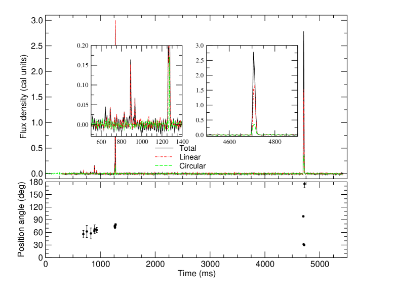
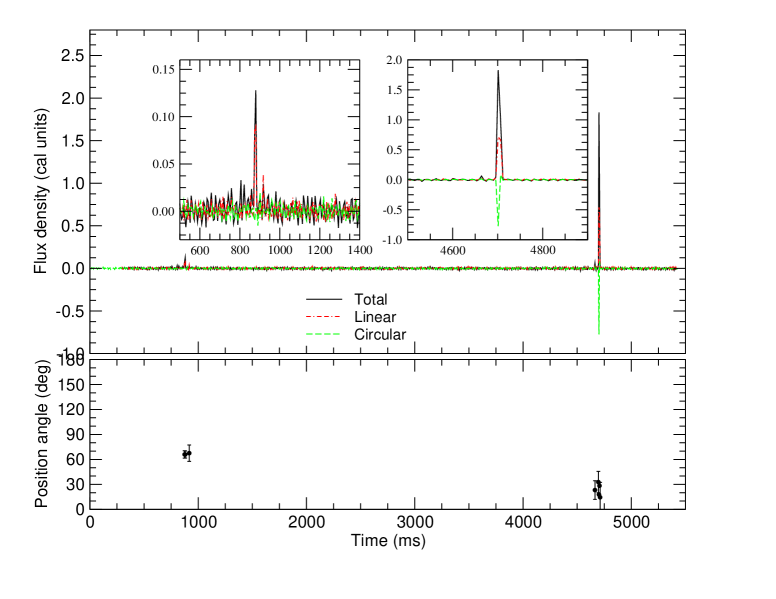
Figure 2: A sample of further pulses from the same data set used for the previous figure, demonstrating the wider variety of pulses appearing at pulse phases forming the MP. Note that the MP is nearly 100% linearly polarized while the IP shows some strong circular polarization of changing handedness.

3.2 Average pulse shapes at multiple frequencies

The variation of the integrated pulse shape on very short time scales as reported by Camilo et al. (2006b) is also visible in our data. While the total power profile changes, the degree of linear polarization remains extremely high. At the same time, changes in circular polarization in both degree of polarization and handedness are observed on short and long time scales. The average position angle swing is typically stable over the time scale of days, but we do detect different (non-orthogonal) polarization modes which modify this statement to some extent (see below).

In Figure 3, we present the polarization of the pulse profile observed at various frequencies during the observing sessions. We also include multi-frequency data that are observed only quasi-simultaneously (i.e. within periods of a few hours) as we find that the polarization features are much more persistent than the total power profiles which change on time-scales of 10 minutes (cf. Camilo 2006b). The properties of single pulses seen simultaneously at different frequencies will be discussed in a forthcoming paper.

In the first session (Fig. 3a), the source was very strong at all frequencies and single pulses were easily detected. No polarisation is available in this session at 1.4 GHz. The profile shows significant evolution with frequency, such that the trailing MP components become more distinct towards 8.4 GHz. Significant left-handed circular polarization is detected under the strong peak consistently at 4.9 GHz and 8.4 GHz, while the linear polarization exceeds 90%. The position angle is identical at the different frequencies, showing deviations from a smooth curve by exhibiting a deep ’dip’ at the longitude apparently separating the first and second components.

In general the swing does not follow a S-like curve as would be expected in a rotating vector model [Radhakrishnan & Cooke 1969] but is rather shallow. The average slope is rather modest, $d\Psi/d\Phi=1$ deg/deg covering only 45 deg in PA over the whole MP emission window. The steepest slope is measured during session 1 in the leading pulse component with a value of $d\Psi/d\Phi=3.5$ deg/deg. As we will discuss later in some detail, the PA swing of the IP changes between observing sessions but typically shows a larger, negative slope.

In the second observing session (Fig. 3b), the frequency evolution of the pulses occurring at the MP is much stronger with the greatest complexity exhibited at the highest frequencies. Remarkably, the IP was not detected at 1.4 GHz but appeared clearly at 8.4 GHz. This trend is repeated during the third session (Figure 3c), where the IP goes from just barely detectable at 1.4 GHz to become the dominant component at 8.4 GHz, indicating a much flatter spectrum of the IP relative to the MP. Where detected, the IP shows consistently significant left-handed circular polarization, but the degree of linear polarization is less than in the MP which remains more than 90% linearly polarized. Circular polarization of the same sense is weak but still detected at 1.4 GHz under the leading MP component, while the later MP components are stronger at higher frequencies, allowing the detection of circular polarization of the opposite sense. The PA swing has significantly changed from the first observations. This change is discussed in detail in the next section.

During session 5, the IP is still very weak at 1.4 GHz, but in sessions 7 and 8 (Figure 3e,f) the MP and IP are essentially of similar strength at all frequencies. Still, this should not be taken as a sign that the MP is becoming stronger with time. Instead, it demonstrates the significant time variability of the IP and its spectrum in particular. In any case, while the general polarization characteristics of the IP have not changed, the PA swing is now significantly different. Interestingly, the circular polarization that is clearly detected in the MP at 4.9 and 8.4 GHz appears to be predominately left-handed, but both frequencies consistently show a sense-reversal from right-hand to left-hand under the IP.

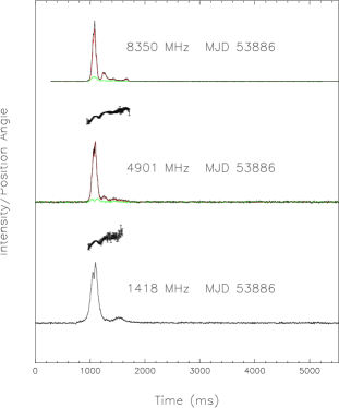
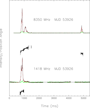
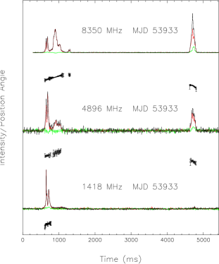
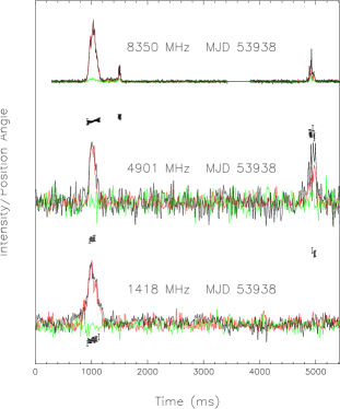
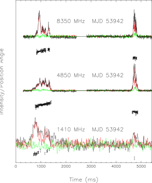
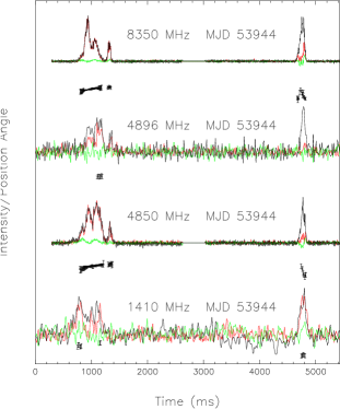
Figure 3: Average pulse profiles in full polarization observed at different frequencies for observing sessions 1,2,3,5,7 and 8. Total power (black) and linearly (red) and circularly (green) polarized power are shown together with the measured position angle for each epoch and frequency. The scale of the shown position angle swing is identical for all pulse profiles of a given epoch and presented here only to allow for a comparison of its general shape and extent. A quantitative comparison is made in Figures 7 and 8.

3.3 Average pulse profiles at multiple epochs

In order to study the siginificant pulse shape changes in more detail with respect to the polarization properties, we present these with additional pulse profiles measured at 4.9 GHz and 8.4 GHz in Figure 4 over a period of several weeks.

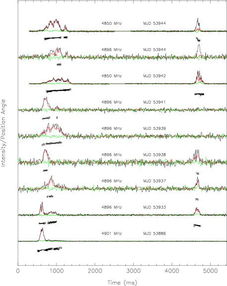
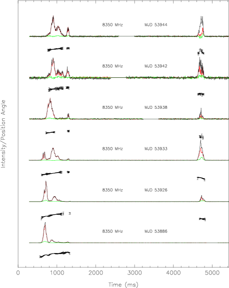
Figure 4: Comparison of the average pulse profiles in full polarization observed over several weeks at 4.9 GHz and 8.4 GHz. Total power (black) and linearly (red) and circularly (green) polarized power are shown together with the measured position angle for each epoch and frequency. The scale of the shown position angle swing is again identical for all pulse profiles of a given epoch and presented here only to allow for a comparison of its general shape and extent. A quantitative comparison is made in Figures 7 and 8.

The most striking feature in both plots is clearly the coming and going of certain emission components with time. Moreover, while the MP stays essentially completely linearly polarized, the circular polarization remains low but mostly left-handed in the strong MP components. In contrast, the circular polarization in the IP is changing handedness, reflecting the variation seen in the individual pulses. Moreover, the IP shows a typically much smaller degree of polarization in general, with the PA swing clearly changing slope and shape. It is also notable that the MP component that was clearly dominant in the early observing session has disappeared towards the later epochs.

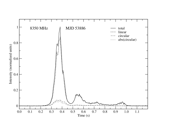
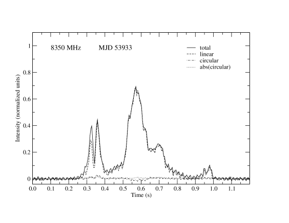
Figure 5: Polarization of main pulse as measured at 8.4 GHz during sessions 1 and 3. The leading component which disappears toward the later epochs is less linearly polarized than the trailing components. It also shows a significant amount of circular polarization which becomes weaker at later epochs. The degrees of polarization for these two epochs are (total: $89.4\pm 0.2$%, linear: $88.8\pm 0.2$%, circular: $10.9\pm 0.1$%, absolute circular: $10.4\pm 0.1$%) and (total: $92.8\pm 0.7$%, linear: $92.6\pm 0.7$%, circular: $0.8\pm 0.4$%, absolute circular: $1.7\pm 0.2$%), respectively. Corresponding values observed at the lower frequencies are consistent.

Inspecting the polarization properties in detail, one notices that the first component of the main pulse is less polarized than the later components (see Figure 5 and caption). As we will see further on, this is a region where a larger variety of position angles are observed, but it also conincides with a region of significant amount of average circular polarization. It is then interesting to note that the degree of circular polarization is almost identical to the amount obtained when adding the absolute value of circular intensity to form the average profile. That indicates that the variety of circular polarization seen in the spiky single pulses for a wide range of pulse phases essentially cancels out and only a lower level of persistent circular polarization remains. At later epochs, this first component seems to gradually disappear, and the only highly linearly polarized components remain.

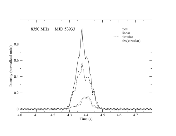
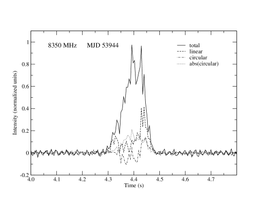
Figure 6: Polarization of interpulse as measured at 8.4 GHz during sessions 3 and 8. Significant amounts of positive circular is seen during the first epoch, while the circular intensity is more structured and with sense reversal during the later epoch. The degrees of polarization for these two epochs are (total: $69.8\pm 0.5$%, linear: $68.1\pm 0.5$%, circular: $16.0\pm 0.3$%, absolute circular: $16.0\pm 0.3$%), (total: $27.6\pm 1.0$%, linear: $26.2\pm 1.1$%, circular: $0.0\pm 1.0$%, absolute circular: $8.9\pm 0.7$%), respectively. Corresponding values observed at the lower frequencies are consistent.

The situation is somewhat different for the interpulse, which is significantly less polarized than the main pulse (see Figure 6 and caption). A variety of circularly polarized single pulses leaves a significant but changing degree of circular polarization. This conincides with a lower degree of linear polarization with a large variety of position angle values.

3.4 Position angle swings

Despite the striking changes in average pulse profiles presented above, the PA swing in the MP is changing much less dramatically and in a more organized fashion. The situation is quite different for the IP. In order to verify that the PA changes seen in the MP are a function of time, rather than observing frequency, we first compare the PA swings seen simultaneously at different frequencies. In Figure 7 we plot the PA at longitudes where the linear polarized emission is strong enough to exceed a signal-to-noise ratio threshold of 4. The agreement between the different frequencies is extremely good, demonstrating the general broad-band character of the PA swing, while simultaneously validating our calibration procedures. Note that the agreement is found for both the MP and IP, with the only exception being the IP data measured at 1.4 GHz during session 8.

Having calibrated the absolute position angles for both 4.9 GHz and 8.4 GHz, we use a measured offset of $\Delta PA=-10^{\circ}\pm 2^{\circ}$ to infer a rotation measure of RM$=+71\pm 14$ rad m^-2.

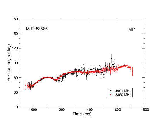
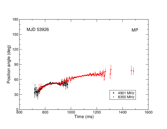
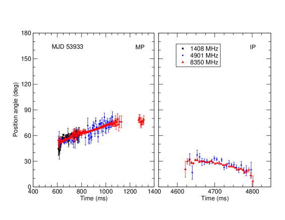
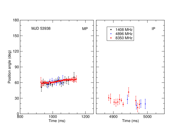
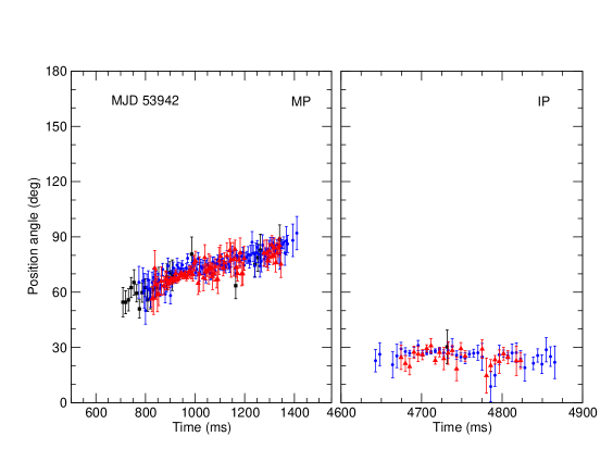
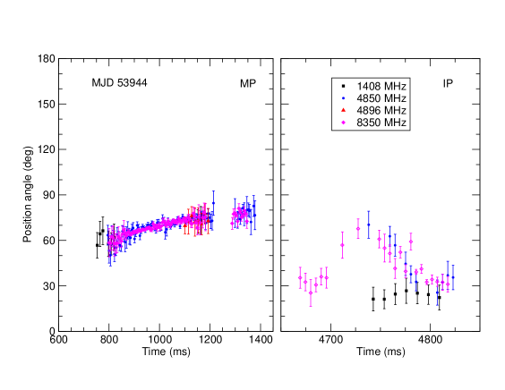
Figure 7: Position angle swing of the linearly polarized components observed at different frequencies for several observing sessions, namely 1, 2, 3, 5, 7 and 8.

As was evident from a comparison of the PA swings in Figure 3, the PA changed between the observing sessions. In Figure 8, we show the evolution of the PA as a function of time in more detail for both the MP and IP as measured for 4.9 GHz and 8.4 GHz. For reasons of clarity, we have offset the PA swings to each other by a fixed amount which is the same each for both the MP and IP. A clear trend is visible where the previously discussed dip becomes less prominent from session 1 to session 2 before it has disappeared at session 5. Interestingly, the longitude range where the dip was present is later replaced by PA values which show a significant scatter, typically much larger than at other pulse longitudes. A slight change in the overall slope is also visible. The figure also demonstrates again how the leading MP component disappears with time, while the most trailing component of the MP remains essentially detectable at all times, at least at 8.4 GHz. Surprisingly, observations at both frequencies with both Effelsberg and Westerbork show an interesting ’wiggle’ or oscillation in parts of the PA swing which follows the longitudes of the ’dip’ seen in session 1.

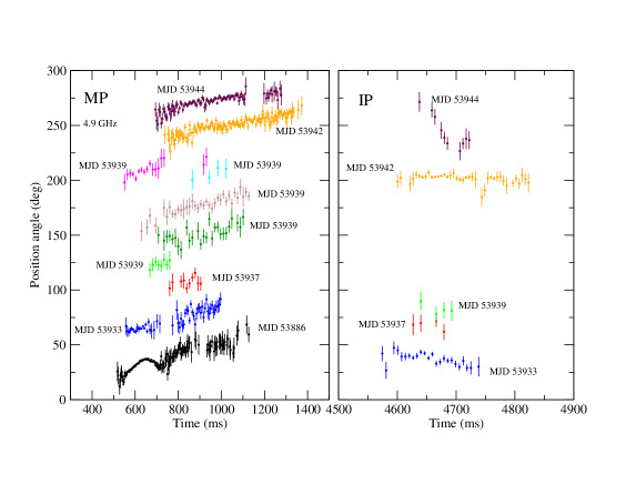
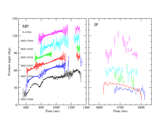
Figure 8: Position angle swing as measured at 4850 MHz and 8350 MHz as a function time for the MP and IP components.

When studying the evolution of the PA swing measured in the IP, it is obvious that it changes significantly with time. In addition to obvious changes in the swing, it is remarkable that it also changes in absolute PA value. This is notable by comparing the separation of the PA values measured at different days and relating this to the fixed offset introduced to the PA curves and visible in the MP plots. As the PA swings in the MP components agree perfectly as shown above, this variation in absolute PA is clearly intrinsic to the source. A possible explanation for this effect is obtained when considering the existence of polarization modes.

3.5 Polarization modes

Normal radio pulsars are known to exhibit linear polarisation modes which are typically orthogonal to each other. The origin of these so-called orthogonal modes (e.g. Backer et al. 1976) is believed to be related to mode-separating birefringence effects in the pulsar magnetosphere (McKinnon 1997, Petrova 2001). Simultaneous multi-frequency observations found (Karastergiou et al. 2002) that there is a high degree of correlation between the polarization modes at two different frequencies. They also found that the modes occur more equally towards higher frequencies, providing some explanation for the de-polarization of pulsar emission at high frequencies, as overlapping orthogonal modes lead to a lower average degree of polarization.

The extremely high degree of polarization seen at all frequencies for AXP J1810$-$197  would suggest that different orthogonal modes should not be present as they often lead to a de-polarization of the average pulse profiles (McKinnon 1997, Karastergiou et al. 2002). In order to verify this expectation, we studied the distribution of PAs for each phase bin. To avoid spurious contributions, we only registered those signals where both the total and linear intensity were 6 times stronger than the corresponding off-pulse RMS. The resultant PA histograms for three epochs are plotted in Figure 9 where we concentrate on the highest S/N data, i.e. frequencies of 4.9 GHz and 8.4 GHz.

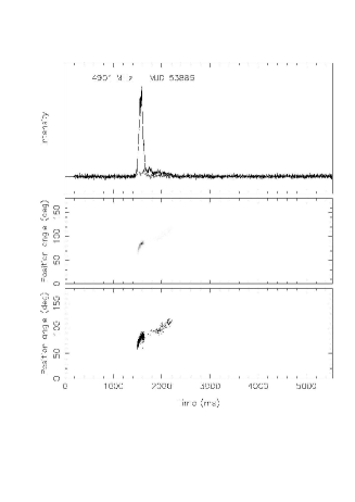
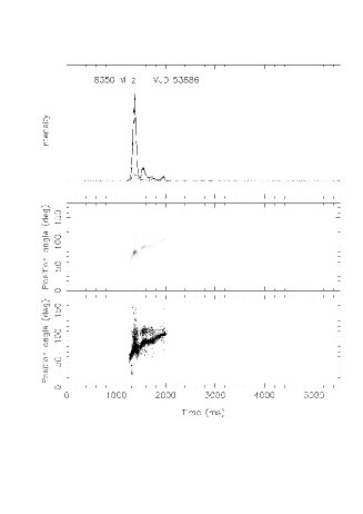
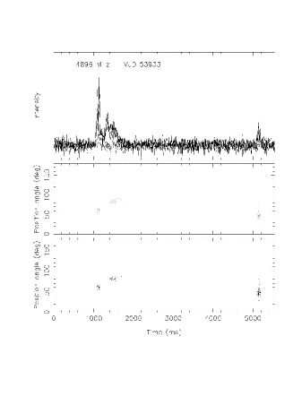
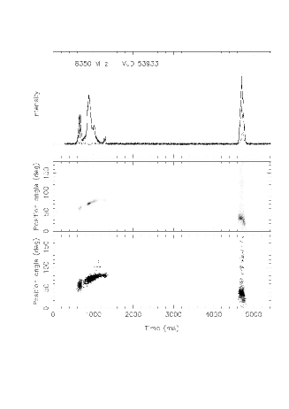
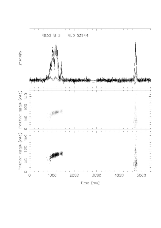
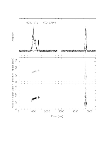
Figure 9: Distribution of occurrence of the position angles of the linearly polarized components measured at 4.9 GHz and 8.4 GHz for individual pulses during sessions 1, 3 and 8. The top panel in each plot shows the average pulse profile with linear and circular intensity. The middle plot indicates how often a particular PA value was measured per phase bin, using a intensity scale where dark regions mark the highest occurrences. The MP and IP regions were scaled independently, so that the darkest shades of gray correspond to the most frequently measured PAs in each region respectively. The bottom plot shows a scatter plot, indicating simply the measured PA value, irrespective of the frequency of occurrence.

For each epoch and frequency, we show two PA plots. The bottom plot shows a scatter plot, indicating simply the measured PA values, irrespective of the frequency of occurrence. The middle plot shows instead how often a particular PA value was measured per phase bin, using a gray-scale plot. The darkest regions mark the highest occurrences of PA. The MP and IP regions were scaled independently, so that the darkest shades of gray correspond to the most frequently measured PAs in each region respectively.

In the histogram for session 1 at 8.4 GHz, one can see two well separated regions of highly populated PA values indicating the existence of two polarization modes. The two observed modes are non-orthogonal and are present at nearly all pulse longitudes - apart from the ’dip’ region where only one mode seems to be present. The reason why this mode separation does not lead to a complete de-polarization of the average profile becomes clear when studying the middle panel, which reflects the occurrence of the PA values. While the existence of the two modes is highly significant, the second mode does not occur very frequently. Interestingly, studying the PA values at 4.9 GHz, the second mode is not visible despite this data set covering a longer time span, containing 1437 pulses, compared to 972 pulses obtained at the higher frequency. In contrast, it is important to note that the average pulse profiles at both frequencies are in perfect agreement. The fact that we also observe circular polarization in the same pulse longitude range may therefore indicate that we observe a conversion from linear into circular power at high frequencies as the result of a propagation effect.

The occurrence of a second polarization mode seen in the MP is also changing between observing session. In the histograms shown for session 3, the MP polarization is essentially confined to one mode and the spread within this mode is also smaller. However, in contrast, the polarization under the IP shows an extremely large scatter in the PA swing. On the one hand, a very wide range of PA values occurs as seen in the bottom panels. On the other hand, even though PA values that differ greatly from the average PA are not very common (see middle panels) the scatter around the average values is still quite large. This explains why the shape and absolute angle of the IP seem to change with time as the average IP properties then depend on the particular single pulses added in the IP region. Although the signal-to-noise ratio at 4.9 GHz is worse than at 8.4 GHz, an identical behaviour is clearly seen at both frequencies.

The third epoch shown Figure 9 is one where the ’wiggle’ in the PA swing discussed earlier are very clearly seen. And indeed, both the scatter plot as well as the PA density plot clearly indicate a spread and almost bimodal distribution in the corresponding pulse phase range. The regularity of the wiggle variation is quite striking and may suggest the existence of propagation effects in the magnetosphere that can change the ratio of Stokes $Q$ and $U$ in a systematic way as a function of pulse longitude.

The occurrence of significantly different PA values in the IP region is also seen at all epochs and explains why we find it difficult to fit an acceptable rotating vector model [Radhakrishnan & Cooke 1969] to both the MP and IP polarization data. Such a fit can in principle produce a value for the magnetic inclination angle $\alpha$ and the impact angle of the line-of-sight to the magnetic pole $\beta$ (e.g. Lyne & Smith 2006). A number of models, including wide cones and dual pole models with and without orthogonal jumps between the IP and MP were tried and no simultaneous fit to both sets of PAs were possible at any frequency. Instead, one can find independent fits to the MP and IP where at least the viewing angle, i.e.  the angle between the rotation axis and the line-of-sight, are consistent. An example for such a solution is shown in Figure 10 for the 8.4 GHz data of session 3. Here we find for the MP data a solution ($\alpha=44^{\circ}\pm 1^{c}irc$, $\beta=39^{\circ}\pm 4^{\circ}$) and for the IP ($\alpha=76.6^{\circ}\pm 0.2^{\circ}$, $\beta=6^{\circ}\pm 4^{\circ}$). As indicated, both solutions have an identical value for $\alpha+\beta=83^{\circ}$. We discuss the interpretation of this solution further below.

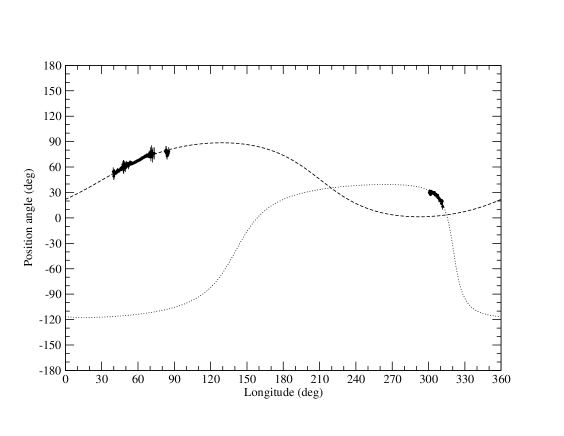
Figure 10: Rotating vector model fits for the 8.4-GHz data measured in session 3. Two separate rotating vector models are fitted to the MP and IP separately as no acceptable solution exists for a simultaneous fit. The fits shown produce an identical viewing angle of $\alpha+\beta=83^{\circ}$.

3.6 Stability of polarization

As indicated earlier, apart from a long-term evolution of the pulsar profile and its polarization properties, we also see short-term variations, including variations in the circularly polarized emission component. In Fig. 11 we show an example of WSRT data taken during session 3 over a period of 6 hours. While the circular polarization of the IP region seems to be unchanged within the uncertainties, the circular polarization in the MP shows changes from negative to positive handedness. A similar behaviour is also seen on long time-scales with the MP showing changes even though the average degree of circular polarization remains low and mostly positive. In contrast, the IP tends to be more stable in circular polarization but in particular in the later sessions stronger variations are observed (see Fig. 3).

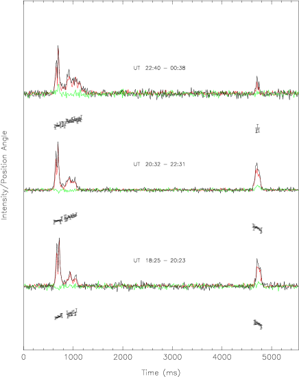
Figure 11: Example of short-time variation in the circular polarization of the average pulse profile. The shown observations were recorded at 4896 MHz in the night from MJD 53933 to 53934. Each profile corresponds to about 120 min of integration time. The change in the handedness of the circular polarisation in the MP is clearly visible. At the same time, the circular polarization in the IP remains essentially unchnaged.

4 Discussion

It is clear that the radio emission of AXP J1810$-$197 shows several features observed in ordinary radio pulsars, but also shows a large variety of striking and peculiar differences. Among the most striking differences are probably the flat spectrum of AXP J1810$-$197 , making it an extraordinarily strong source at high radio frequencies, and the constantly changing, extremely highly polarized pulse profile.

In normal radio pulsars, the addition of several hundred pulses is usually sufficient to reach a stable pulse profile (Helfand et al. 1975, Rankin & Rathnasree 1995). On short time-scales of the order of minutes to hours, changes are sometimes seen as a phenomenon known as mode-changing (Backer 1970) in which the pulsar switches between a small number of (typically two) stable pulse profiles. The dramatic changes between a large variety of pulse shapes on time-scales ranging from minutes to weeks as seen in AXP J1810$-$197 are clearly unusual. Perhaps, this source does not exhibit a stable pulse shape as such, or the stabilization time-scale is extremely large. The latter would indeed be consistent with the extreme narrowness of the very spiky single pulses being observed.

Indeed, rather than having broad sub-pulses as typically seen in normal pulses, the spiky pulses occur at seemingly random positions within the range of pulse phases for which emission is detected in the average pulse profile. Such spiky emission is only rarely observed in normal pulsars, but when it is observed it also leads to very long profile stabilization time-scales. Weltevrede et al. (2006b) observe a time-scale of over 25,000 pulses for PSR B0656+14 at 327 MHz. Scaling this time-scale to the period of AXP J1810$-$197 , this would imply a required observing time of about 38 hours to reach a stable pulse profile. This is much longer than the time taken to obtain any of the profiles presented so far in this paper or by other authors, making this possibility a plausible explanation. On the other hand, the range of pulse phases for which emission is detected also changes systematically over timescales of weeks, with the first component apparently slowly disappearing at later epochs. This may indicate that the situation is more complex and that a stable pulse profile may indeed be nonexistent in the first place.

The spiky appearance of the single pulses of AXP J1810$-$197 is more reminiscent of the narrow ’giant micropulses’ found first for the Vela pulsar (Johnston et al. 2001) and later for a few others (Johnston & Romani 2002). These giant micropulses tend to occur at the edges of pulse profiles, in contrast to the wide variety of pulse phases for which the spiky pulses of AXP J1810$-$197 are seen. Moreover, pulsars with giant micropulses often have relatively large magnetic fields near the light cylinder, similar to pulsars exhibiting ’real’ giant pulses (see e.g. Lorimer & Kramer 2005). In contrast, the magnetic field at the light cylinder of AXP J1810$-$197 , as inferred from the observed period and spin-down, is only about 14 Gauss – several orders of magnitudes lower than those estimated for Vela or the Crab pulsar. Even though the evidence for the connection between the detection of giant pulses and a strong light-cylinder magnetic field is somewhat circumstantial, it suggests that the emission mechanism creating giant pulses may not be directly related to that creating the radio emission of AXP J1810$-$197 . However, it is plausible that the pulses from AXP J1810$-$197 originate from a much lower height in the magnetosphere where similar conditions, in particular larger magnetic field strengths, would be encountered. Unfortunately, we know little about the emission properties of RRATS (e.g. their polarization properties) at the moment to allow for a similar, meaningful comparison with these sources. It will be intriguing to see whether the hypothesis that RRATS provide a link between radio pulsars and magnetars (McLaughlin et al. 2006) is confirmed by finding similar emission properties to be determined in future RRATS studies.

While the total power pulse profiles differ significantly between the frequencies, the same applies to the linearly polarized components, as the degree of polarization typically exceeds 90% at most MP longitudes, following the total power profile closely. In contrast, the degree of linear polarization for the leading MP component is lower and significant amounts for circular polarization are observed. For the rest of the MP the degree of circular polarization remains low. Some changes are observed but as far as it can be deduced from the generally much lower signal-to-noise ratio they are much less dramatic than those of the linear or total power profile.

Apart from a clear evolution over a timescale of weeks, one of the most stable features in the pulse profile is the PA swing of the MP. There is also excellent agreement between the PA seen at different frequencies when detected at the same pulse longitudes. This agreement appears to be even better than the general good agreement found for pulsars by Karastergiou & Johnston (2006).

If the PA swing is interpreted geometrically as in the rotating-vector-model, a change in the PA should only occur if either the geometry is changing (e.g. due to precessional effects) or if the underlying magnetic field structure is undergoing changes. Stability of the magnetic field structure is usually considered to be a safe assumption for radio pulsars where the long-term stability of the average pulse profile and its position angle swing is attributed to the dominance and strength of the dipolar magnetic field (e.g. Manchester & Taylor 1977). Even though the PA swing of normal pulsars often shows deviations from an S-like shape (Lyne & Manchester 1988) and sometimes exhibits some variation across frequencies, this is often attributed to the existence of orthogonal emission modes and their different spectral properties (Karastergiou & Johnston 2005). The long-term evolution of PA swing in the MP of AXP J1810$-$197 is therefore highly unusual. The clear trend seen over timescales of days and weeks suggests that this is a relatively slow process. Distinguishing between the possibilities as to whether this is related to changes in the magnetic field structure, or to precessional effects, or to the fact that the PA swing is not reflecting the geometry of the system after all and that propagation effects in the magnetosphere or non-dipolar field components are involved, is difficult. However, there are a number of observed properties which indeed suggest the existence of severe propagation effects in the magnetosphere: (a) we see distinct polarization modes which change with radio frequency and time; (b) we see a large variety of PA values in the IP region; (c) we have indications of a conversion of linear into circular power for certain pulse longitude ranges (d) we see interesting wiggles in the PA slopes which are hard to explain by a any geometrical model and (e) even the changing flux density spectrum of the individual MP and IP components could be due to propagation effects. Indeed, the magnetosphere is much larger than that of a typical radio pulsar, and the range of inferred magnetic field strengths encountered from the surface ($B=2.6\times 10^{14}$ Gauss) to the light-cylinder ($B=14$ Gauss) is certainly enormous, covering 13 orders of magnitude and hence giving scope for a large variety of effects.

Despite the likelihood of magnetospheric propagation effects, it is tempting to associate the deviations from an S-like swing (and the inability to find a single set of rotating-vector-model parameters that connects both the MP and IP with a satisfactory fit) with deviations from a dipolar field structure. We also note that the separation of the IP from the MP is quite different from the 180 deg expected in a two-pole model, and that the emission properties of the IP are rather different from those of the MP, supporting the interpretation of detecting signatures of non-dipolar field lines. Indeed, within the magnetar model a dipolar field structure is not necessarily expected. Similar arguments have been put forward to explain some of the polarization and profile properties of millisecond pulsars (e.g. Xilouris et al. 1998) where the evolutionary history of the sources may lead to non-dipolar and sun-spot-like field structures (Ruderman 1991). However, depending on the emission height and hence the physical separation from the field’s multipole components, their actual impact in the emission region may actually be low, although they may affect the plasma flow from the surface and hence the observed radio properties.

The relative shallowness of the PA swing under the MP with a slope of only 1 deg/deg is not uncommon for pulsars whereas the PA evolution with epoch certainly is. It is interesting to compare the properties of AXP J1810$-$197 with those of young pulsars, as the characteristic age of AXP J1810$-$197 is less than 10,000 years. Johnston & Weisberg (2006) studied 14 young pulsars with characteristic ages less than 75 kyr and found that generally pulse profiles are simple and consist of either one or two prominent components whereas the linearly polarized fraction is nearly always in excess of 70 per cent. The latter characteristic is certainly true for AXP J1810$-$197 but the profile is clearly anything but simple, nor does the trailing component dominate, as Weisberg & Johnston (2006) also find, on average, for young pulsars.

The flat PA curve could be both explained either by an aligned configuration in which the spin-axis is aligned with the magnetic field axis, or by a very wide cone which is cut far away from the magnetic pole. The solution for the RVM fits to the MP presented in Section 3.5 corresponds to an extremely wide cone grazed at the outside for the MP ($\alpha=44^{\circ}$, $\beta=39^{\circ}$), with a beam radius inferred from the MP pulse width of about $\rho\sim 44^{\circ}$. (Note that both the MP and IP are not centred on the steepest gradient of the fitted RVM curves.) In contrast, the inferred beam radius for the IP is much smaller, $\rho\sim 8^{\circ}$. However, there are some hints of a correlation in strength between the IP and trailing MP components, so that one could consider both emission features as part of another wide cone. In comparison, the radio beam of normal radio pulsars appears to scale with $\propto 1/\sqrt{P}$, which would imply a beam radius for AXP J1810$-$197 of less than 3 deg when measured at a 50% intensity level (Lorimer & Kramer 2005). Alternatively, with an aligned configuration, the observer’s line-of-sight may hardly ever leave the emission cone, also creating a wide pulse width. In any case, if we interprete the RVM fits geometrically, then we have to conclude that we observe two emissions cones, that are centred on different independent magnetic poles separated by 109 degrees in neutron-star longitude. We can interprete that either as an offset dipole or evidence of a non-dipolar field configuration. The viewing geometry and the rather different emission properties of the various pulse components are certainly consistent with this view.

It is intriguing that AXP J1810$-$197 shows variations in its spin-down (Camilo et al. 2006b), which could be related to changes in the torque and hence the magnetic field structure near the light-cylinder. If these torque changes are related to the magnetic field structure changing near the light-cylinder, it may also show changes in the emission region. In the magnetar model (Duncan & Thompson 1992) one expects that changes in the magnetic field may trigger energetic outbursts. This seems to be inconsistent with the observation that no X-ray variation was seen in recent monitoring observations (Camilo et al. 2006b). However, Beloborodov & Thompson (2006) propose that a plasma corona forms around the neutron star, as a result of occasional starquakes that twist the external magnetic field of the star and induce electric currents in the closed magnetosphere. If such effect is present, one could speculate as to whether a combination of twisted fieldlines and changing plasma corona is responsible for the observed emission properties. Continuing studies of simultaneous multi-frequency data offer a chance to indeed separate changing geometrical/field-configuration effects from propagation effects. Further such studies are in progress and will be presented elsewhere.

5 Summary

We have observed the magnetar AXP J1810$-$197 in full polarisation using three different telescopes simultaneously at three different frequencies. We find that some properties of AXP J1810$-$197 ’s are similar to those of normal radio pulsars while many more features are observed that are strikingly different. We find strong evidence for propagation effects in the magnetosphere while the observed emission properties are consistent with a multi-pole configuration of the magnetic field. Continued observations of this radio emitting magnetar, together with the future studies of RRATS sources, will allow us to study a variety of neutron stars in the radio regime and to contrast their emission properties with those of normal pulsars.

References

- [Backer 1970] Backer D. C., 1970, Nature, 228, 1297
- [Backer, Rankin & Campbell 1976] Backer D. C., Rankin J. M., Campbell D. B., 1976, Nature, 263, 202
- [Beloborodov & Thompson 2006] Beloborodov A. M., Thompson C., 2006, in Isolated Neutron Stars: from the Interior to the Surface, astro-ph/0608372
- [Camilo et al. 2006b] Camilo F., Ransom S. M., Halpern J. P., Reynolds J., Helfand D. J., Zimmerman N., Sarkissian J., 2006a, Nature, 442, 892
- [Camilo et al. 2006a] Camilo F. et al., 2006b, submitted, astro-ph/0610685
- [Duncan & Thompson 1992] Duncan R. C., Thompson C., 1992, ApJ, 392, L9
- [Edwards & Stappers 2004] Edwards R. T., Stappers B. W., 2004, A&A, 421, 681
- [Gould & Lyne 1998] Gould D. M., Lyne A. G., 1998, MNRAS, 301, 235
- [Halpern et al. 2005] Halpern J. P., Gotthelf E. V., Becker R. H., Helfand D. J., White R. L., 2005, ApJ, 632, L29
- [Helfand, Manchester & Taylor 1975] Helfand D. J., Manchester R. N., Taylor J. H., 1975, ApJ, 198, 661
- [Ibrahim et al. 2004] Ibrahim A. I. et al., 2004, ApJ, 609, L21
- [Johnston & Romani 2002] Johnston S., Romani R., 2002, MNRAS, 332, 109
- [Johnston & Weisberg 2006] Johnston S., Weisberg J. M., 2006, MNRAS, 368, 1856
- [Johnston, Karastergiou & Willett 2006] Johnston S., Karastergiou A., Willett K., 2006, MNRAS, 369, 1916
- [Johnston et al. 2001] Johnston S., van Straten W., Kramer M., Bailes M., 2001, ApJ, 549, L101
- [Karastergiou & Johnston 2006] Karastergiou A., Johnston S., 2006, MNRAS, 365, 353
- [Karastergiou, Johnston & Kramer 2003] Karastergiou A., Johnston S., Kramer M., 2003, A&A, 404, 325
- [Karastergiou et al. 2001] Karastergiou A. et al., 2001, A&A, 379, 270
- [Karastergiou et al. 2002] Karastergiou A., Kramer M., Johnston S., Lyne A. G., Bhat N. D. R., Gupta Y., 2002, A&A, 391, 247
- [Kaspi & McLaughlin 2005] Kaspi V. M., McLaughlin M. A., 2005, ApJ, 618
- [Lorimer & Xilouris 2000] Lorimer D. R., Xilouris K. M., 2000, ApJ, 545, 385
- [Lorimer, D. R. and Kramer, M. 2005] Lorimer, D. R. and Kramer, M., 2005, Handbook of Pulsar Astronomy. Cambridge University Press
- [Lorimer et al. 1998] Lorimer D. R., Jessner A., Seiradakis J. H., Lyne A. G., D’Amico N., Athanasopoulos A. Xilouris K. M., Kramer M., Wielebinski R., 1998, A&AS, 128, 541
- [Lyne & Graham-Smith 2006] Lyne A. G., Graham-Smith F., 2006, Pulsar astronomy, Cambridge University Press, Cambridge
- [Lyne & Manchester 1988] Lyne A. G., Manchester R. N., 1988, MNRAS, 234, 477
- [Manchester & Taylor 1977] Manchester R. N., Taylor J. H., 1977, Pulsars. Freeman, San Francisco
- [McKinnon 1997] McKinnon M., 1997, ApJ, 475, 763
- [McLaughlin et al. 2003] McLaughlin M. A. et al., 2003, ApJ, 591, L135
- [McLaughlin et al. 2006] McLaughlin M. A. et al., 2006, Nature, 439, 817
- [Mitra et al. 2003] Mitra D., Wielebinski R., Kramer M., Jessner A., 2003, A&A, 398, 993
- [Petrova 2001] Petrova S. A., 2001, A&A, 378, 883
- [Radhakrishnan & Cooke 1969] Radhakrishnan V., Cooke D. J., 1969, Astrophys. Lett., 3, 225
- [Rankin & Rathnasree 1995] Rankin J. M., Rathnasree N., 1995, ApJ, 452, 814
- [Ruderman 1991] Ruderman M., 1991, ApJ, 366, 261
- [Shitov, Pugachev & Kutuzov 2000] Shitov Y. P., Pugachev V. D., Kutuzov S. M., 2000, in Kramer M., Wex N., Wielebinski R., eds, Pulsar Astronomy - 2000 and Beyond, IAU Colloquium 177. Astronomical Society of the Pacific, San Francisco, p. 685
- [van Leeuwen et al. 2003] van Leeuwen A. G. J., Stappers B. W., Ramachandran R., Rankin J. M., 2003, A&A, 399, 223
- [Voûte et al. 2002] Voûte J. L. L., Kouwenhoven M. L. A., van Haren P. C., Langerak J. J., Stappers B. W., Driesens D., Ramachandran R., Beijaard T. D., 2002, A&A, 385, 733
- [von Hoensbroech & Xilouris 1997] von Hoensbroech A., Xilouris K. M., 1997, A&AS, 126, 121
- [Weltevrede et al. 2006a] Weltevrede P., Stappers B. W., Rankin J. M., Wright G. A. E., 2006a, ApJ, 645, L149
- [Weltevrede et al. 2006b] Weltevrede P., Wright G. A. E., Stappers B. W., Rankin J. M., 2006b, A&A, 458, 269
- [Woods & Thompson 2006] Woods P. M., Thompson C., 2006, in Compact stellar X-ray sources, Eds. Walter Lewin & Michiel van der Klis, Cambridge University Press, Cambridge, p. 547 - 586
- [Xilouris et al. 1998] Xilouris K. M., Kramer M., Jessner A., et al., 1998, ApJ, 501, 286