CRATES: An All-Sky Survey of Flat-Spectrum Radio Sources

Abstract

We have assembled an 8.4 GHz survey of bright, flat-spectrum ($\alpha>-0.5$) radio sources with nearly uniform extragalactic ($|b|>10^{\circ}$) coverage for sources brighter than $S_{4.8\mathrm{\>GHz}}=65$ mJy. The catalog is assembled from existing observations (especially CLASS and the Wright et al. PMN-CA survey), augmented by reprocessing of archival VLA and ATCA data and by new observations to fill in coverage gaps. We refer to this program as CRATES, the Combined Radio All-sky Targeted Eight GHz Survey. The resulting catalog provides precise positions, sub-arcsecond structures, and spectral indices for some 11,000 sources. We describe the morphology and spectral index distribution of the sample and comment on the survey’s power to select several classes of interesting sources, especially high energy blazars. Comparison of CRATES with other high-frequency surveys also provides unique opportunities for identification of high-power radio sources.

1 Introduction

As extrema of the AGN population, blazars are of particular interest for a number of topics in accretion and jet physics. These sources are characterized by flat radio spectra; high variability, especially in the optical; significant polarization; and bimodal synchrotron/Compton SEDs. They are believed to be high-power radio AGN with a strong jet component viewed “pole-on.” For this model, Doppler boosting ensures that non-thermal jet emission will be strong. In cases where the non-thermal emission dominates the thermal flux from the accretion and surrounding broad-line region, the objects are known as HBL or BL Lacs. We are particularly interested in blazars since, at $\gamma$-ray energies, high-power blazars appear to dominate the observed EGRET sources (Hartman et al., 1999). The GeV Compton peak flux, in fact, likely dominates the cosmic background radiation at these energies. Similarly, the synchrotron IR-mm peak can dominate the point source contribution to the microwave sky (Giommi et al., 2006). Thus, large blazar surveys, probing the blazar population and its evolution, can be helpful for both $\gamma$-ray and microwave source identifications and for understanding cosmic backgrounds in these energy bands.

Flat-spectrum radio surveys are the prime source of blazar discoveries. Moreover, studies show that bright, flat-spectrum sources strongly correlate with sources in the $>$100 MeV sky (Mattox et al., 2001; Hartman et al., 1999; Sowards-Emmerd et al., 2005). In particular, our work has shown that high-energy associations are especially powerful when interferometric measurements of core flux density and spectral index are available. Further, since the “trough” between the blazar radio and $\gamma$-ray components lies in the optical to X-ray range, counterparts at these wavelengths are often faint. Indeed, many are known to have $R>23$, well below the sensitivity of the Second Digitized Sky Survey (DSS2). Positive identification is greatly helped by precise sub-arcsecond positions and structures, which require interferometric measurements at cm wavelengths.

Our survey is designed as an extension of the largest high-frequency interferometric survey currently available, the Cosmic Lens All-Sky Survey (CLASS) (Myers et al., 2003). We have replicated as closely as possible its selection criteria and extended the survey to the full sky at high Galactic latitudes through a combination of published data, reanalysis of archival data, and new observations. The product represents the largest sample of bright, compact, flat-spectrum sources available to date.

2 Sample Selection

2.1 Finding Sources

The basis for the CLASS sample selection was the GB6 catalog (Gregory et al., 1996) of sources in the declination range $0^{\circ}<\delta<+75^{\circ}$ measured at 4.85 GHz with the erstwhile 91 m telescope at Green Bank. In order to be observed as part of CLASS, a source had to lie outside the Galactic plane ($|b|>10^{\circ}$) and have a GB6 flux density of at least 30 mJy, at least one 1.4 GHz NVSS (Condon et al., 1998) source within $70\arcsec$ of the GB6 position, and a spectral index $\alpha>-0.5$ (where $S_{\nu}\propto\nu^{\alpha}$) computed between GB6 and NVSS. In the common case of multiple NVSS sources within $70\arcsec$ of a single GB6 position, the flux densities of the NVSS sources were added together, and this sum and the GB6 flux density were used to obtain the spectral index. All sources that satisfied these criteria were then observed interferometrically at 8.4 GHz with the VLA in the “A” configuration.

In order to produce a CLASS-like all-sky survey, we attempt to reproduce the CLASS selection criteria as closely as possible with the exception of the 4.8 GHz flux density threshold, which we increase to 65 mJy. Consequently, in the CLASS region itself ($0^{\circ}<\delta<+75^{\circ}$, $|b|>10^{\circ}$), CRATES is almost entirely a subset of CLASS.

Outside of the CLASS region, there are no GB6 observations, so it is necessary to introduce other catalogs as surrogates in order to select the sample. Single-dish observations of the southern sky at 4.85 GHz are available from the PMN survey catalog (Griffith & Wright, 1993), which covers the region $-87^{\circ}<\delta<+10^{\circ}$. Thus, below the equator, PMN serves as the parent survey for CRATES in the same way that GB6 serves for CLASS. To compensate for the different size of the dish used to conduct the PMN survey (the 64 m telescope at Parkes), we increase the matching radius for finding NVSS counterparts to $110\arcsec$. Further, NVSS observations are only available for $\delta>-40^{\circ}$, so below this declination, we substitute the 2006 June 1 version of the 843 MHz SUMSS catalog (Bock et al., 1999; Mauch et al., 2003) as our low-frequency survey for determining spectral indices. In this southernmost region of the sky, then, the sample selection is determined by PMN and SUMSS. Component matching in the low-frequency survey and the spectral index and flux density cuts are made to match the selection in the north.

GB6 is also unavailable in the north polar cap ($\delta>+75^{\circ}$), so sources there must be drawn from other high-frequency surveys. In this region, our prime source is the S5 catalog (Kühr et al., 1981) of sources in the range $+70^{\circ}<\delta<+90^{\circ}$ observed at 4.85 GHz with the Effelsberg 100 m telescope. This catalog is only complete to 250 mJy, so CRATES in the northern cap is considerably shallower than over the rest of the sky. NVSS does cover this region, though, so the CLASS-style matching procedure and spectral index cut can be applied to determine this part of the CRATES sample. A summary of this patchwork of surveys is shown in Table 1; in the rest of this paper, we will refer to the four sky regions by the names shown in the table.

Table 1: General characteristics of the CRATES sample.

Name of	Declination	4.85 GHz	4.85 GHz flux	Low frequency	Number of	Source density
sky region	range	survey	density depth	survey	sources	(number / $\sq^{\circ}$)
Far North	$+75^{\circ}<\delta<+90^{\circ}$	S5	250 mJy	NVSS (1.4 GHz)	79	0.111
North (CLASS region)	+00${}^{\circ}<\delta<+75^{\circ}$	GB6	65 mJy	NVSS (1.4 GHz)	4886	0.298
Equatorial South	$-40^{\circ}<\delta<$string$0^{\circ}$	PMN	65 mJy	NVSS (1.4 GHz)	4106	0.362
Far South	$-87^{\circ}<\delta<-40^{\circ}$	PMN	65 mJy	SUMSS (0.84 GHz)	2060	0.368

2.2 Uniformity of the Sample

In order to ensure that the CRATES sample selection is as uniform as possible, we must cross-calibrate the several surveys’ flux density measurements. Of course, the sources present in multiple surveys were not observed simultaneously, and blazars are significantly variable, so our cross-calibration can only be statistical. However, the mean flux density ratios give an estimate of any flux density scale offsets while the dispersions can be corrected for the measurement uncertainties to give an estimate of typical source variability. Additional variability estimates are also sometimes available from repeated observations within a given survey. For the 4.85 GHz catalogs, we identified common sources in the overlap zones. For example, GB6 and PMN overlap at $0^{\circ}<\delta<+10^{\circ}$, with $\sim$3000 common sources. The flux density ratio distribution shows that these surveys’ flux density scales are consistent within the expected statistical and variability fluctuations. Similarly, over 200 sources are common to the S5 and GB6 surveys; again, there is no significant offset. Thus, all 4.85 GHz selection is on a consistent flux density scale.

The situation is more complex for the low-frequency surveys used for spectral index selection. NVSS and SUMSS have a substantial overlap region ($-40^{\circ}<\delta<-30^{\circ}$) but are at quite different frequencies. Since we wish to select SUMSS sources that satisfy the $\alpha_{4.85/1.4}>-0.5$ cut, we must use the overlap sources to set an equivalent flux density/spectral index cut at 0.84 GHz. To set an appropriate threshold, we compare the PMN/NVSS and PMN/SUMSS spectral indices for $>$$10^{3}$ overlap sources as shown in Figure 1 along with a linear least squares fit. Clearly, the indices are not strictly proportional. The observed scatter is much larger than that due to flux density measurement errors and the observed high-frequency variability, so we infer a non-negligible curvature in the radio spectra that varies from object to object.

We accordingly estimate the equivalent 4.85 GHz/1.4 GHz spectral index as $\alpha_{4.85/1.4}^{\mathrm{equiv}}~{}=~{}A\alpha_{\mathrm{4.85/0.84}}~{}+~{}B$, where $\alpha_{4.85/0.84}$ is the observed PMN/SUMSS spectral indexand $A=1.143$ and $B=-0.105$ are the parameters of the fit. This transformation was performed for all PMN/SUMSS sources in the Far South.

Figure 1: Comparison of $\alpha_{4.85/0.84}$ and $\alpha_{4.85/1.4}$ spectral indices. The fit is $\alpha_{4.85/1.4}^{\mathrm{equiv}}=A\alpha_{\mathrm{4.85/0.84}}+B$, with $A=1.143$ and $B=-0.105$.

Applying the 4.85 GHz flux density cut, the $\alpha>-0.5$ spectral index cut (adjusted in the SUMSS region), and the Galactic plane cut, we obtained the final CRATES sample of 11,131 objects requiring X-band (8.4 GHz) measurements. An Aitoff equal-area projection of the sample is shown in Figure 2. Several features deserve comment. The source areal density is smaller in the Far North because of the shallower S5 survey. In the Equatorial South and Far South, the areal densities are larger than for the North (Table 1). This is apparently a consequence of the larger PMN 4.8 GHz beam, which will allow more extended and composite sources to pass the 65 mJy threshold. In addition, the presence of the Galactic bulge and the Magellanic clouds in the southern sky will introduce some thermal flat-spectrum, but extended, sources. Of course, composite and thermal sources will not be truly compact and will be unmasked by the 8.4 GHz interferometric observations. Indeed, there are more “no-shows” in the southern sky, and the final areal density of sources confirmed by our survey to be bright ($>$0.1 Jy at 8.4 GHz) is slightly higher in the North than in the two southern regions.

In addition, there are several holes in the 4.8 GHz samples in the Equatorial South and Far South, especially just south of $\delta=0^{\circ}$. We have used lower-frequency surveys to select nominally flat-spectrum radio candidates in these regions (see “Additional Observations” below) and have obtained X-band measurements, as resources permit, of the best sources. These sources may be promoted to full CRATES status by single dish 4.85 GHz observations. There is one obvious patch with a high density of flat-spectrum sources: this is the Large Magellanic Cloud (LMC), and much of the excess areal density is likely due to thermal sources in the LMC itself, but, of course, background blazars are present. The 8.4 GHz follow-up in this zone may be used to estimate the blazar fraction and to explore issues in extending CRATES to the Galactic plane region.

Figure 2: Aitoff equal-area projection of the CRATES sample in Galactic coordinates $(l,\,b)$. The central meridian is $l=0^{\circ}$. The concentration of points near $\delta=-70^{\circ}$ is due to sources in the Large Magellanic Cloud.

3 X-Band Observations

Fortunately, most of the required X-band observations are available in existing observatory archives. In particular, reduced measurements from CLASS at $0^{\circ}<\delta<75^{\circ}$ cover $>$99.5% of the CRATES-selected sources in this region. There are a few CLASS sources observed outside this declination range. The Equatorial South was surveyed for gravitational lenses in a manner very similar to CLASS using PMN/NVSS selection criteria very similar to CRATES (Winn et al., 2000). Thus, a substantial fraction of the required X-band observations was present in the VLA archives from a number of observing campaigns; we refer to these as CRATES-Va (VLA archive) below.

These data were remapped (and in some cases re-calibrated; see below), and measurements of component positions and flux densities were extracted for this survey. In the Far South, a significant source of archival observations was the (largely unpublished) PMN-CA survey (Wright et al., 1997); these were again remapped and remeasured for the present survey. A number of sources have also been measured in the AT 20 GHz (AT20G) Survey (Ricci et al., 2004; Sadler et al., 2006), which is still in progress. For the CRATES sample, we used a pre-release version of the AT20G catalog provided by the AT20G team and covering the declination region $-30^{\circ}$ to $-87^{\circ}$.

Some of these AT20G sources are also members of other sub-samples and helped to cross-calibrate the southern surveys. To complete CRATES, we have mounted several VLA campaigns, focusing on sources in the Far North and Equatorial South (program numbers AR0517 = CRATES-V1, AR0555 = CRATES-V2, AR0587 = CRATES-V3). Finally, we mounted an ATCA campaign (program C1468 = CRATES-CA) to observe the remaining sources south of $\delta=-40^{\circ}$. A handful of sources either ended up with only one ATCA scan or had SUMSS measurements published after our final observing campaign and thus missed being scheduled. The combination of the X-band data sets that we have collected provides $>$99.9% coverage of the CRATES targets.

3.1 New VLA and ATCA Campaigns

The three new VLA observational campaigns were each conducted with the VLA in the “A” array, using two 50 MHz bands at 8.44 GHz, but the observing schedule differed somewhat between runs. The first campaign, AR0517 (2003 July 23-25), targeted likely counterparts of southern 3EG $\gamma$-ray sources and is described in Sowards-Emmerd et al. (2004). The second campaign, AR0555, took place on 2004 October 2-3 and 2004 October 9. Here, some 1050 scans (duration 60-120 s) of over 900 sources were made. Standard AIPS calibration was performed followed by DIFMAP imaging and Gaussian component fitting. The final clean-up campaign, AR0587 (2006 March 22, 2006 April 1, and 2006 April 3), targeted some 282 survey sources plus frequent calibrator visits, obtaining $\geq$50 s on each. Again, standard mapping, calibration, and Gaussian component fitting were performed.

The ATCA campaign, program C1468, observed for 45 h on 2005 December 22-23 using the “6A” array and the dual frequency 6 cm/3 cm (4.8 GHz/8.6 GHz) system. Some 750 program targets plus calibrators were observed. We attempted to schedule three 60 s “cuts” for each target at HA = $-4$ h, 0 h, $+4$ h for the best possible $uv$ coverage. While most sources did get three cuts, a number of the more northern ($\delta>-40^{\circ}$) targets only had two cuts, and a few received only a single observation. We were able to re-image all but one of the one-cut sources and several of the two-cut sources during the 2006 VLA clean-up campaign. The ATCA data were calibrated and mapped with the MIRIAD package, guided by the SUMSS survey sources positions. Gaussian components were measured with IMSAD. We report here only on the 3 cm measurements.

3.2 Astrometry

To assess the quality of the astrometry, we identified sources observed at multiple epochs and compared positions of the Gaussian fit components. To ensure that the same components are being compared at multiple epochs, we restrict the comparison to the brightest component in each field, provided that the component has $S_{8.4\>\mathrm{GHz}}>30$ mJy and is $\geq$$1.5\times$ brighter than the second brightest component in the field. This avoids cases in which map noise or variability switches the ranking of comparable components.

For the VLA observations, we found an RMS positional error of $\sigma_{\mathrm{VLA}}\approx 0\,\farcs 06$, consistent with calibrator positional uncertainties and the expected astrometric accuracy under good conditions. However, there was a significant tail of large ($>$$0\,\farcs 5$) offsets. These were dominated by observations in a fraction of the CRATES-Va data, program AP0282, which had relatively few calibrators and poor phase stability. We significantly improved the situation by recalibrating the observing runs in AP0282 using refined positions for the calibrators and by supplementing the calibration with strong sources for which good positions were available from the VLA calibrator manual. This had the effect of increasing the density of calibrator scans in the AP0282 runs, thereby reducing phase errors on the remaining target sources. Nevertheless, the astrometric stability of this run was still noticeably poorer than the rest of the data (Figure 3, left panel). In particular, of the 304 sources common to AP0282 and the remainder of the CRATES-Va observations, 28 show offsets of $\geq$$0\,\farcs 3$, 18 are $\geq$$1\arcsec$, and 16 are $\geq$$5\arcsec$. Clearly, while the majority of the astrometry is quite adequate for, e.g., optical source identification, $\sim$5% show major (i.e., $>5\arcsec$) astrometric errors. As a result, we discard AP0282 measurements when other observations are available. There are, however, 139 CRATES sources observed only in this program. These are flagged in the source catalog. Of these, $\sim$10 are expected to have erroneous positions.

After rectification of the AP0282 data, we find that a small but significant number of single-component sources with multi-epoch data still had significant $\geq$5$\sigma$ (but mostly $\lesssim$$1\arcsec$) discrepancies between the different measurements of the source position. In each case, one epoch’s position had much better agreement with the NVSS source position, and so we adopted these component locations. The discrepant positions indicated that almost all of the errors stemmed from the CRATES-V2 data set, which could have up to 10% of the images with small position errors. While we cannot effect the same test with single pointings, as it happens, the CRATES-V2 data were the sole observation for only eight targets, and so we do not expect more than $\sim$1 erroneous position from this error source.

We performed a similar analysis comparing the PMN-CA sources with the AT20G measurements in the South (Figure 3, right panel). Here, the decreased array resolution and calibrator astrometric precision result in a $\sim$$10\times$ higher RMS disagreement of $0\,\farcs 56$. Again, a tail of larger discrepancies is present (Table 2). These results are consistent with the quoted positional accuracy of the two surveys. The AT20G survey used a more compact ATCA configuration than PMN-CA, with a maximum baseline of 1.5 km, and therefore has lower angular resolution and slightly lower positional accuracy. Wright et al. (1997) quote a typical position error of $0\,\farcs 6$ in each coordinate for the PMN-CA data while the AT20G data have a median positional error of $1\,\farcs 3$ in right ascension and $0\,\farcs 6$ in declination (Sadler et al. 2006).

As in the North, we can use the low-frequency data to referee the position measurements and we find that 19% of AT20G positions differ by more than $2\,\farcs 0$ from the PMN-CA and low-frequency estimates. Of the 63 sources in our sample that have position measurements from AT20G alone, we therefore expect that about 12 may have residual position errors at the 2 $\arcsec$ level.

Figure 3: Astrometric cross-comparisons for the VLA and for ATCA.
Left: Position offsets for CRATES-Va sources observed at two epochs, isolating those from data set AP0282, which had less stable astrometry. See text for description of source counts extending beyond $1\arcsec$.
Right: Position offsets $\theta$ between PMN-CA and AT20G. The fit is $F(\theta)\propto\theta\,\exp{\left[-\frac{1}{2}\!\left(\frac{\theta}{\sigma}\right)^{2}\right]}$.

Table 2: Comparative astrometry of representative surveys.

Comparison	$N$	$\sigma$	$\theta>3\sigma$	$\theta>5\sigma$	$\theta>5\arcsec$
CLASS vs. CRATES-Va	208	$0\,\farcs 06$	26 (13%)	15 (7%)	0 (0%)
AP0282 vs. rest of CRATES-Va	304	$0\,\farcs 06$	54 (17%)	28 (9%)	16 (5%)
PMN-CA vs. AT20G	1039	$0\,\farcs 56$	164 (15%)	59 (5.7%)	24 (2%)

3.3 Radiometry

We have made a similar cross-comparison of the various survey measurements to form a uniform 8.4 GHz flux density scale, referenced to the CLASS flux densities. Two issues complicate the comparison. First, source variability broadens the flux density ratio histograms, so again, the flux density scale comparisons are statistical. Second, all ATCA measurements were made at 8.6 GHz. Thus, before cross-comparison, we project the ATCA flux densities to 8.4 GHz using the measured PMN/SUMSS or PMN/NVSS spectral index. This is generally a small correction; even for a highly inverted spectrum ($\alpha=1$), the flux density is adjusted by $<$3%.

The left panel of Figure 4 shows an example cross-comparison (between CLASS and CRATES-Va) with a log-normal fit to the distribution. The mean $\mu$ and RMS $\sigma$ of the fit are also shown. We are interested in the uncertainty in $\mu$: $\sigma_{\mu}=\sigma/\sqrt{N}$, where $N$ is the number of common sources. For this particular case, $\mu=-0.0161=-2.9\sigma_{\mu}$; multiplying CRATES-Va flux densities by $10^{-\mu}=1.038$ brings them into agreement with CLASS. These corrected flux density measurements go into the final CRATES catalog. As it happens, CRATES-Va provides the only significant overlap with CLASS, so all other surveys must be referenced through this set. For example, our new VLA data overlap appreciably only with CRATES-Va, so they must first be referenced to CRATES-Va in order to be brought into line with CLASS. The results of the head-to-head flux density comparisons are shown in Table 3.

Thus, for each survey, we can infer a final correction factor (CF) to bring the flux density into agreement with the VLA CLASS measurements. Often this is indirect. In the chain of corrections (Table 4), when $|\mu|<2\sigma_{\mu}$, we conclude that there is no significant discrepancy, and the contribution of that particular link is set to unity in computing the CF. In the case of AT20G, there are two possible chains; we use the one with lower total uncertainty in determining the CF. In sum, the VLA flux density scales all agree with each other and with the PMN-CA source measurements to within 4%. In the Far South, the two more recent ATCA campaigns show an offset, with the AT20G pipeline flux densities being on average $\sim$20% higher that the PMN-CA values (Figure 4, right panel). The CRATES-CA flux densities measured in December 2005 are also $\sim$10% higher on average than PMN-CA. The reason for these differences is not completely clear but may be related to the different flux-measurement techniques used by the various groups. In particular, the AT20G pipeline uses a novel triple correlation (phase closure) method to measure flux densities rather than making image-based measurements.

We considered the possibility that the VLA in the “A” configuration resolves out diffuse flux on $\sim$$7-25\arcsec$ scales accessible to the ATCA “6A” (CRATES-CA) and “1.5 km” (AT20G) configurations. One check was to examine a representative sample of CLASS sources imaged with FIRST (Becker at al., 1995), a large northern survey at 1.4 GHz with the VLA in the “B” configuration, sensitive on $\sim$$4-120\arcsec$ scales. These images suggest that if the structure were frequency-independent, 8.4 GHz “A”-array VLA observations would resolve out up to $\sim$15% of the flux density for $\sim$10% of sources and $\sim$5% of the flux density for another $\sim$10% of the sources. The over-resolved sources were, as expected, dominated by objects with core plus double-lobe morphology at 1.4 GHz. Of course, this extended structure generally has quite a steep spectrum and should contribute substantially less to the full source flux density at 8.4 GHz. We conclude that over-resolution may contribute up to 2% of the average flux density-scale discrepancy and may indeed be more important for the AT20G data. However, it cannot fully explain the discrepancy, especially since the PMN-CA and VLA overlap sources show good agreement in the flux densities. In any case, we apply the flux density scalings listed in Table 4 to bring all the surveys to a common scale before defining the final CRATES 8.4 GHz sample.

Figure 4: Radiometric cross-comparisons for the VLA and for ATCA.
Left: Comparison of CRATES-Va flux density to CLASS flux density for 170 sources.
Right: Comparison of AT20G flux density to PMN-CA flux density for 294 sources.

3.4 Final CRATES Catalog

As noted above, many sources were observed at multiple epochs, either within the same survey or across surveys. We identify components between epochs, starting with the brightest component, by requiring $0\,\farcs 25$ matches for the VLA “A”-array data and $1\,\farcs 5$ matches for the CA 6 km-array observations. After excluding, when possible, the AP0282 measurements (see above), we estimate final average component flux densities by averaging across all epochs. The fiducial position of each component is taken to be that at its brightest epoch. Each source thus has an “epoch-averaged” set of components. We have examined all complex sources and pruned the catalog of obvious errors, such as negative components stemming from mapping errors. There may also be small negative components fit to PSF residuals around bright sources. In these cases, we have deleted the negative components and also pruned the map of all components with a smaller absolute flux density value that are closer to the principal component. This serves to suppress insignificant complex structure in images that are dominated by bright sources and are therefore dynamic range-limited.

The first page of the resulting catalog is shown in Table 5. We also provide associations between the X-band detections and sources from the low-frequency catalogs, NVSS and SUMSS; this allows us to report a new, fully interferometric (but non-simultaneous) spectral index for the low-frequency sources. Note that while we have found the low-frequency position valuable in flagging map errors in multi-epoch observations, we have made no attempt to flag single-epoch sources with discrepant positions. Such discrepancies may naturally arise when large-scale steep-spectrum emission dominates the low frequency flux. We do, however, tabulate the associated low-frequency position, and users may find that for bright, flat-spectrum single-component sources, such positional disagreement may be a useful pointer to questionable 8 GHz astrometry. The full table is available in electronic form.

From the areal densities in Table 1, we can estimate how close we have come to a uniform $|b|>10^{\circ}$ survey. With the shallower S5 4.8 GHz survey in the Far North, we are missing about 2/3 ($\sim$160) of the expected sources. The PMN holes in the equatorial zone cover about 300 square degrees, and so another $\sim$100 sources are missing from these regions. Finally, the 30 square degrees around the southern pole, also missing from PMN, should contain another $\sim$10 sources. Thus, overall, we have covered $\sim$11100/(11100+270) = 97.6% of the anticipated bright, high-latitude, flat-spectrum sources.

Table 3: Pairwise comparisons of X-band survey flux densities.

Link	First survey	Second survey	$N$	$\mu$	$\sigma_{\mu}$	$\mu/\sigma_{\mu}$
1	CRATES-Va	CLASS	170	$-0.0161$	0.00548	$-2.94$
2	CRATES-V1	CRATES-Va	56	$-0.0178$	0.01986	$-0.89$
3	CRATES-V2	CRATES-Va	310	$+0.0191$	0.00704	$+2.71$
4	CRATES-V3	CRATES-Va	16	$-0.0073$	0.00740	$-0.99$
5	PMN-CA	CRATES-Va	39	$-0.0081$	0.01294	$-0.63$
6	AT20G	CRATES-Va	59	$+0.0976$	0.01521	$+6.42$
7	AT20G	PMN-CA	294	$+0.1125$	0.00640	$+17.6$
8	CRATES-CA	AT20G	52	$-0.0387$	0.01048	$-3.69$

Table 4: Flux density correction factors for each X-band survey.

Survey	Chain	CF	$\sigma_{\mathrm{CF}}$
CRATES-Va	1 $\rightarrow$ CLASS	1.038	0.013
CRATES-V1	2 $\rightarrow$ 1 $\rightarrow$ CLASS	1.038	0.013
CRATES-V2	3 $\rightarrow$ 1 $\rightarrow$ CLASS	0.993	0.020
CRATES-V3	4 $\rightarrow$ 1 $\rightarrow$ CLASS	1.038	0.013
PMN-CA	5 $\rightarrow$ 1 $\rightarrow$ CLASS	1.038	0.013
AT20G	7 $\rightarrow$ 5 $\rightarrow$ 1 $\rightarrow$ CLASS	0.816	0.024
CRATES-CA	8 $\rightarrow$ 7 $\rightarrow$ 5 $\rightarrow$ 1 $\rightarrow$ CLASS	0.892	0.035

Table 5: The CRATES catalog.

4.8 GHz name	$S_{4.8}$	$\alpha_{\mathrm{low}/4.8}$		8.4 GHz position		Or.	$S_{8.4}$		Low freq. position		$S_{\mathrm{low}}$	$\alpha_{\mathrm{low}/8.4}$	Morph.
	(mJy)			RA	DEC		(mJy)		RA	DEC	(mJy)		class
J000000$-$002157	116	$-$0.498		00 00 01.66	$-$00 22 10.0	V	89.5		00 00 01.66	$-$00 22 09.8	215.4	$-$0.490	P
J000004$-$135133	74	0.142		00 00 03.13	$-$13 52 00.9	V	36.8		00 00 03.09	$-$13 52 00.0	62.0	$-$0.291	P
J000018$+$024812	65	$-$0.172		00 00 19.28	$+$02 48 14.7	V	85.2		00 00 19.27	$+$02 48 14.7	80.5	0.032	P
J000019$-$853946	98	0.073		00 00 12.04	$-$85 39 19.9	A	66.3		00 00 11.43	$-$85 39 20.1	102.9	$-$0.192	P
J000021$-$322118	535	$-$0.005		00 00 20.40	$-$32 21 01.2	V	279.8		00 00 20.33	$-$32 20 59.1	538.1	$-$0.365	P
J000026$+$030706	91	0.249		00 00 27.02	$+$03 07 15.6	V	100.7		00 00 27.03	$+$03 07 16.4	66.8	0.229	P
J000035$+$291424	96	0.165		00 00 35.13	$+$29 14 35.8	V	64.7		00 00 35.09	$+$29 14 35.0	78.2	$-$0.106	P
J000040$+$391758	140	$-$0.332		00 00 41.53	$+$39 18 04.2	V	97.3		00 00 41.51	$+$39 18 04.4	211.6	$-$0.323	L
				00 00 41.49	$+$39 18 05.1	V	21.4
J000044$+$030744	92	0.475		00 00 44.33	$+$03 07 54.2	V	63.3		00 00 44.31	$+$03 07 54.3	51.0	0.121	P
J000046$-$392352	75	$-$0.497		00 00 46.06	$-$39 22 34.2	A	23.2		00 00 46.13	$-$39 22 37.1	139.1	$-$1.000	P
J000048$+$121810	78	$-$0.324											N
J000103$-$294013	93	$-$0.302		00 01 07.73	$-$29 40 32.9	V	55.9		00 01 07.72	$-$29 40 29.8	135.3	$-$0.493	P
J000104$-$370321	79	2.268											N
J000105$-$155101	305	$-$0.121		00 01 05.33	$-$15 51 07.1	V	335.9		00 01 05.26	$-$15 51 07.0	354.3	$-$0.030	P
J000109$+$191428	233	$-$0.119		00 01 08.62	+19 14 33.8	V	504.2		00 01 08.63	+19 14 34.2	270.0	0.349	P
J000113$-$345124	81	0.479		00 01 12.45	$-$34 51 52.1	V	34.7		00 01 12.41	$-$34 51 54.6	44.7	$-$0.141	P
J000114$+$235801	121	$-$0.215		00 01 14.86	+23 58 10.6	V	132.7		00 01 14.85	+23 58 10.4	158.0	$-$0.097	P
J000117$-$074633	148	$-$0.298		00 01 18.03	$-$07 46 27.0	V	116.2		00 01 18.00	$-$07 46 26.8	214.2	$-$0.341	P
J000119$+$474202	135	$-$0.478		00 01 19.04	$+$47 42 00.7	V	100.5		00 01 19.06	$+$47 42 00.7	244.5	$-$0.413	P
				00 01 19.32	$+$47 42 05.3	V	5.3
				00 01 19.59	$+$47 42 00.5	V	3.8
				00 01 18.14	$+$47 41 45.8	V	3.1
				00 01 18.33	$+$47 42 01.1	V	2.7
				00 01 17.69	$+$47 41 55.6	V	1.3
J000121$+$444025	165	$-$0.455		00 01 21.38	$+$44 40 27.2	V	67.6		00 01 21.39	$+$44 40 27.3	290.5	$-$0.515	S
				00 01 21.36	$+$44 40 27.2	V	26.4
				00 01 21.36	$+$44 40 27.0	V	19.4
				00 01 22.67	$+$44 40 21.2	V	1.4
				00 01 21.31	$+$44 40 28.1	V	0.7
J000122$+$252655	73	0.078		00 01 21.67	$+$25 26 55.5	V	41.3		00 01 21.66	$+$25 26 55.6	66.3	$-$0.264	P
J000122$-$250010	102	0.287		00 01 22.67	$-$25 00 18.8	V	40.8		00 01 22.67	$-$25 00 18.7	71.4	$-$0.312	P
J000124$-$065618	116	0.525		00 01 25.59	$-$06 56 25.0	V	77.2		00 01 25.53	$-$06 56 24.9	60.4	0.137	P
J000129$+$435205	94	0.066		00 01 29.13	$+$43 51 56.1	V	64.1		00 01 29.09	$+$43 51 55.9	86.6	$-$0.146	P
				00 01 28.55	$+$43 52 01.8	V	1.5
				00 01 28.72	$+$43 52 04.8	V	1.1

Table 6: Results of additional observations.

Pointing name	$S_{1.4}$	$\alpha_{\mathrm{low}/1.4}$		8.4 GHz position		Or.	$S_{8.4}$		NVSS position		$S_{\mathrm{NVSS}}$	$\alpha_{1.4/8.4}$	Morph.
	(mJy)			RA	DEC		(mJy)		RA	DEC	(mJy)		class
J012808$+$792846	150	0.160		01 28 08.88	$+$79 28 46.1	W	79.3		01 28 08.93	$+$79 28 46.1	149.5	$-$0.354	P
J013829$+$861140	101	0.759		01 38 29.66	$+$86 11 40.9	W	39.7		01 38 29.65	$+$86 11 40.1	101.0	$-$0.521	P
J061915$+$800706	155	1.356		06 19 15.34	$+$80 07 06.0	W	31.1		06 19 15.26	$+$80 07 06.2	154.9	$-$0.896	P
J072712$+$854517	268	0.021											N
J105421$+$862936	234	0.172		10 54 22.27	$+$86 29 36.1	W	177.7		10 54 21.71	$+$86 29 36.4	234.3	$-$0.154	P
J123306$+$823350	96	0.444											N
J132247$+$760649	112	0.097		13 22 47.39	$+$76 06 47.6	W	36.5		13 22 47.12	$+$76 06 49.3	111.9	$-$0.625	P
J140420$+$782950	128	0.808		14 04 20.31	$+$78 29 50.6	W	52.2		14 04 20.32	$+$78 29 50.6	128.3	$-$0.502	P
J151032$+$800005	116	0.062		15 10 32.75	$+$80 00 05.3	W	183.6		15 10 32.48	$+$80 00 05.2	116.1	0.256	P
J155058$+$815423	97	0.164		15 50 58.29	$+$81 54 24.2	W	28.0		15 50 58.25	$+$81 54 23.8	96.8	$-$0.692	P
J183205$+$804941	282	0.414		18 32 05.01	$+$80 49 41.8	W	87.2		18 32 05.27	$+$80 49 41.8	281.5	$-$0.654	P
J200640$+$760543	132	0.047		20 06 40.91	$+$76 05 45.3	W	48.1		20 06 40.72	$+$76 05 43.7	131.8	$-$0.562	P
J211649$+$762819	130	0.171		21 16 49.29	$+$76 28 20.7	W	44.9		21 16 49.40	$+$76 28 19.6	129.9	$-$0.593	P
J215834$+$825348	104	0.969		21 58 34.16	$+$82 53 48.1	W	37.3		21 58 34.32	$+$82 53 48.6	104.2	$-$0.573	P
J222721$+$773319	137	0.129		22 27 21.62	$+$77 33 19.2	W	66.9		22 27 21.66	$+$77 33 19.7	136.6	$-$0.398	P
J232553$+$835636	119	0.154		23 25 53.01	$+$83 56 37.4	W	64.8		23 25 52.98	$+$83 56 36.9	119.2	$-$0.340	P
J232628$+$800813	163	0.906		23 26 28.44	$+$80 08 12.6	W	15.3		23 26 28.37	$+$80 08 13.1	163.4	$-$1.322	P
J120741$-$010637	136	$-$0.544		12 07 41.68	$-$01 06 36.7	T	216.8		12 07 41.66	$-$01 06 37.4	135.5	0.262	P
J121031$-$013650	659	$-$0.581		12 10 31.75	$-$01 36 56.1	T	21.8		12 10 31.37	$-$01 36 50.1	659.4	$-$1.698	P
				12 10 31.76	$-$01 36 56.2	T	9.7
J121314$-$015904	157	$-$0.677											N
J121432$-$041603	232	$-$0.608		12 14 32.43	$-$04 16 01.8	T	22.8		12 14 32.37	$-$04 16 03.4	232.2	$-$0.905	L
				12 14 32.45	$-$04 16 01.8	T	12.2
				12 14 32.41	$-$04 16 01.8	T	5.3
				12 14 32.38	$-$04 16 01.8	T	5.6
J121514$-$062804	366	$-$0.230		12 15 14.39	$-$06 28 03.9	T	417.1		12 15 14.42	$-$06 28 03.6	367.0	0.071	P
J121755$-$033721	218	$-$0.666		12 17 55.26	$-$03 37 23.2	T	18.3		12 17 55.30	$-$03 37 21.2	217.7	$-$1.059	S
				12 17 55.26	$-$03 37 23.3	T	14.3
J121836$-$063116	419	$-$0.771		12 18 36.18	$-$06 31 16.6	T	120.2		12 18 36.18	$-$06 31 15.9	418.7	$-$0.696	P
J122716$-$044533	130	$-$0.641		12 27 16.55	$-$04 45 32.5	T	20.9		12 27 16.53	$-$04 45 32.8	129.9	$-$1.020	P
J122852$-$063146	403	$-$0.454		12 28 52.18	$-$06 31 46.6	T	72.0		12 28 52.20	$-$06 31 46.3	402.9	$-$0.662	S
				12 28 52.19	$-$06 31 46.5	T	33.8
				12 28 52.21	$-$06 31 46.5	T	17.2
J123029$-$051001	225	$-$0.680											N
J123838$-$065614	186	$-$0.595		12 38 38.49	$-$06 56 12.2	T	184.0		12 38 38.32	$-$06 56 13.5	186.4	$-$0.007	P
J124412$-$080605	282	$-$0.683		12 44 12.30	$-$08 06 03.9	T	40.8		12 44 12.32	$-$08 06 04.9	282.5	$-$1.080	P

4 Additional Observations

As noted above, there are gaps in the 4.8 GHz surveys, which are the parents of CRATES. We attempted to select bright, flat-spectrum sources from lower-frequency catalogs to identify those most like the true CRATES sources. In the Far North, we selected 90 such sources by comparing the NVSS and 0.33 GHz WENSS survey (Rengelink et al., 1997), and 17 were observed. For the PMN holes in the Equatorial South, we used NVSS and the 0.385 GHz Texas survey (Douglas et al., 1996) to select 107 sources, of which 56 were observed. Many were indeed bright, compact sources at 8.4 GHz and thus are likely blazar counterparts. The first page of results, treated with the same NVSS matching method as CRATES proper, is shown in Table 6. Post facto 4.8 GHz single-dish flux densities could, in principle, bless these as fully equivalent to the CRATES sources. Nominally, these additional sources should bring the high-latitude completeness to $>$98%. The full table of results is available in electronic form.

5 Value-Added Data Products

5.1 WMAP Point Sources

The WMAP three-year data release included a catalog of 323 point sources (Hinshaw et al., 2006) detected in the sky maps in some or all of the WMAP frequency bands (K = 23 GHz, Ka = 33 GHz, Q = 41 GHz, V = 61 GHz, and W = 94 GHz). This shallow but uniform catalog offers an opportunity for us to check how well CRATES does at selecting bright flat-spectrum core sources. We expect the majority of the WMAP point sources to be in our survey. Indeed, only 38 WMAP point sources do not have counterparts in CRATES. Of these, 6 are in the Galactic plane and thus excluded a priori. Four other sources have faint ($<$100 mJy) 4.8 GHz associations and are low-significance WMAP sources, so the reality of the WMAP detections is questionable. The remainder of the missing objects are dominated by sources with very high flux densities ($S_{4.85\mathrm{\>GHz}}\gtrsim$ 1 Jy) but with spectra too steep for admission into CRATES (i.e., $\alpha_{4.85/1.4}<-0.5$).

Figure 5 shows a scatter plot of the spectral index between 4.85 GHz and WMAP Q-band (41 GHz) vs. the spectral index between 4.85 GHz and NVSS or SUMSS. Sources to the left of the vertical dashed line are excluded from CRATES. Sources in the lower left corner, near the diagonal line, have steep spectra both at low and high frequencies. These are appropriately excluded from CRATES and are indeed present in the WMAP catalog only because they are very bright (generally low-$z$) sources. There are, however, a handful of sources missing from CRATES near $\alpha_{4.85/41}\approx 0$. In these cases, true flat-spectrum cores are apparently swamped at low frequencies by extended steep-spectrum emission; inspection of FIRST images of these sources, where available, supports this conclusion. These missing sources are again bright. Specifically, 19% of the WMAP sources with $S_{4.85\mathrm{\>GHz}}>2$ Jy fail our CRATES cut while 3% of fainter sources (median flux density $\sim$1 Jy) fail. If this trend holds, and the fraction of WMAP sources missed by our CRATES cut continues to decrease at lower flux densities, then we conclude that less than 1% of the bright ($>$65 mJy) flat-spectrum compact cores are missing from the CRATES sample, which is dominated by $\sim$0.1 Jy sources.

Figure 5: Comparison of high-frequency spectral indices to low-frequency spectral indices for WMAP sources. $\alpha_{\mathrm{low/4.8}}$ is computed between NVSS or SUMSS, depending on declination, and 4.85 GHz. The size of the circle is proportional to the square root of the flux density at 4.8 GHz. The circle for a 10 Jy source is shown for comparison. Sources in the lower right are gigahertz-peaked sources.

5.2 Component Analysis

To complete the description of the CRATES catalog, we have made a crude morphological classification of the sources using the maps and model fit components. In order of decreasing compactness, we have classified the sources as “P” = point source, “S” = short jet ($\leq$$1\arcsec$ for VLA maps), “L” = long jet ($>$$1\arcsec$ separation), “D” = double (component flux density ratio $\leq$$2\times$), and “C” = complex (see Figure 6). Using all components brighter than 1 mJy and separations $0\,\farcs 125-6\arcsec$, two-component sources were classified according to the criteria above. Long jet (“L”) sources were further required to have a core/jet flux density ratio $\leq$100 to avoid tagging side-lobes as jets. We also found that very compact VLA doubles “D” with separation less than $3\times$ our minimum component separation (i.e., $0\,\farcs 375$) were often produced by poor PSF fitting; such sources are re-classified as core-dominated “P.” Note that all epoch-averaged components are retained in the catalog, even if they were flagged for exclusion in the classification exercise. We inspected all sources with three or more components and placed them into one of the categories. Visual inspection of a sample of the two-component sources shows that the numerical cuts above select the appropriate category with $\sim$5% misclassification. Only 61 sources showed multiple components in the ATCA data; all were classified by hand. These classifications are shown in the first line for each target (following the interferometric spectral index) in the CRATES catalog, Table 5. Sources classified as “N” were observed at X-band but not detected. We show the breakdown of source classifications and mean spectral indices for the relatively uniform VLA observations ($\delta>-40^{\circ}$) in Table 7.

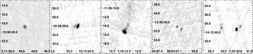
Figure 6: Sample images of our five source classes. The images are drawn from our new VLA observations and show, from left to right, a log intensity grayscale map of sources with decreasing compactness: “P”, “S”, “L”, “D”, and “C.”

Table 7: Morphological classifications for VLA observations.

Morphological class		Fraction	$\langle\alpha_{\mathrm{low}/8.4}\rangle$
“N”	No detection	6.0%	N/A
“P”	Point source	84.3%	$-0.177\pm 0.008$
“S”	Short jet	5.1%	$-0.444\pm 0.028$
“L”	Long jet	3.6%	$-0.428\pm 0.035$
“D”	Double	0.6%	$-0.691\pm 0.068$
“C”	Complex	0.4%	$-0.444\pm 0.155$

6 Conclusions

We have assembled a large and nearly uniform catalog of interferometric observations of bright flat-spectrum radio sources. This list should be particularly valuable for statistical comparison with other all-sky surveys. We should remember that the GB6 parent catalog of this survey is now some 20 y old. Given that these sources are significantly variable, we would not be surprised if some new bright flat-spectrum sources have appeared in the interim. However, this survey is the most complete list of such objects at present. Since such flat-spectrum sources are argued to dominate the source population at both microwave and GeV energies (Giommi et al., 2006), this catalog will be especially useful for comparison with the forthcoming Planck and GLAST/LAT sky surveys. Planck should have a sensitivity $\geq$30$\times$ that of WMAP for point sources, with a typical positional uncertainty of $5-10\arcmin$, and should detect several thousand sources at $5\sigma$ significance. Similarly, the LAT sky survey of the GLAST mission is expected to detect 1,000$-$10,000 blazars (Chiang & Mukherjee, 1998). Sowards-Emmerd et al. (2005) have shown that core flux density and spectral index can be used to select likely counterparts of $\gamma$-ray blazars, so this survey should be ideal for application to the GLAST/LAT survey detections. Indeed, we have selected a $\sim$15% subset of this survey with the greatest similarity (in terms of flux density, spectral index, and X-ray emission) to the EGRET blazars and are completing optical identifications of this sample (CGRaBS, the Candidate Gamma-Ray Blazar Survey; Healey et al. 2007).

These interferometric observations provide the sub-arcsecond positions needed to make reliable optical associations to faint ($R\sim 23$) magnitudes. For the VLA observations, we also have good sub-arcsecond scale structure for many sources, which allows some basic morphological classification. As expected for such a flat-spectrum sample, most sources are unresolved point sources (“P”). These compact sources provide a convenient, relatively bright set of potential atmospheric phase fluctuation calibrators for, e.g., ALMA, CARMA, MERLIN, and the VLBA. In the $-40^{\circ}<\delta<75^{\circ}$ region, our “P” sources with $S_{8.4\>\mathrm{GHz}}\geq 50$ mJy provide $0.217/\sq^{\circ}$ potential calibrators. We also have a significant population of short (“S,” $\leq$$1\arcsec$) jet emission sources, while the number of more complex sources is small. The ATCA data also show a handful of “D”-, “L”-, and “C”-class sources, but most are de facto “P.” The areal density of potential compact sources in this region is $0.225/{\rm deg^{2}}$, but of course these are only known to be compact at the $\sim$$2\arcsec$ scale. In general, we expect the most compact sources to have the highest (flattest) spectral indices and the largest variability. A crude measure of the component compactness or core domination can be inferred from $S_{\mathrm{max}}/\Sigma S$, where $S_{\mathrm{max}}$ is the flux density of the brightest component and $\Sigma S$ is the sum of the flux densities of all components. In the left panel of Figure 7, we see that $\alpha$ does indeed increase as one moves from “D” to “P” sources. However, the few complex “C” sources have a large range of $\alpha$ values and a larger uncertainty in the mean.

In the right panel, the trend is also clear, but we see that some complex, double, and extended jet sources lie above the main distribution, to the upper left. Interestingly, about 1/2 of known lenses (Browne et al., 2003; Winn et al., 2002) in CRATES lie in this region of extended structure but overall flat spectrum, so we infer that in some cases flat-spectrum “C” sources are created by multiple imaging of compact cores.

Figure 7: Spectral index $\alpha_{\mathrm{low/8.4}}$ as a function of morphological class.
Left: the median $\alpha$ value for each class plotted with the error bar for its uncertainty and the 68% range of spectral indices in the class (dashed error bars). There is a general trend toward flatter spectra as the sources are increasingly core-dominated.
Right: spectral index as a function of compactness (core domination). Point sources (“P”) and short jets (“S”) are shown as dots, long jets (“L”) and extended doubles (“D”) as triangles, and complex (“C”) sources as circles. Unresolved (“P”) sources are shown in the band at right. The trend toward increasing $\alpha$ at increased compactness is clear. The handful of non-compact, flat-spectrum sources has a large fraction of known gravitational lenses.

We have also probed the variability of our sample, characterizing the source variability as that of its brightest component: $\mathrm{RMS}(S_{i})/\langle S_{i}\rangle$. Our sampling of this variability is highly non-uniform, with epoch separations spanning $\sim 1-10$ y. The mean variability of unresolved cores with multi-epoch observations was 14%. While the mean variability of the short jets was 12%, the number of multi-epoch measurements was too small to discern clear differences. Interestingly, the few doubles and complex sources with multi-epoch data showed rather high variability of 20-30%. This may, however, be a selection effect as a large number of gravitational lenses and lens candidates are in these classes; these may have attracted more follow-up observations in the extended lens surveys and are more likely to be measurably variable.

The primary purpose of the CLASS survey was to discover gravitational lenses, and 22 were found in the $\sim$12,000 sources observed (Browne et al., 2003). We have included $\sim$4800 sources from the CLASS set and have independently recognized several gravitational lenses in our map inspections, especially among the “C” sources. Similarly, gravitational lens searches were the main focus of most of the CRATES-Va projects, and at least four gravitational lenses have been identified from a sample of 4000 sources observed in these programs (Winn et al., 2002). Fifteen published lenses from these two survey sets are in the CRATES sample. As it happens, only $\sim$300 sources north of $\delta=-40^{\circ}$ were uniquely observed in our new VLA observations CRATES-V1, -V2, -V3. Thus, scaling from the CLASS discovery rate ($\sim$1 lens / 550 flat-spectrum sources), we would not expect any new lens discoveries in this data set. However, the CRATES-Va reprocessing and the multi-epoch comparison of some sources have produced improved maps and component measurements. During our spectral analysis and classification exercise, we have flagged a number of lens candidates for which we will be pursuing follow-up observations. We have collected initial maps of a larger fraction of the Far Southern sources, but since the resolution ($\sim 1\arcsec$ for the maximum 6 km baseline) is not really high enough for lens searches, it is not surprising that only a few show sufficient resolved structure to be worthy of further study.

In summary, we have assembled a large, targeted cm-wavelength survey of compact flat-spectrum sources, covering the full extra-Galactic sky. While many of the observations used in this catalog were mined from the VLA and ATCA archives, over 40% of the positions and flux densities are published here for the first time. We have attempted to make the sensitivity, flux density scale, and astrometric quality as uniform as possible. We expect that upcoming all-sky surveys, especially the GLAST/LAT and Planck surveys, will find this catalog an excellent list for making statistical association with flat-spectrum counterparts and for large-sample studies of their multiwavelength properties. We expect that blazar studies will particularly benefit from this large, uniform survey. We are now focusing on the best candidates for high-energy blazar emitters and collecting multiwavelength associations and spectral IDs. While there are other important blazar classification efforts underway (e.g., Massaro et al. 2005), we hope that the extent and uniformity of the CRATES sample will make statistical studies with these objects particularly powerful.

References

- Becker at al. (1995) Becker, R. H. et al. 1995, ApJ, 450, 559.
- Bock et al. (1999) Bock, D. C.-J. et al. 1999, AJ, 117, 1578.
- Browne et al. (2003) Browne, I. W. A. et al. 2003, MNRAS, 341, 13.
- Chiang & Mukherjee (1998) Chiang, J. & Mukherjee, R., 1998, ApJ 496, 752.
- Condon et al. (1998) Condon, J. J. et al. 1998, AJ, 115, 1693.
- Douglas et al. (1996) Douglas, J. N. et al. 1996, AJ, 111, 1945.
- Giommi et al. (2006) Giommi, P. et al. 2006, A&A, 445, 843.
- Gregory et al. (1996) Gregory, P. C. et al. 1996, ApJS, 103, 427.
- Griffith & Wright (1993) Griffith, M. R. & Wright, A. E. 1993, AJ, 105, 1666.
- Hartman et al. (1999) Hartman, R. C. et al. 1999, ApJS, 123, 79.
- Healey et al. (2007) Healey, S. E. et al. 2007, ApJ, in prep.
- Hinshaw et al. (2006) Hinshaw, G. et al. 2006, submitted.
- Kühr et al. (1981) Kühr, H. et al. 1981, AJ, 86, 854.
- Massaro et al. (2005) Massaro, E., Sclavi, S., Giommi, P., Perri, M., & Piranomonte, S. 2005, Aracne Editrice, A02-26S.
- Mattox et al. (2001) Mattox, J. R. et al. 2001, ApJS, 135, 155.
- Mauch et al. (2003) Mauch, T. et al. 2003, MNRAS, 342, 1117.
- Myers et al. (2003) Myers, S. T. et al. 2003, MNRAS, 341, 1.
- Rengelink et al. (1997) Rengelink, R. B. et al. 1997, A&AS, 124, 259.
- Ricci et al. (2004) Ricci, R. et al. 2004, MNRAS, 354, 305.
- Sadler et al. (2006) Sadler, E. M. et al. 2006, MNRAS, 371, 898.
- Sowards-Emmerd et al. (2004) Sowards-Emmerd, D. et al. 2004, ApJ, 609, 564.
- Sowards-Emmerd et al. (2005) Sowards-Emmerd, D. et al. 2005, ApJ, 626, 95.
- Winn et al. (2000) Winn, J. N. et al. 2000, AJ, 120, 2868.
- Winn et al. (2002) Winn, J. N. et al. 2002, ApJ, 564, 143.
-
Wright et al. (1997)
Wright, A. E. et al. 1997, unpublished catalog available from
http://www.parkes.atnf.csiro.au/research/surveys/pmn/casouth.pdf