Photometric observations of Rosetta target asteroid 2867 Steins

Asteroid 2867 Steins is one of two flyby targets of ESA’s International Rosetta Mission, launched in March, 2004. We obtained CCD observations of Steins on April 14-16, 2004 at Table Mountain Observatory, California, in order to characterize the asteroid physically, information that is crucial for planning the Steins flyby. This study includes the first detailed analysis of the physical properties of Steins from time-series $R$-filter data along with $V$- and $I$-filter photometric measurements. We found a mean $R$-filter absolute magnitude of $12.60$ $\pm$ $0.02$ (for G=0.15), corresponding to a mean radius of $3.57$ $\pm$ $0.03$ km assuming an S-type reflectance of 0.20, or $2.24$ $\pm$ $0.02$ km assuming an E-type reflectance of 0.40 (and G=0.40). The observed brightness range of $0.29$ $\pm$ $0.04$ magnitudes suggests a lower limit on the axial ratio, $a/b$, of 1.30. We determined a synodic rotation period of $6.048$ $\pm$ $0.007$ hours, assuming a double-peaked lightcurve. We fitted the available $R$-filter photometry over the phase angle range of 11.08–17.07 degrees and found best-fit phase function parameters of G=$0.46^{+0.32}_{-0.20}$, and H=$12.92^{+0.22}_{-0.17}$. Derived colour indices for the asteroid are ($V-R$) = $0.58$ $\pm$ $0.03$, and ($R-I$) = $0.44$ $\pm$ $0.03$. These values are consistent with, though slightly redder than Hicks et al. (IAUC 8315). Barucci et al. (barucci (2005)) identified Steins as an E-type based on visual and near-infrared spectra, but if that is correct, then it is an unusually red E-type asteroid.

1 Introduction

Asteroid 2867 Steins is one of two flyby targets of the European Space Agency’s International Rosetta Mission, launched on March 2, 2004. Rosetta will rendezvous with periodic comet 67P/Churyumov-Gerasimenko in 2014. En route to the comet, Rosetta will fly by two main belt asteroids, 2867 Steins on September 5, 2008 and 21 Lutetia on July 10, 2010. As the targets were changed due to the Rosetta launch delay from 2003 to 2004, the new target comet and flyby asteroids have little observational data available (with the exception of Lutetia). Thus, new studies like this one are needed to build up a detailed picture of the physical and surface characteristics of asteroid Steins.

Asteroid 2867 Steins is located in the inner main belt at a semi-major axis of 2.363 AU. Orbital elements for the asteroid are given in Table 1. Its absolute $R$-band magnitude of 12.67 from unpublished measurements (Hicks et al. IAUC 8315) corresponds to a mean diameter of 6.9 km if it is a typical S-type with albedo = 0.20 or 4.9 km for a E-type object with albedo = 0.40. Hicks et al. found $BVRI$ colours consistent with an S-type taxonomic classification, though they could not rule out a D-type object. However, Barucci et al. (barucci (2005)) classified 2867 Steins as an E-type asteroid based on visual and near-infrared spectra taken in January and May, 2004. E-type asteroids are similar to enstatite achondrite meteorites, one of the more thermally processed classes.

Polarization curves at wavelengths of $R$ and $V$ passbands were obtained by Fornasier et al. (fornasier (2006)) from observations with ESO’s VLT telescope, and suggest an albedo of $0.45$ $\pm$ $0.10$. Unfortunately, with this method there is a large scatter in the albedo/polarimetric-slope relation that will inevitably lead to a large uncertainty in the implied albedo. Preliminary analysis of observations of Steins with the Spitzer Space Telescope, combined with visual data, suggest a somewhat lower albedo of $0.30-0.40$ (Lamy et al. lamy (2006)).

We observed 2867 Steins in April, 2004 to characterize the asteroid physically. Knowledge of the asteroid’s size, shape, rotation period, and spectral behaviour are crucial in planning the science observations of Rosetta. In addition, lightcurves obtained at multiple apparitions can be used to derive a full three-dimensional shape model and rotation pole orientation, again very important for planning of the Steins flyby. This was done with great success by Kaasalainen et al. (kaasalainen (2003)) for asteroid 25143 Itokawa, target of the Hayabusa sample return mission. Comparison of spacecraft observations with results derived from telescopic observations also provides critical ground truth for remote observing and data analysis techniques.

This paper is organized as follows. Section 2 describes the observational configuration and strategy employed for this programme. Section 3 describes the analysis techniques that were applied to the data, and the results on the bulk physical and surface properties are also presented. A summary of the results and main conclusions is given in the final section.

2 Observations of 2867 Steins

Asteroid 2867 Steins was observed with the 0.6 meter, Ritchey-Chretien telescope at the Table Mountain Observatory (TMO), near Wrightwood, California on April 14-16, 2004 (UT). The observing geometry of the asteroid on each date is listed in Table 2. Images were obtained with the facility CCD camera, using a Photometrics $1024\times 1024$ pixel thinned and back-illuminated CCD, mounted at the Cassegrain focus of the f/16 telescope. The pixel scale was 0.52^′′/pixel and the total field-of-view was $8.9^{\prime}\times 8.9^{\prime}$. For all images the telescope was tracked at the asteroid’s predicted rate of motion based on an ephemeris from JPL’s Horizons system (Giorgini and Yeomans giorgini (1999)).

The asteroid was located slightly past opposition and at a northern declination of +20^∘, allowing observations below two air masses for about six hours per night. Observations were conducted using the Johnson/Kron-Cousins $VRI$-filter set. A total of 38 $R$-filter images of the asteroid field were obtained on night 1, 36 on night 2, and 39 on night 3. Typical exposure times were 360-600 seconds. Additionally, on night 2, one $V$-filter and one $I$-filter image each were obtained as part of an R-V-R-I-R sequence. Each night’s observations included twilight sky frames in the $R$-filter (plus the $V$ and $I$ filters on night 2), bias (zero exposure) frames, and Landolt fields (Landolt landolt (1992)) imaged over a range of air masses. Observing conditions on nights 1 and 3 were photometric while night 2 suffered from some high cirrus. Because of this, calibration frames of the Steins star fields for night 2 were obtained on a later run at TMO under photometric conditions. The Landolt fields used were PG1047+003, PG1323-086, and PG1528+062 (Landolt landolt (1992)).

3 Data reduction and analysis

All images were bias-subtracted and flat-fielded, and other instrumental artifacts, such as cosmic rays and bad rows/columns were removed in the standard manner. Standard aperture photometry was applied to the images using an aperture $\sim$3 times the maximum measured seeing each night. Image processing was performed using the Image Reduction and Analysis Facility (IRAF) (Tody tody86 (1986); tody93 (1993)).

3.1 Shape, size, and surface colour

A relative asteroid lightcurve was extracted from the imaging for each night by comparing the asteroid’s $R$-filter brightness with that of non-varying field stars in the same images. The observed rotational lightcurve was asymmetric, and the observed full brightness range was $0.29$ $\pm$ $0.04$ magnitudes. This implies an axial ratio, $a/b$, of $\geq$ $1.30$ $\pm$ $0.04$, using $a/b\geq 10^{0.4\Delta m}$, where $a$ and $b$ are the semi-axes of the asteroid and $\Delta m$ is the range of observed magnitudes. This simple model assumes a bi-axial ellipsoid shape and uniform surface albedo, and ignores phase effects. Zappalà et al. (zappala (1990)) analysed the relationship between lightcurve amplitudes and phase angles for a subset of known asteroid classes. They showed that the lightcurve amplitude increases with phase angle, and that the degree of change is dependent on the taxonomic class of the asteriod. More specifically,

$$\Delta m(0^{\circ})=\frac{\Delta m(\alpha)}{1+\kappa\alpha}$$ (1)

where $\Delta m(0^{\circ})$ and $\Delta m(\alpha)$ are the lightcurve amplitudes at $0^{\circ}$ and $\alpha^{\circ}$. The constant $\kappa$ [deg^-1] has values of 0.030, 0.015, 0.014, and 0.013 for S, M, R, and C asteroid taxonomic types, respectively. Taking the $\kappa$ value for S-types and applying equation 1 gives $\Delta m(0^{\circ})$ = 0.188 and a corrected axial ratio of 1.19. Unfortunately, no $\kappa$ value is available for E-type asteroids therefore we use the S-type value based on the very red colour indices of 2867 Steins (see below).

The calibrated apparent magnitudes from our Table Mountain run on April 14-16, 2005 are listed in Table 3 (see the online version of this paper). The mean calibrated $R$-filter apparent magnitude, or the apparent magnitude at lightcurve mid-point is $16.80$ $\pm$ $0.02$. If we assume an S-type phase-slope parameter G of 0.15 in the standard HG system of Bowell et al (bowell (1989)), as used by Hicks et al. (IAUC 8315), we obtain a mean absolute $R$-filter magnitude of $12.60$ $\pm$ $0.02$. This is brighter by 0.07 magnitudes than the Hicks et al. measurement, but consistent at the 2$\sigma$ level. Alternatively, if we assume a typical G value of 0.40 for an E-type asteroid, we obtain a mean absolute $R$-filter magnitude of $12.86$ $\pm$ $0.02$.

Assuming a typical S-type albedo of 0.20 (and S-type G value), our mean apparent $R$-filter magnitude implies a mean effective radius of $3.57$ $\pm$ $0.03$ km or semi-axes of $3.42$ $\pm$ $0.03$ and $4.06$ $\pm$ $0.03$ km if the phase-angle-corrected lightcurve magnitude range is considered. Assuming a typical E-type albedo of 0.40 (and E-type G value of 0.40), our mean apparent magnitude implies a smaller mean effective radius of $2.24$ $\pm$ $0.02$ km with semi-axes of $2.14$ $\pm$ $0.02$ and $2.54$ $\pm$ $0.02$ km, again using the corrected axial ratio of 1.19. We use the size-magnitude relationship of Russell (russell (1916)).

To remove the confounding effects on the derived colour indices due to possible projected area variation with rotation, we compared the $V$ and $I$ apparent magnitudes with interpolated $R$-filter measurements from Table 3 (included in the online version of this paper). We took the average of the two bracketing $R$-filter data points for each of the $V$ and $I$ measurements, and measured the difference to get the ($V-R$) and ($R-I$) colour indices. Our quoted ($V-I$) is the summation of these two colour indices and not the difference between the actual $V$ and $I$ apparent magnitudes.

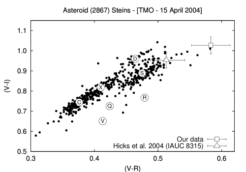
Figure 1: Comparison of our colours with Hicks et al. (IAUC 8315), and ECAS data from Zellner et al. (zellner (1985)). The positions of the main Tholen classes are marked (Tholen tholen (1984)). Our colour data is consistent with Hicks et al. at the 1.2$\sigma$ level, but are much redder than typical E-types (i.e. X-type) bodies. Barucci et al. (barucci (2005)) assign an E-type classification to Steins due to the presence of a 0.49 $\mu$m absorption feature in their spectrum.

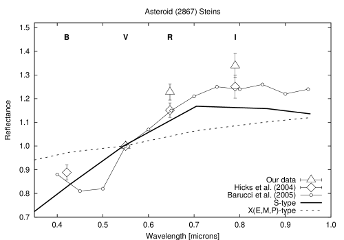
Figure 2: Here we compare the available visual broad-band photometry and spectroscopy for Steins. We include the reflectance spectrum from Barucci et al. (barucci (2005)), which has been sampled at 0.05 $\mu$m intervals, and normalized at 0.55 $\mu$m. The broadband colours have been converted to reflectances and normalized at 0.55 $\mu$m (i.e. at $V$-filter wavelengths). Our $VRI$ data is included, along with $BVRI$ photometry from Hicks et al. (IAUC 8315). One can see that the Barucci et al. spectrum agrees very well with the Hicks et al. data set. Our data is slightly redder than the rest, but still in agreement within the photometry uncertainties and the noise level of the spectrum. We have also included mean reflectance spectra for the Tholen X- and S-types. The photometry and spectroscopy all show that the spectrum is much redder than a typical E-type, though there are a few E-type outliers that approach the redness of the Steins spectrum.

The interpolated colour indices are given in Table 4, along with the corresponding $R$ magnitude, and the values found by Hicks et al. (IAUC 8315). Our values are somewhat redder than Hicks et al. but consistent at the $1.2\sigma$ level. In Figure 1 we compare these colours with similar colour indices for other asteroids, derived from ECAS data (zellner (1985)) using the transformation method discussed in Dandy et al. (dandy (2003)). Based on our colours we find that the visible colours for this asteroid are much redder than typical E-type asteroids. As noted above, Barucci et al. (barucci (2005)) report an E-type classification for Steins based on visual and near-infrared spectra, in particular the presence of a 0.49 $\mu$m absorption band. New preliminary colour data from Weissman et al. (personal communication), based on observations from Cerro Tololo in August 2005, give results similar to both Hicks et al. and our results presented here. Thus, all available visible colours of 2867 Steins agree. We compare our results with those of Hicks et al. (hicks (2004)) and the Barucci et al. (barucci (2005)) spectrum in Figure 2. All three data sets of Steins agree on its strong red colour. If Steins is an E-type asteroid, then it is unusually red.

The differences in our colours and those by Hicks et al. (hicks (2004)) may be indicative of surface inhomogeneities, resulting in areas of differing spectral slopes, perhaps from shifting of surface regolith. Such a mechanism could explain the fascinating surface characteristics of asteroid Itokawa as observed by the Hayabusa asteroid-rendezvous spacecraft (Fujiwara et al. fujiwara (2006); Abe et al. abe (2006)). This issue could be addressed by obtaining rotationally resolved spectra of 2867 Steins. Otherwise, it must await the examination of Steins by the Rosetta spacecraft in 2008.

3.2 Photometric phase function

We used the available $R$-filter photometry to assess the phase-angle variation of the asteroid’s brightness. Our data are combined with the Hicks et al. data (IAUC 8315) to perform a fit of the photometric phase function in terms of the HG formalism. The Hicks et al. data and our data were taken when Steins was at average phase angles of 11.07 and 17.07 degrees, respectively. For the fit we use Hicks et al’s. mean apparent magnitude of $16.53$ $\pm$ $0.02$ and convert to ‘reduced’ magnitude R(1,1,$\alpha$), i.e. the apparent magnitude has been scaled to unit heliocentric and geocentric distances. The reduced magnitude is $13.36$ $\pm$ $0.02$. We do the same for our mean $R$-filter apparent magnitude of $16.80$ $\pm$ $0.02$, and the resulting reduced magnitude is $13.51$ $\pm$ $0.02$.

The best fit photometric values are G=0.46 and H=12.92. When the 1$\sigma$ photometric uncertainties in the mean apparent magnitudes are considered we find that G values of 0.26 and 0.78 fit the data just as well. The corresponding H values are 12.75 and 13.14, respectively, and the fits are shown graphically in Figure 3. The accepted phase function parameters and 1$\sigma$ uncertainties are therefore G=$0.46^{+0.32}_{-0.20}$, and H=$12.92^{+0.22}_{-0.17}$. Although there is no phase coverage within the opposition-surge region at small phase angles we still prefer to fit for G rather than simply applying a linear phase law that is inappropriate for asteroidal bodies.

A shallow slope parameter of G=0.46 is more associated with E-type asteroids than S-type. Because of the large error bar we cannot put too much weight on our derived slope parameter as a means of distinguishing whether or not the asteroid is either type. At the very least, this would require refinement of our phase-slope measurement through opposition surge coverage along with observations at large phase angles. Nevertheless, this result will aid in better assessment of the brightness of Steins for future observational planning, which needs to take place at a wide range of observational geometries, allowing for the full 3-D shape and orientational modelling to take place. Taken together, these data will also allow a full Hapke-type analysis to be performed (e.g. Lederer et al. lederer (2005)), providing detailed information on Steins’ surface regolith.

For completeness, we compute the corresponding effective radius using this fitted H value and for assumed typical geometric albedos of both S-type and E-type asteroids. For a typical S-type albedo of 0.20, the absolute magnitude corresponds to an effective radius of $3.08^{+0.25}_{-0.30}$ km, and for an E-type albedo of 0.40, the absolute magnitude corresponds to an effective radius of $2.18^{+0.18}_{-0.21}$ km.

3.3 Rotational properties

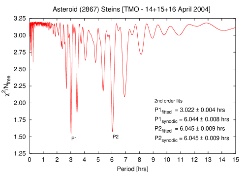
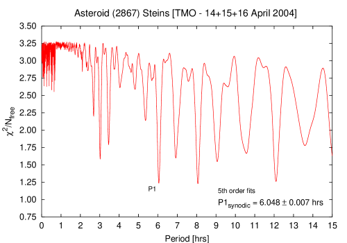
Figure 4: Upper panel: Resulting periodogram from 2nd order Fourier fits to the relative magnitudes. We find a best synodic period of $6.045$ $\pm$ $0.009$ hours. Note the ‘dual’ structure of the periodogram which is expected for an asteroid lightcurve with near sinusoidal shape. Lower panel: Periodogram for a 5th order Fourier series fit to our $R$-filter time series data. These higher order fits were performed in order to improve the accuracy of the period. We find a best-fit synodic rotation period of $6.048$ $\pm$ $0.007$ hours. The feature near 8 hours is not physically realistic as it produces a triple-peaked lightcurve. The other prominent feature near 12 hours is a harmonic of 6.048.

We applied the method of Harris et al. (harris (1989)) to determine the rotation period. This method involves fitting an nth-order Fourier series to the relative magnitudes, which is then repeated for a wide range of periods until the fit residuals are minimized. The chosen range of periods depends on initial inspection of the lightcurves. When fitting model lightcurves to the data, we start with low order fits to get a feel for where the prominent periodicities reside. We then increase the order to refine the dominant periodicity and its associated uncertainty, and also the quality of the fit. We stop increasing the order once the quality of the fit no longer improves. It was clear from our initial inspection of the data that the asteroid was rotating in $\sim$6 hours, assuming a double-peaked lightcurve. We created a periodogram over the reasonable range of 0–15 hours, which is shown in the upper panel of Figure 4. This periodogram results from 2nd order fits and shows the location of two dominant periodicities. As we know the object has a full rotation period of just over 6 hours (assuming a double-peaked lightcurve), we adopt the feature at 6.045 hours as the measured synodic period. The other prominent minima at 3.022 hours is simply the result of folding the lightcurve at half this frequency resulting in low fit residuals, which is expected for an asteroid lightcurve with near sinusoidal shape. If the lightcurve had a more asymmetric shape, then the periodogram feature around 3.022 hours would be much less prominent.

Our final fit, using a 5th order polynomial to refine the period estimate above, is shown in the lower panel of Figure 4. Prominent minima are seen at approximately 6, 8, and 12 hours. The best-fit synodic period is $6.048$ $\pm$ $0.007$ hours. The feature near 8 hours is not physically realistic as it produces a triple peaked lightcurve. The other prominent feature near 12 hours is just a harmonic of 6.048.

In Figure 5, we plot the relative magnitudes vs rotational phase. The points are folded to the best-fit synodic period of 6.048 hours, and the relative magnitudes for each night have been scaled according to their nightly averages and then centered around zero, so that small geometry changes are accounted for in the folding of the data points. The double-peaked asymmetric lightcurve covering one full rotation is clearly visible each night. Our derived period agrees well with the previous value obtained by Hicks et al. (IAUC 8315), who found a period of $6.06$ $\pm$ $0.05$ hours.

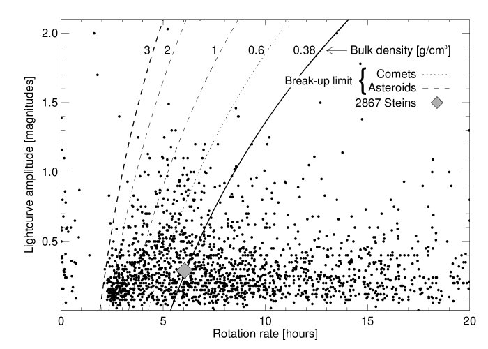
Figure 6: Comparison of our Steins rotational lightcurve parameters with other asteroidal bodies. The curves are lines of constant bulk density for a simple centrifugal break-up model (see text). The rubble-pile breakup limit is shown for the asteroid population at a density of 3 g/cm³. The equivalent break-up limit for cometary nuclei at 0.6 g/cm³ is also marked. The location of Steins on this chart indicates that this asteroid is very typical of asteroidal bodies. From this model we measure a bulk density lower limit for Steins of 0.38 g/cm³.

In Figure 6 we compare our Steins rotational lightcurve parameters with other asteroidal bodies. The overplotted curves are lines of constant bulk density for a simple centrifugal break-up model, and for various density values. For a strengthless prolate ellipsoidal body, the critical rotation period $P_{critical}$ - beyond which a body will be broken apart by centrifugal forces exceeding self gravity - can be approximated by

$$P_{critical}\approx\frac{3.3}{\sqrt{\rho}}\sqrt{\frac{a}{b}}$$ (2)

where $P_{critical}$ is in units of hours, $\rho$ [g/cm³] is the bulk density of the body, and $a/b$ is the axial ratio derived from the lightcurve amplitude as described in section 3.1 (Pravec & Harris pravec_harris (2000)). $P_{critical}$ and $\rho$ are derived directly from the lightcurve, although the latter is only a lower limit as the rotation axis orientation is unknown and the derived axial ratio is the projected value. Also, there is no requirement that the asteroid be rotating at its critical period. Therefore one can only obtain a lower limit to the bulk density from the lightcurve parameters.

The rubble-pile breakup limit is shown for the asteroid population at a density of 3 g/cm³. The only asteroids that are able to spin faster than the $\sim$2 hour spin rate are the so-called monolithic fast rotators. The equivalent break-up limit for cometary nuclei is also marked at 0.6 g/cm³ (Lowry and Weissman lowry (2003)). One can see that Steins is very typical in terms of rotation period and elongation. We applied this simple break-up model to Steins to place a bulk density lower limit of 0.38 g/cm³. Strictly speaking, the full magnitude range is not yet known, which could affect this density lower limit determination.

4 Discussion and Summary

We have analyzed results from photometric observations of the Rosetta mission flyby target asteroid 2867 Steins, obtained on April 14-16, 2004 (UT) at the Table Mountain Observatory, California. These data, when combined with future data at different observing geometries, will be critical for developing a detailed 3-D shape and orientation model (crucial for Rosetta’s science and operations planning), as well as allowing surface properties to be investigated in detail prior to the flyby in September 2008. Our main conclusions are as follows:

1. We measured a mean apparent $R$-filter magnitude of $16.80$ $\pm$ $0.02$. If we assume a phase-slope parameter G of 0.15, as used by Hicks et al. (IAUC 8315), we obtain a mean absolute $R$-filter magnitude of $12.60$ $\pm$ $0.02$. This is slightly brighter than the Hicks et al. measurement but consistent at the 2$\sigma$ level. If we assume a typical E-type-asteroid G value of 0.40 (the type assigned to Steins by Barucci et al. barucci (2005)) we obtain a mean absolute $R$-filter magnitude of $12.86$ $\pm$ $0.02$.

2. The observed rotational lightcurve was asymmetric, and the observed full brightness range was $0.29$ $\pm$ $0.04$ magnitudes. This implies an axial ratio, $a/b$, of $\geq 1.30$ $\pm$ $0.04$.

3. We fitted a 5th order Fourier series to the time-series relative magnitudes and found a best-fit synodic rotation period of $6.048$ $\pm$ $0.007$ hours, in good agreement with other observers. The rotation rate and shape of Steins is very typical for asteroidal bodies. Using a centrifugal break-up model we determined a bulk density lower limit of 0.38 g/cm³.

4. Assuming a typical S-type albedo of 0.20 (and G=0.15), our mean apparent $R$-band magnitude implies a mean effective radius of $3.57$ $\pm$ $0.03$ km or semi-axes of $3.42$ $\pm$ $0.03$ and $4.06$ $\pm$ $0.03$ km if the full phase-angle-corrected magnitude range is considered. Assuming a typical E-type albedo of 0.40 (and G=0.40), we obtain a smaller mean effective radius of $2.24$ $\pm$ $0.02$ km or semi-axes of $2.14$ $\pm$ $0.02$ and $2.54$ $\pm$ $0.02$ km.

5. We use the available $R$-filter photometry for a preliminary assessment of the phase-angle variation of the asteroid’s brightness. We combined our mean apparent magnitudes with the Hicks et al. data (IAUC 8315) to perform a fit of the photometric phase function in terms of the HG formalism. The best fit phase function parameters and associated 1$\sigma$ uncertainties are G=$0.46^{+0.32}_{-0.20}$, and H=$12.92^{+0.22}_{-0.17}$. Opposition-surge coverage would be useful along with observations at large phase angles in order to refine this measurement.

6. Our measured colour indices are: ($V-R$) = $0.58$ $\pm$ $0.03$, ($R-I$) = $0.44$ $\pm$ $0.03$, and thus ($V-I$) = $1.03$ $\pm$ $0.04$. These values agree well with Hicks et al. (IAUC 8315) but suggest that if Steins is an E-type asteroid as suggested by Barucci et al. (barucci (2005)), then it is an unusually red E-type object.

Table 1: Orbital elements: 2867 Steins

Element	Valuea
semimajor axis	2.3633 AU
eccentricity	0.145478
inclination	9.9456 degrees
argument of perihelion	250.4844 degrees
longitude of ascending node	55.5399 degrees
time of perihelion	2001 Nov. 04.21279

• Epoch: 2005-Jan-30.

Table 2: Observing geometry (at 4 hr UT)

Date	r (AU)	$\Delta$ (AU)	Phase angle (deg.)
14 April 2004	2.5601	1.7731	16.78
15 April 2004	2.5588	1.7809	17.07
16 April 2004	2.5576	1.7890	17.35

Table 3: Apparent $R$-filter magnitudes

Date†	$m_{R}$ $\pm$ $\sigma$	Date†	$m_{R}$ $\pm$ $\sigma$	Date†	$m_{R}$ $\pm$ $\sigma$
09.62304	16.763 $\pm$ 0.032	10.62904	16.811 $\pm$ 0.020	11.62060	16.808 $\pm$ 0.024
09.62857	16.771 $\pm$ 0.030	10.63420	16.771 $\pm$ 0.018	11.62598	16.790 $\pm$ 0.023
09.63371	16.787 $\pm$ 0.030	10.63939	16.801 $\pm$ 0.018	11.63113	16.761 $\pm$ 0.018
09.63990	16.858 $\pm$ 0.028	10.65213	16.901 $\pm$ 0.019	11.63612	16.761 $\pm$ 0.018
09.64901	16.876 $\pm$ 0.028	10.65789	16.891 $\pm$ 0.018	11.64205	16.758 $\pm$ 0.019
09.65426	16.875 $\pm$ 0.028	10.66877	16.941 $\pm$ 0.018	11.64699	16.796 $\pm$ 0.019
09.68235	16.731 $\pm$ 0.027	10.67967	16.881 $\pm$ 0.019	11.65202	16.847 $\pm$ 0.018
09.68752	16.710 $\pm$ 0.029	10.74053	16.741 $\pm$ 0.018	11.65723	16.892 $\pm$ 0.018
09.69274	16.698 $\pm$ 0.029	10.74587	16.751 $\pm$ 0.018	11.66232	16.926 $\pm$ 0.017
09.69778	16.708 $\pm$ 0.029	10.75133	16.761 $\pm$ 0.018	11.66766	16.974 $\pm$ 0.018
09.70309	16.722 $\pm$ 0.030	10.75642	16.781 $\pm$ 0.018	11.67288	16.993 $\pm$ 0.018
09.70796	16.698 $\pm$ 0.030	10.76155	16.751 $\pm$ 0.018	11.69066	16.874 $\pm$ 0.018
09.71323	16.671 $\pm$ 0.029	10.76674	16.791 $\pm$ 0.018	11.69583	16.858 $\pm$ 0.017
09.71812	16.681 $\pm$ 0.029	10.77238	16.821 $\pm$ 0.019	11.70094	16.772 $\pm$ 0.018
09.72344	16.652 $\pm$ 0.030	10.77748	16.811 $\pm$ 0.018	11.70624	16.772 $\pm$ 0.017
09.72992	16.671 $\pm$ 0.028	10.78270	16.841 $\pm$ 0.019	11.71160	16.753 $\pm$ 0.017
09.73527	16.706 $\pm$ 0.029	10.78789	16.861 $\pm$ 0.019	11.71813	16.755 $\pm$ 0.017
09.75697	16.803 $\pm$ 0.029	10.79314	16.871 $\pm$ 0.019	11.72325	16.751 $\pm$ 0.017
09.76257	16.866 $\pm$ 0.028	10.79837	16.911 $\pm$ 0.019	11.72834	16.737 $\pm$ 0.017
09.76782	16.837 $\pm$ 0.028	10.81798	16.871 $\pm$ 0.020	11.73433	16.758 $\pm$ 0.017
09.77325	16.806 $\pm$ 0.030	10.82328	16.811 $\pm$ 0.019	11.74071	16.776 $\pm$ 0.017
09.77860	16.829 $\pm$ 0.030	10.82836	16.801 $\pm$ 0.018	11.74583	16.767 $\pm$ 0.017
09.78385	16.873 $\pm$ 0.029	10.83333	16.791 $\pm$ 0.019	11.75075	16.753 $\pm$ 0.017
09.78904	16.872 $\pm$ 0.029	10.83837	16.761 $\pm$ 0.019	11.77404	16.860 $\pm$ 0.018
09.79431	16.883 $\pm$ 0.029	10.84334	16.711 $\pm$ 0.018	11.77997	16.889 $\pm$ 0.017
09.79971	16.853 $\pm$ 0.029	10.84851	16.751 $\pm$ 0.019	11.78600	16.840 $\pm$ 0.018
09.80495	16.839 $\pm$ 0.028	10.85445	16.731 $\pm$ 0.019	11.79130	16.841 $\pm$ 0.017
09.81022	16.776 $\pm$ 0.030	10.85966	16.711 $\pm$ 0.020	11.79699	16.846 $\pm$ 0.018
09.83800	16.764 $\pm$ 0.029	10.86466	16.741 $\pm$ 0.020	11.80215	16.869 $\pm$ 0.018
09.84326	16.697 $\pm$ 0.030	10.86982	16.751 $\pm$ 0.019	11.80769	16.845 $\pm$ 0.019
09.84917	16.730 $\pm$ 0.031	10.88739	16.821 $\pm$ 0.020	11.81269	16.890 $\pm$ 0.017
09.85447	16.665 $\pm$ 0.030	10.89260	16.771 $\pm$ 0.021	11.81770	16.849 $\pm$ 0.018
09.85960	16.699 $\pm$ 0.031	10.89749	16.861 $\pm$ 0.019	11.82274	16.854 $\pm$ 0.018
09.86487	16.699 $\pm$ 0.030	10.90264	16.831 $\pm$ 0.020	11.82770	16.824 $\pm$ 0.019
09.87026	16.732 $\pm$ 0.032	10.90776	16.901 $\pm$ 0.021	11.83280	16.807 $\pm$ 0.018
09.87556	16.747 $\pm$ 0.032	10.91278	16.881 $\pm$ 0.020	11.85688	16.766 $\pm$ 0.018
09.88091	16.791 $\pm$ 0.034	–	–	11.88991	16.800 $\pm$ 0.018
09.88637	16.827 $\pm$ 0.037	–	–	11.89593	16.853 $\pm$ 0.020
–	–	–	–	11.90191	16.845 $\pm$ 0.020

$\dagger$ - Light-time corrected mid-exposure-JD minus 2453100

Table 4: $BVRI$ Colours for Asteroid 2867 Steins

Colour	This work	$\overline{R}$†	Hicks et al. (IAUC 8315)
$V-R$	$0.58\pm 0.03$	$16.91\pm 0.02$	$0.51\pm 0.03$
$R-I$	$0.44\pm 0.03$	$16.92\pm 0.02$	$0.44\pm 0.03$
$B-R$	$-$		$1.311\pm 0.03$

$\dagger$ - Corresponding average apparent $R$ magnitude (see text)

Figure 3: We use the available $R$-filter photometry for a preliminary assessment of the phase-angle variation of the asteroid’s brightness in terms of the HG formalism. The best-fit phase function parameters and associated 1$\sigma$ uncertainties are G=$0.46^{+0.32}_{-0.20}$, and H=$12.92^{+0.22}_{-0.17}$. Opposition-surge coverage would be useful along with observations at large phase angles in order to refine this measurement.

Figure 5: The $R$-filter relative magnitudes phased to the best-fit synodic period of 6.048 hours. Data from different nights are distinguished by the various symbol types. The repeatability from night to night is excellent. The full brightness variation was $0.29$ $\pm$ $0.04$ magnitudes.