Determining neutrino properties using future galaxy redshift surveys
Abstract
Current measurements of the large-scale structure of galaxies are able to place an upper limit on the absolute mass scale of neutrinos. An order-of-magnitude improvement in raw sensitivity, together with an insensitivity to systematic effects, is needed to reach the lowest value allowed by particle physics experiments. We consider the prospects of determining both the neutrino mass scale and the number of of massive neutrinos using future redshift surveys, specifically those undertaken with the Square Kilometre Array (SKA), with and without additional constraints from the upcoming Planck CMB experiment. If the sum of the neutrino masses then the imprint of neutrinos on large-scale structure (LSS) should be enough, on its own, to establish the neutrino mass scale and, considered alongside CMB constraints, it will also determine the number of massive neutrinos , and hence the mass hierarchy. If , at the bottom end of the allowed range, then a combination of LSS, CMB and particle physics constraints should be able to determine , and the hierarchy. If is in the specific range , then a combination of LSS, CMB and particle physics experiments should determine , but not or the hierarchy. Once an SKA-like LSS survey is available there are good prospects of obtaining a full understanding of the conventional neutrino sector, and a chance of finding evidence for sterile neutrinos.
keywords:
Cosmology: cosmological parameters – Cosmology: cosmic microwave background – Cosmology: large-scale structure of the universe – surveys – neutrinos1 Introduction
The proof that neutrinos have mass was a major breakthrough in particle physics. This proof came from the observation (e.g. Fukuda et al., 1996) that neutrinos in one weak-flavour state are able to ‘oscillate into’ neutrinos of a different weak-flavour state which, in ‘the vacuum’, is disallowed by quantum mechanics unless neutrinos have mass. The implications of this result are profound not only for particle physics, but also for cosmology. It was the first measured effect that is not included in the Standard Model of particle physics. It also started to set constraints on the absolute mass scale of a particle species which cosmologists have yet to include properly in the energy density budget of the Universe. A recent review of the critical issues is given by Kayser (2005) and another recent review approaching neutrino physics from the theoretical cosmology side is given in Lesgourgues & Pastor (2006).
Throughout this paper we keep with particle physics notation by using natural units in which . We will refer throughout to a ‘fiducial’ cosmology in which the normal cosmological constants take the values: {, , , , } = {0.04, 0.26, 0.72, 1.0, 0.9}. We define as the fraction of critical density contributed by all matter: baryons, CDM and neutrinos. The power spectrum is calculated using the ‘Boltzmann code’ CAMB (Lewis et al., 2000). We reserve the use of the symbol for the absolute mass scale of neutrinos, by which we mean the rest mass of the most massive neutrino (see Fig. 1). Throughout this paper we assume that the Universe is flat and that the ‘dark energy’ is Einstein’s cosmological constant with an equation-of-state parameter .
1.1 Background Particle Physics
Vacuum neutrino oscillations occur if neutrinos are massive because their mass eigenstates are an admixture of the weak-flavour eigenstates familiar from the physics of electroweak interactions. This can be written as
| (1) |
where labels the weak-flavour eigenstates and labels the mass eigenstates. is the mixing matrix that governs the rate of oscillations between different weak-flavour eigenstates. This yields a probability of a given neutrino oscillating from a weak-flavour state to another weak-flavour state of
| (2) |
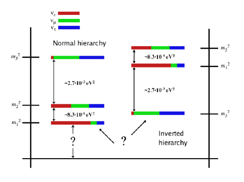
The relationships between the weak-flavour and the mass eigenvectors for neutrinos are illustrated in Fig. 1. The third mass eigenstate is almost perpendicular to the axis of the electron neutrino eigenstate, or to put it in another way the ‘mixing angle’ defined by is small. The experimental evidence for oscillations is summarised by Kayser (2005), but can be very crudely summarised as follows: experiments that probe muon and electron anti-neutrinos originating from cosmic ray showers in the atmosphere can be approximated by a two-neutrino oscillation between muon and tau anti-neutrinos, controlled largely by ; experiments that probe electron anti-neutrinos originating in the sun find strong evidence for a different, but again approximately two-neutrino, oscillation between electron and muon neutrinos, controlled largely by . The current status of quantitative observational results are summarised by Maltoni et al. (2004) (see also Fig. 1).
The mixing matrix can be written in terms of a combination of Euler rotations in an dimensional space, namely
| (3) |
where and are functions of the ‘mixing angles’ . We have assumed that neutrinos behave like Dirac particles – so that each neutrino and its associated anti-neutrino are distinguishable – and we have introduced a phase which allows for Charge-Parity (CP) violations in the sense of small differences between the probability of oscillations between neutrinos and ‘CP-mirror-image’ oscillations between anti-neutrinos.
The transition probability can now be written as
| (4) |
where is the distance between the source and the observer, which is assumed to be a vacuum, and because vacuum oscillations conserve energy, . From Eqn. 4 it is clear why particle physics experiments are mainly sensitive to the differences between the squares of the masses of the mass eigenstates and the mixing angles.
The three main goals of future research into the neutrino sector are as follows: (i) to determine the absolute mass scale for neutrinos; (ii) to determine whether the hierarchy is normal or inverted (see Fig. 1); (iii) to check whether there are so-called sterile neutrinos, particles which interact only via gravity, additional to the three weak-flavour eigenstates. The prospects of rapid progress via further particle physics experiments is limited (Kayser, 2005) and strongly dependent on unknown factors like the true magnitude of , and whether or not the extra diagnostic power available, in principle, from measuring oscillations in the presence of matter can be successfully harnessed.
1.2 Background Cosmology
Neutrinos decoupled from radiation and matter within the first few minutes of the history of the Universe. As this de-coupling occurred before electron-positron annihilation produced an extra source of entropy for the photons, the neutrino temperature has remained at a fraction of the temperature of the CMB given by
| (5) |
Neutrinos remain relativistic until the point at which , which corresponds to a redshift for or for . This means that neutrino free streaming can suppress structure formation on small scales at early times, but the neutrino energy density is dominated by the rest mass at recent times. We assume that there are ‘massive’ neutrinos where for a quasi-degenerate scenario, for an inverted, non-quasi-degenerate scenario and for a normal, non-quasi-degenerate scenario (see Fig. 1). We further assume that neutrinos are Dirac particles so that each neutrino and its associated anti-neutrino are distinguishable. We can then relate the energy density of photons (bosons) to the energy density of neutrinos (fermions). The number density of neutrinos can be related to the number density of photons by , so we can write
| (6) |
Neutrinos behave as a component that transitions from having an equation-of-state , where and are the pressure and energy density respectively, with to as they become non-relativistic. We can evaluate for neutrinos using
| (7) |
where is the degeneracy and is the phase-space distribution function for fermions.
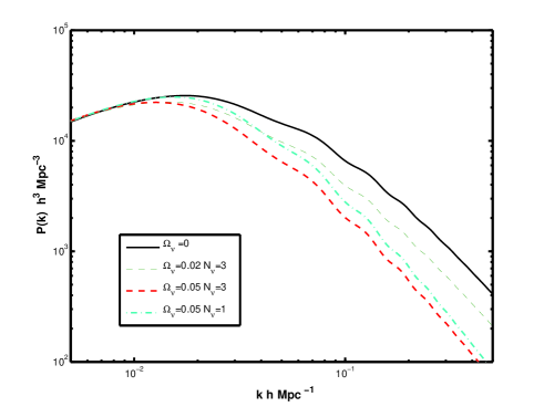
The effect of neutrinos on large-scale structure is illustrated in Fig. 2. The main feature is a strong attenuation of the power spectrum on small scales if there is a significant energy density of neutrinos. This is associated with a preferred length (and ) scale given by the horizon when the neutrinos become non-relativistic which, from Eqn. 1 of (Hu et al., 1998), is
| (8) |
assuming a quasi-degenerate scenario, where is the associated co-moving wavenumber. The damping of the power spectrum at large scales, small , is (Eqn. 2 of Hu et al., 1998) given approximately by
| (9) |
This approximation, although not necessarily accurate on all scales, can be used pedagogically in the following way. This expression assumes which is reasonable because current limits on neutrino energy density (e.g. Elgarøy et al., 2002) firmly exclude anything close to a Hot Dark Matter cosmological model. To measure the effect that neutrinos of a given produce we need to measure more accurately than the fractional shift given by Eqn.9, and we need to ensure that any systematic errors can be neglected.
It is possible to constrain the mass of the neutrino with CMB experiments. However, there are strong parameter degeneracies that prevent this being a very precise tool. It has been shown, nevertheless, that even a neutrino mass as small as 0.05 eV could have a significant effect on the CMB temperature and polarisation power spectrum (Hu et al., 1998; Hannestad, 2003).
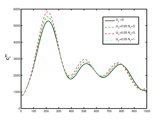
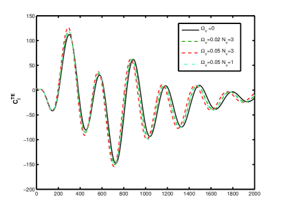
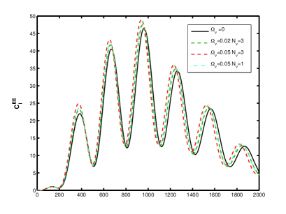
We can see in both Fig.2 and Fig.3 that adding two extra parameters {, } to our fiducial cosmology yields different fluctuations for different values of the parameters. The total energy density in neutrinos is the most important quantity influencing (Eqn.9) but, as explained in the caption to Fig. 2, the suppression of power also depends on . CMB datasets are prone to serious problems with parameter degeneracies: the bound on the neutrino mass are (Ichikawa et al., 2005) claimed to be from WMAP data alone.
2 Methods of making forecasts for future cosmology experiments
Cosmological experiments hold a lot of promise for helping to address the key unknowns in the physics of the neutrino sector. In this section we produce forecasts for the progress possible with upcoming CMB and LSS experiments.
To make these forecasts we will use Markov Chain Monte Carlo (MCMC) methods to probe the dimensional parameter space of cosmological models with different neutrino properties. Such methods (e.g. Bucher et al., 2002) provide a powerful way of forecasting the posterior probability distributions for a given set of cosmological parameters to be probed by a future experiment.
A MCMC is a chain of points drawn and chosen/rejected from a given distribution according to a certain number of rules. Points are chosen from a proposal distribution and either accepted or rejected according to the likelihood attached to both the chosen point and the previous point only (hence a Markov chain). In the simplest algorithms, if the new point has a larger likelihood it is accepted and if the likelihood is lower it is accepted with a probability which equals the ratio of the likelihoods from the old point and the new proposal point. The method is described fully by Lewis & Bridle (2002). If so, the density of points will describe the likelihood function in parameter space.
Given that no real data are available, we proceed in the following way. We first adopt a fiducial cosmology which we will assume is close enough to the truth that it can be used to deliver simulated data. We adopt here a theoretical framework used in Bucher et al. (2002); i.e. we do not produce ensembles of mock datasets but assume that the simulated data is precisely equivalent to the prediction of the fiducial model with an associated, appropriately calculated, error bar. Any single realisation of the data would displace the error ellipse found but would not change its size considerably. The sum over many realisations of the data would produce results which are equivalent to the results obtained by taking the data being equal to the fiducial model, provided, of course, the fiducial model is correct. We use this method for both LSS and CMB forecasts. We then attach theoretical errors to each fiducial data point in line with the errors expected for the future cosmology experiment. Then, we used MCMC chains to map out the dimensional posterior probability distribution function , where
| (10) |
and is the likelihood function (given by in the case of galaxy surveys where is the usual chi squared, i.e. the sum over all simulated data points of the square of the data minus the model divided by the error estimate at that data point) and is the -dimensional prior probability distribution function. We used our fiducial model with the addition of the neutrino parameters and meaning . In the case of simulated LSS surveys more ‘nuisance parameters’ were needed to account for the way in which galaxies trace dark matter: two per redshift shell, making a total of 13 parameters. In the case of the CMB we added the optical depth of reionisation giving a total of 8 parameters. We checked each MCMC chain had converged in two ways: we checked that the means and variances for each of the individual chains (eight MCMC chains were run for each case) were consistent with the other chains and we made a power spectrum amalysis of the chains (Dunkley et al., 2005). Finally, we used the returned MCMC samples to map out the posterior probability distribution.
Our methods are very similar to the Fisher matrix approach (e.g. Hu & Haiman, 2003; Seo & Eisenstein, 2003), in which one also assumes a fiducial cosmology and then calculates the curvature of the posterior probability, assumed to be an dimensional Gaussian, around that point. Both methods assume that the likelihood posterior is a slowly varying function of the fiducial cosmology, but our approach has the advantage of directly mapping out any non-Gaussian features of the posterior probability distribution; in the case of a Fisher analysis any non-Gaussianities of the posterior distribution function may corrupt the error analysis.
2.1 Methods of making forecasts for future LSS experiments
It has been proposed that probing the pattern of matter fluctuations as a function of redshift yields measurements of the Hubble ‘Constant’ and the comoving distance via a characteristic co-moving length scale imprinted on the power spectrum via baryonic oscillations (Blake & Glazebrook, 2003; Hu & Haiman, 2003; Seo & Eisenstein, 2003). This characteristic co-moving length is derivable from known physics, being essentially the size of the sound horizon at the time of last scattering. Given that matter and radiation dominate over dark energy at that period, its length is given by
| (11) |
where introduces a weak dependence of the sound speed of the plasma on and is the scale factor at the redshift of recombination. We can interpret this as a sound speed that is equal to in the case of radiation only and which decreases as a larger fraction of baryons is present.
Therefore we know the precise length of this standard rod for a given cosmology. Furthermore, this distance is dependent on , and weakly on but it is very insensitive to given that this acoustic scale was set up in the early universe when it is thought that dark energy plays a small role.
A related geometric probe of the evolution of the Universe was proposed by Alcock & Paczynski (1979) by assuming that any characteristic length present in the Universe, and which can be seen in both radial and angular directions in the sky, produces a measurement of the product [where is the angular diameter distance] simply because, by isotropy, the length has to be the same in both directions.
This proposed wiggles test (e.g Blake & Glazebrook, 2003; Hu & Haiman, 2003; Seo & Eisenstein, 2003) can therefore simply be considered as a more powerful version of the Alcock-Paczynski (AP) test and should be more useful in constraining dark energy as a geometrical test which is weakly dependent on .
More precisely, the comoving sizes of any object or any feature has a transverse () and parallel projection on the sky which can be used for this kind of test. These comoving features relate to the sizes of the observed angular and redshift distances and respectively via the following relations
| (12) |
Hence, when the true scales are known the measurement of the pattern in or the line of sight and or in the plane perpendicular to the line of sight yield a measurement of and , whereas if the precise value of is not known, it is only the product that can be measured.
To be able to estimate the errors on cosmological parameters we have to know how well we will be able to measure the power spectrum. Under Gaussian conditions, the fractional error on the power spectrum will depend on the total volume of the survey as this will determine the number of Fourier modes that will be sampled by the survey; the associated error is usually called cosmic variance. Furthermore there will be an uncertainty given by the finite number of galaxies. This is commonly termed shot noise. Hence the fractional error on the power spectrum can be written as (Feldman et al., 1994)
| (13) |
where is the power spectrum measured, is the comoving number density of galaxies probed and is the cosine of the angle defined by our line of sight and the line joining pairs of galaxies in 3D space.
If we make a measurement of several effects can change, not only the shape, but also the height of the power spectrum, as a function of redshift. If a wrong cosmology is assumed our estimates of distances and volumes are incorrect. This produces a distortion that is visible in the power spectrum as rings in the (perpendicular, parallel) plane (Hu & Haiman, 2003). Furthermore, at a higher redshift, the growth factor changes the height of the power spectrum. However if a wrong cosmology is assumed, then we have wrong measurements of the cosmological volume in which we made our survey and therefore the height of the power spectrum is measured incorrectly. These distortion effects have been thoroughly described in Ballinger et al. (1996).
If the galaxies are measured in redshift and we do not have any information about their peculiar velocities, we then retrieve a redshift space power spectrum. This will differ from the real space power spectrum in two ways, firstly we obtain more correlations at low because large-scale bulk flows point directly towards matter overdensities due to gravitational pull. Therefore there is an enhancement factor derived in Kaiser (1987), where is the cosine of the angle that the mode which is probed makes with the line of sight, and is the derivative of the natural log of the over-density with respect to the natural log of the scale factor . At large scales, structures appear to be closer to each other in redshift space. On the other hand at small scales, given the circular velocities of satellite and relaxed structures, redshift-space structures appear to be elongated along the line-of-sight. This created the so called finger-of-god effect (Peacock et al., 2001). Here we are interested in the large-scale fluctuations, and we simply ignore the small-scale power , i.e. we include the first effect but not the finger-of-god effect. Note that a complete analysis with real data will need to take both effects into account.
When a galaxy survey is performed it is vital to distinguish between the correlations that we measure in the galaxy distribution and how that distribution relates to the distribution of dark matter. We assume throughout that the non-linear galaxy power spectrum is related to the linear matter power spectrum via . This is motivated by the halo model (e.g. Seljak, 2000; Peacock & Smith, 2000), a galaxy population will most likely not trace matter in an unbiased way and given their discreteness and number density there will be an extra shot noise power attached to the power spectrum.
Therefore in order to estimate cosmological parameters from a galaxy catalogue we first choose a fiducial cosmology which will allow us to change the coordinates from (RA,DEC,z) to spatial coordinates in redshift space. If, presumably by luck, we choose the real cosmology that governs our Universe, then the power spectrum that we will measure as a result of the galaxy autocorrelation function is
| (14) |
However if we chose an incorrect reference cosmology, then we will observe the signal produced from the power spectrum derived from the real cosmological parameters distorted by the incorrect assumption we have made. This results in the following expression, for what measurements of we would retrieve
| (15) |
Hence if an incorrect cosmology is assumed there will be an inconsistency when it comes to compare the power spectrum expected given the assumptions we made about the cosmological parameters. With the power spectrum derived from the data given assumed distances, we will be able to use this inconsistency to probe cosmological parameters. In order to do this, with real data, we simply need to repeat this process for may different cosmological parameters and find which cosmological parameters do not produce any inconsistency by comparing predicted models and measured models assuming the cosmology we are testing.
In both equations 14 and 15 a relationship between () and () depends on cosmology in the following way.
| (16) |
which produce the following relations that we use to convert from a given angle and value in the sky to another distorted angle and value if the incorrect cosmology is chosen
| (17) |
This is a thin shell approximation and strictly speaking should not be used in this analysis. However, we argue that the effect on the power spectrum of using a thin shell approximation, if the shells used are thick, is equivalent to considering a power spectrum convolved with a narrow space window function. We therefore consider, for forecasting purposes, this is a good enough approximation as shown by Glazebrook & Blake (2005) for similar survey geometries.
Here we will produce forecasts using Markov Chain Monte Carlo (MCMC) methods to predict the posterior probability distribution for a given set of cosmological parameters. In this case, given that no real data are available, we proceed in the following way. We chose a fiducial cosmology which we will assume to be close to what we think reproduces the real distribution of galaxies. In order to produce a MCMC that will be able to provide us with the error forecasts we need to have a prescription to compare the log(likelihood) difference between two potential models. We compare a model with another model which has been distorted by the incorrect choice of cosmology. In other words in order to produce a log(likelihood) difference between two models we compare the results from Eqn.14 with results from Eqn.15 having assumed that the errors in the power spectrum will be given by Eqn.13. We calculate the for simulated galaxy surveys by using a method involving bins in , redshift and , and including only modes up to a conservative value of , beyond which the power spectrum becomes non-linear.
2.2 Methods for CMB (Planck) datasets
We will briefly describe how we use MCMC methods to produce forecasts for future CMB experiments and specifically for the angular power spectrum measurement to be achieved by the CMB satellite Planck (http://www.rssd.esa.int/Planck). Planck, like WMAP before it (Spergel et al., 2003, 2006), will produce a CMB map by using several radio bands to remove foregrounds, especially dust and synchrotron emission arising from the Milky Way and point sources. The nearly constant background corresponding to a 2.7 K black body will be removed, as will the pure dipole component due to motion with respect to the CMB frame. This leaves a map of CMB anisotropies which is decomposed into spherical harmonics
| (18) |
The statistical properties of the coefficients are translated into constraints on the underlying cosmological parameters which produce the fluctuations and determine their evolution. Theories for cosmic inflation (e.g. Guth, 1981) predict that the primordial density fields are Gaussian in nature, in which case the average and it is the variance
| (19) |
that contains the crucial cosmological information.
The values of can be calculated from a ‘Boltzmann code’ such as CAMB (Lewis et al., 2000) or CMBfast (Seljak & Zaldarriaga, 1996); in this work we use CAMB.
To produce forecasts, we need to have a good idea of the errors. Even in the absence of any experimental errors, there is an intrinsic ‘cosmic variance’ because there is a limited number of modes (i.e. a finite number of for a given ) that can be measured on the sky. The total number of is simply related to the total number of independent pixels available in the sky anisotropy map. The cosmic variance error can be written as
| (20) |
where the factor is the number of modes measurable from the data which is proportional to the fractional area of sky studied and the factor reflects that fact that the direction of the modes on the sky is unimportant.
We must also account for experimental sources of error on the measurements. If we assume that the sources of variance are independent, which is obviously fine since one is cosmological and the other experimental, then the variances should be added in quadrature to get the total error estimate
| (21) |
where will be defined as a function of the experiment.
The experimental error will be determined by the sensitivity and the angular resolution (beam size) . Therefore, if we have a certain number of frequency channels observing the CMB for a given experiment, the noise will be given by the following expression (Eisenstein et al., 1999)
| (22) |
assuming that the beam smears the measurement on a given scale.
The sensitivity of the experiment will depend on the experimental setup through the equations
| (23) |
where is the noise effective temperature in one second for each of detectors, is the integration time and is the solid angle of the survey .
The probability of a value of given a value can now be written as
| (24) |
so the probability that a given realisation of the sky is produced, given a set of cosmological parameters, is simply the product of all the probabilities which, in the case where the values of are not correlated, gives
| (25) |
We can then use Bayes theorem to find that (Bucher et al., 2002)
| (29) |
However, in the case of future CMB observations like those from Planck, we will have access to data which gives information on both temperature and polarisation anisotropies. It is common to separate the polarisation modes in the CMB as E and B modes which are related to ‘curl free’ and ‘curl’ vector fields. This separation is done because most primordial effects generate only E modes, and B modes are only generated if there is a gravitational wave background or by gravitational lensing of E modes. Much additional cosmological information can be extracted from the E-mode power spectrum as well as the cross correlation between the E and T (total power) spectra.
Mathematically, Eqn.29 is modified in the following way in the case where the model describes all the power spectra produced from random Gaussian fields with a certain degree of cross correlation (Bucher et al., 2002).
| (33) |
where is the identity matrix and the matrices and are given by the values of the individual power spectra and their cross correlations at a given mode following
| (34) |
We can therefore produce a forecast for any CMB experiment provided we have access to reliable predictions of the noise level of the experiment for both temperature and polarisation. Here, we produce forecasts involving the entire likelihood for a Planck-like experiment. The Planck specifications used here are given in Table.1.
| Frequency | 70 | 100 | 143 | 217 |
|---|---|---|---|---|
| Beam width / arcsec | 14.0 | 9.5 | 7.1 | 5.0 |
| NET /() | 212(300) | 56(80) | 56(80) | 84(120) |
| Detector number | 12 | 8 | 12(8) | 12(8) |
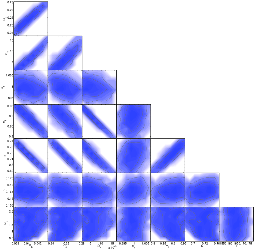
We plot in Fig.4 the results we find for an MCMC run assuming Planck data alone. As we can see the main degeneracies will remain in Planck data, noting the strong negative correlation of and which can be explained by less growth with a cosmology with neutrinos. Specially models in which cannot be ruled out if values of turn out to be near the bottom range allowed by particle physics. The upper limits derived from Planck data alone are better than current estimates for the neutrino mass: marginalising over other parameters they lie around eV (). This result is roughly in accordance with other forecasts (Hu & Tegmark, 1999), where the authors find a lower value of eV () using a Fisher matrix analysis and broadly similar assumptions. In Hu & Tegmark (1999) the assumptions of noise of the Planck experiment were slightly different than the ones assumed here, and their Fisher analysis does not account of any non-Gaussian distribution of the parameters. Ichikawa et al. (2005) claim that if neutrinos have a mass scale smaller than then there is very little useful constraining information in CMB datasets.
We point out here that we have made an important approximation in our analysis. We have assumed that we are in the limit where we have such a small mass for the lowest mass eigenstate, that we can set the masses of the lowest mass eigenstates to zero (the two lowest for a normal hierarchy, and the lowest only for an inverted hierarchy; see Fig. 1). This approximation is valid if the masses are small enough that we are not in the quasi-degenerate scenario. Given that all the scenarios we consider here assume a mass below 0.25 eV, this is a reasonable assumption. We have not considered here the possibility that different neutrino masses may be measurable by cosmological data as this is beyond the capabilities of the surveys we consider.
2.3 Results from LSS and effects of priors.
It was pointed out in Elgarøy & Lahav (2003) that the role of priors is vital in retrieving information about the neutrino mass from cosmological surveys. This is because of the large set of parameters that determines the behaviour of cosmological perturbations and the complicated relation between them. There is for instance a tight correlation between the matter density and the neutrino parameter . This occurs because over most of the evolution of the Universe, neutrinos behave just as cold dark matter, hence it is necessary to know the cold dark matter density well to determine effectively by how much it effectively changes as neutrinos become non-relativistic.
Given that one of the major effects of a high is a strong damping of the power at small scales due to free streaming, it is strongly correlated with the value of . It is very important to measure in order to deduce a neutrino mass. It is possible that the discrepancies between current results that do agree broadly but not in the detail, comes down to the priors used, for instance (Elgarøy et al., 2002) did not assume a varying scalar index in their analysis. They chose to give results for different choices of . One may use theoretical priors to consider only values close to but in doing so one must be wary of the large degeneracy between and .
Most current results rely on priors in one way or another. We argue that in order to obtain a clean measurement of the neutrino mass it will be important to use cosmological data in a way that we are sure that our result in not too prior dependent. We will argue in this paper that a future CMB data set, such as one from Planck, combined with a galaxy survey, such as one from the SKA, can provide the data necessary for a robust analysis of neutrinos via cosmology.
3 Measuring neutrino masses with the SKA
3.1 A back-of-the-envelope calculation
As we have outlined, a measurement of the shape of the power spectrum at large scales as given by Eqn.9 would be able to constrain for the neutrino sector. Here we attempt to estimate the extent to which we would be able to measure this effect with a future large-scale-structure (LSS) survey. In this section we outline a simple back-of-the-envelope calculation to estimate the cosmic volume required, and then in Sec.3.3 we undertake a more detailed calculation that takes into account the full effect that neutrinos have both on LSS and CMB data.
However, data produced by redshift surveys on large scales is often cosmic-variance limited. In this case, the fractional error with which we can measure is proportional to the number of modes present in the survey volume, and hence the accuracy is inversely proportional to the square root of the cosmic volume (Eqn.13).
If we ignore for now the role of priors that, in reality, complicate the analysis (Sec. 3.3), the upper limits from surveys such as the 2dF Galaxy Redshift Survey (2dFGRS) and the SLOAN Digital Sky Survey (SDSS) are around (Tegmark et al., 2006). Hence, a survey with times the cosmic volume would have errors on large scales a factor of -times smaller and therefore would be able to probe eV at the bottom end of the range allowed by particle physics, provided the relation given in Eqn.9 holds. Such an experiment would, by detecting the signal from neutrinos imprinted on the large-scale structure, be able to probe the entire neutrino sector allowed by current particle physics experiments
Furthermore, if we do have such a large volume to search for features imprinted on the galaxy power spectrum, other cosmological parameters will also be accurately determined. The problems with priors and parameter degeneracies that plague current analyses should be much reduced. Current redshift surveys also suffer from the problem of correlated errors on large scales because window functions of these surveys are necessarily narrow in real space, and hence broad in space. An ‘all sky’ survey reaching to very high redshifts would be the optimal way to probe such signals, but we will consider here an, as yet hypothetical, LSS survey reaching to redshift . Such a survey would provide the huge increase in cosmic volume needed to comprehensively probe neutrino properties. For specific calculations we will use simulated LSS datasets from surveys with the SKA, although clearly our conclusions will be valid for any LSS survey with similar reach in sky area, redshift depth and galaxy number density. Further details concerning future redshift surveys with the SKA can be found in the following references: details concerning galaxy number densities in Abdalla & Rawlings (2005); details concerning measurement in Abdalla et al. (2006); a comparison with other future LSS datasets in Rawlings & Abdalla (2006).
3.2 The cosmological imprint of neutrinos in a future LSS data set
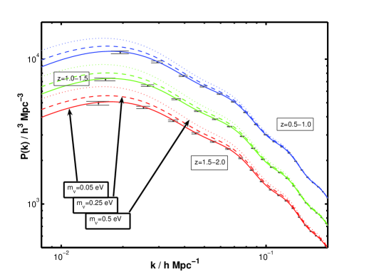
We illustrate in Fig.5 the promise of a future LSS (SKA) survey for detecting the imprint of neutrinos on the power spectrum . We note that we have chosen bins in redshift space which correspond to intervals in comoving space larger than the corresponding to , hence the theoretical error bars plotted are uncorrelated. Fig.5 is the result of a simple analysis in which all other cosmological parameters are fixed at fiducial values and is varied through the neutrino density parameter (using Eqn.6 in a quasi-degenerate scenario with ). We can see clearly that this agrees well with the back-of-the-envelope calculation presented in Sec.3.1, with even models with starting to show significant deviations from the fiducial model which ignores neutrinos.
Another key point illustrated by Fig.5 is the importance of undertaking a LSS survey in independent redshift shells. A common criticism of attempts to constrain from LSS measurements is that the feature being looked for maybe being masked, or even mimicked, by features introduced by the use of galaxies as an indirect probe of the underlying fluctuations. A LSS survey which can probe several redshift shells can give a very good handle on any such systematic errors present in a galaxy redshift survey. One specific worry that has to be addressed is whether any biasing effect from the galaxy power spectrum would be able to produce any scale-dependent modulation mimicking the damping tail of massive neutrinos (Seljak, 2000). First, any worry on this specific issue is attenuated from the theoretical expectation from the halo model (Seljak (2000); Peacock & Smith (2000); and see Abdalla et al. (2006)) that the galaxy bias is, at least on large scales, reliably modelled as a constant multiplicative factor plus a constant additive shot noise. It is only at small scales that this assumption should break down. Hence, the neutrino mass estimate should be robust against this kind of systematic. Second, as illustrated in Fig.5, the huge number of galaxies of an SKA-like LSS survey would allow us to probe the galaxy power spectrum with several galaxy types in each redshift shell, and therefore produce an independent power spectrum for each galaxy type. If we are concerned about any systematic problem due to galaxy bias, we should be able to compare the power spectrum for different galaxy types in each shell. All shells should have the same signal arising from neutrino physics, whereas each power spectrum would be different if there is an effect mimicking the effects of neutrinos because each is made up of samples of galaxies which have different bias and clustering properties. Cole et al. (2006) have shown that it is important to correctly model any scale dependent bias which is luminosity dependent. With a future LSS survey it will be important to have enough galaxies to correctly model this effect. With an SKA survey the number of galaxies will be large enough so that we are able to model the scale dependence of the bias as a function of galaxy properties which we can retrieve from the data, i.e. as a function of hydrogen mass and circular velocity which should correlate to the dark matter mass of the galaxy. There is therefore a better prospect to model a scale dependent bias than may be possible with optical surveys.
However, there is another potential problem that Fig.5 fails to address. We still need to test whether constraints on neutrino parameters are robust to problems induced by degeneracies between cosmological and neutrino parameters. Such degeneracies could make an LSS experiment more heavily reliant on priors than on the data itself, and hence yield misleading forecasts.
3.3 MCMC methods probing a quasi-degenerate scenario with the SKA.
In order to probe the cosmological parameter space for these models we use a Markov Chain Monte Carlo (MCMC) methods in order to obtain a prediction of the posterior probability for a given model and a given future survey. We use a model with neutrinos as a model cosmology and use the following 13 parameters in our MCMC chains: {, , , , , , , , , , , ,}. The first seven parameters are the usual cosmic parameters and the last six parameters are the multiplicative bias and an additive shot noise power arising from the halo model, in each one of the three redshift bins, that we marginalise over.
We will focus on two MCMC-based studies: one which assumes the absolute mass scale for the neutrinos chosen to be the lowest mass which an SKA survey can, on its own, measure sufficiently to discriminate between a normal and inverted hierarchy; another which combines Planck and SKA data on the assumption that the mass scale is , the lowest allowed by particle physics.
3.3.1 SKA-only study at eV.
We first choose to examine whether a survey with the SKA will be able to probe as low as and be able to completely rule out models which have a quasi-degenerate neutrino mass spectrum. We therefore choose a fiducial model which has only two massive neutrinos with the following cosmological parameters {, , , , , , } = {0.04,0.255,0.005,0.72,1.0,0.9,2.0}. We impose an uniform top-hat prior on assuming that the standard model for neutrinos imposes three neutrino eigenstates. The fiducial bias for all the redshift bins has been conservatively set to one but we note that if a larger bias is found, which is likely to be the case, especially in higher redshift bins the significance of the measurements of neutrinos will improve. We assume a fiducial shot noise value equal to one over the number density of galaxies.
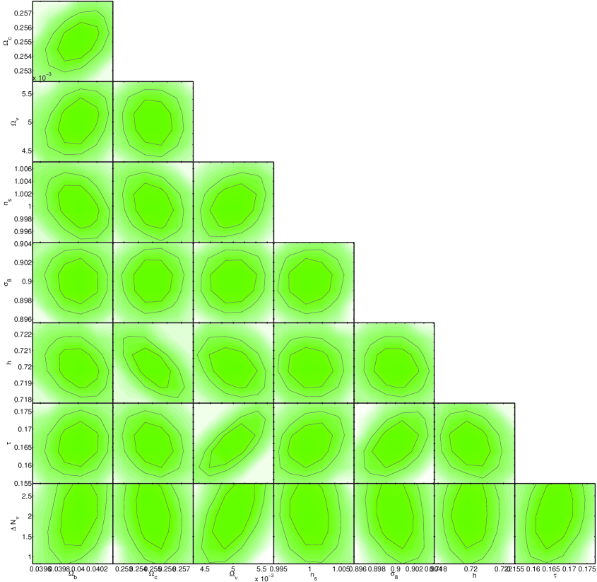
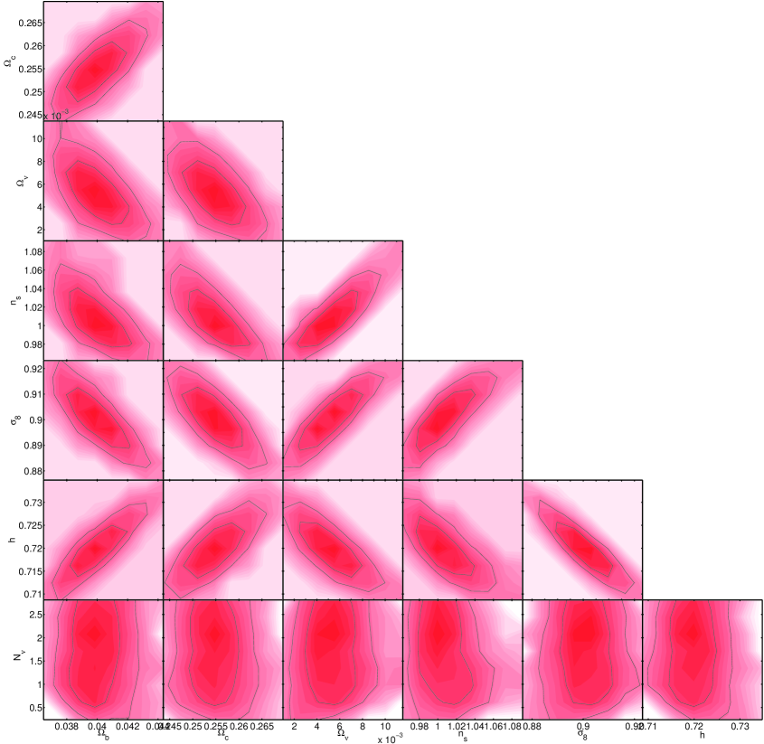
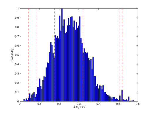
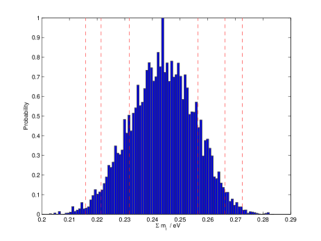
We plot in Fig.6 and Fig.9 the MCMC samples for an analysis following the methods outlined. We note that with this future SKA survey alone, there should be a detection of the absolute mass scale of the neutrino. The measurement of the power spectrum is accurate enough that other parameters are well constrained so stringent priors are therefore unnecessary for a detection of the neutrino signature to be made. We argue that this is of extreme importance for a result to be considered robust not only by the astrophysical community but also by the particle physics community. For such a sample we can estimate the direct forecasted posterior on the sum of the neutrino masses. We plot this in Fig.7 from which the neutrino absolute mass scale can be detected at more than the three sigma level.
3.3.2 SKA plus CMB study at .
It is important to understand and predict how other data will affect the predictions of Sec.3.3.1. Even though we have argued that restrictive priors may be unhelpful when it comes to interpreting how much information is encoded in a given data set, it is certain that additional data sets can provide a huge gain in sensitivity for a given cosmological experiment as has been pointed out by many authors (e.g. Hu et al., 1998).
If we ignore the problems of parameter degeneracy a LSS survey which can get redshifts for sources over out to a redshift of two would be able to reach 0.05 eV (Fig.2). However the problem of parameter degeneracy plagues any interpretation of these data. For instance if we are assessing models which have small values of then the suppression of the power at small scales is very small and can be mimicked by a change in in the primordial power spectrum. Hence a LSS survey would be unable to distinguish between a signal left over from an inflationary phase of the Universe and a signal due to neutrinos.
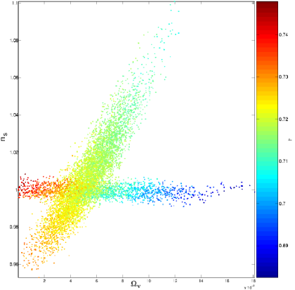
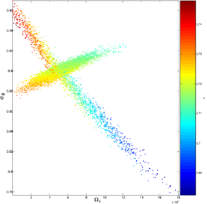
In Fig.9 we see the full posterior probability distributions for the combination of LSS (SKA) and CMB (Planck) experiments. We illustrate in Fig.8 the - degeneracy present in a future SKA survey on its own. This degeneracy is made worst because we have included modes up to a conservative value of of 0.2 . The power spectrum becomes non-linear at larger scales (smaller k) than and if we could find a satisfactory way of modelling these non-linearities we would be able to use these data to help break this degeneracy. However Planck will be able to probe high values by measuring high values in the CMB power spectrum. As gravitational growth is much less advanced at , non-linearities are not an issue and CMB data are therefore also ideal to constrain . As we can see from Fig.8, Planck will measure very well independently of most other parameters. Hence a combination of these two data sets will improve the error bars on the neutrino mass by a factor of five assuming a fiducial model with eV. We plot the improvement on the estimates in Fig.10.
Another degeneracy that plagues estimates of the neutrino mass via cosmological methods is the value of the initial fluctuations which can be parameterised as the value it has at the CMB via or the current strength of the anisotropies parametrised by . Given that one of the effects of a massive neutrino in cosmology is the change in the growth factor for a lengthy period of the history of the Universe, a direct comparison between the scale of anisotropies on the CMB and more locally with redshift surveys can also improve greatly the estimates of the neutrino mass.
We plot in Fig.8 the - degeneracy for CMB and LSS surveys. Whereas for the CMB, growth is responsible for the large degeneracy between and , for the a LSS survey is is the shape of the power spectrum which is mainly responsible for the observed degeneracy, i.e. fixes a weighted integral under , whereas changes the overall shape of . By combining the two estimates a huge improvement can be achieved.
However a poor knowledge of the bias parameter would not allow us to combine these data sets in a consistent way and the improvement would be much smaller. We have assumed that the bias of high redshift galaxies can be measured and marginalised via measurements of modes with different sky orientation, through the influence of redshift space distortions (see Eqn.14). In our MCMC chains the bias is constrained to a few per cent level and marginalised over. For a more realistic simulation we could include other effects such as small scale redshift space distortions. Current spectroscopic surveys with much smaller samples are able to measure the bias to about the several per cent level by measuring bias using higher order statistics such as the bispectrum Verde et al. (2002), so we argue that the assumptions we have made here are not over-optimistic.
However we point out that it is possible that the data at high redshift will allow us to probe linear scales up to a much larger values in which case the constraints coming from LSS alone would be greatly improved. Also a better understanding of non-linearities coming from the halo model as well as N-body simulations (Springel et al., 2005) are very promising, and there are realistic hopes that we could use data from the mildly non-linear regime without introducing large systematic errors and hence improve the constraints shown here.
3.3.3 Directly probing neutrino hierarchies with cosmological data with .
In our analysis of mock future data we have assumed that the number of massive neutrinos is constant. If we assume the standard scenario for neutrinos this can arise in a hierarchical case when the hierarchy is either an inverse hierarchy or a normal hierarchy (Fig.1). If the hierarchy is quasi degenerate, then the number of massive neutrinos will be characterised by and this represent a density of neutrinos equal to 422 million particles per .
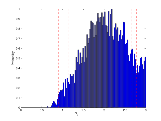
As we stated in the Sec.3.3.2 we have assumed in our fiducial model a number of neutrino which corresponds to an inverted hierarchy where the neutrinos are not all degenerate in mass (Fig.1). By assuming that is a continuous variable we can therefore compare and contrast models which assume a normal hierarchy and models that have an inverted hierarchy. A model with would correspond to an normal hierarchy.
As we ran MCMC chains for LSS (SKA) data alone and CMB (Planck) data alone we noted that for a top-hat prior , which is what one would expect in a standard neutrino scenario without sterile neutrinos or any other exotic relativistic particle that could contribute significantly to the energy density of the Universe, both of these experiments do not constrain significantly. In fact as we can see from the relevant panels of Fig.6 and Fig.4, the prior plays a bigger role in the posterior than the experimental information itself if we consider each experiment independently. It would be more instructive if this were real data to widen the prior allowing more exotic scenarios to be allowed by the model. However, when we combine both experiments we obtain a constraint which is slightly prior dependent but which is now mostly determined by data and this combination of data would yield a measurement of (1) and would reject the value at just under 3. We plot in Fig.11 the expected posterior probability for the value of in this case.
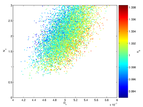
This combination of and would yield invaluable information in order for us to be able to disentangle the origin of the neutrino mass and have a convincing theory which would explain the huge difference between the masses of other particles and the neutrino mass. We plot in Fig.12 the constraints of both of these parameters from a combination of LSS and CMB experiments.
3.4 Indirectly probing neutrino hierarchies with cosmological data at eV.
We have shown that for a fiducial model where and there is a good prospect of a very significant detection of (Secs.3.3.1 and.3.3.2), and a reasonable prospect of a detection of with future SKA data (Sec.3.3.3). The problem is significantly harder if we wish to push the bounds to a neutrino mass of eV which is the limit one would like to attain given that it is the lower limit of the parameter space allowed from particle physics experiments.
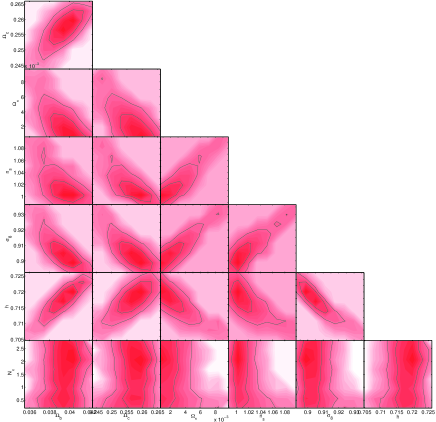
We have run MCMC chains that assumed a fiducial model {,,,,,, } = {0.04,0.259,0.001,0.72,1.0,0.9,2}, together with additional nuisance parameters, in order to test whether the predictions we made hold and to know whether future surveys will be able to push the limits for .
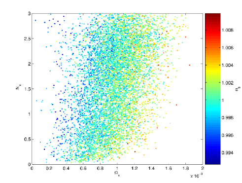
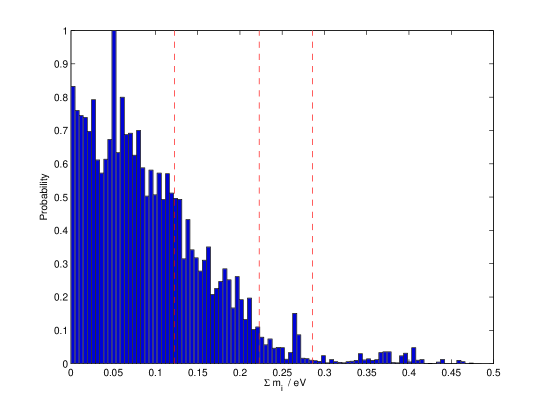
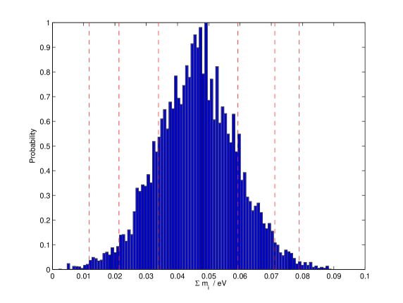
We find that for an SKA survey alone the relevant parameters will not be measured accurately enough to provide strong bounds on the neutrino mass. We plot in Fig.13 the MCMC samples from such a theoretical experiment. We find that a LSS (SKA) survey on its own will not be able to find a signal either from the neutrino density parameter or from the number density of massive neutrinos if . It turns out that the parameter degeneracy is too strong for there to be a clear detection. A 3 upper limit for the neutrino mass would in this case be (95% confidence).
However the addition of CMB data does improve significantly the estimate of at these low masses. As we can see from Fig.14 it would be possible to measure the neutrino mass accurately with if we include both future LSS (SKA) and CMB (Planck) data. This would mean that the entire parameter space that is currently still allowed by current cosmological and laboratory experiments would be probed and a signal from a massive neutrino would be detected.
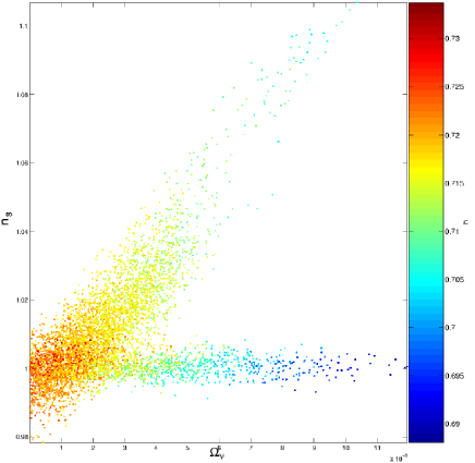
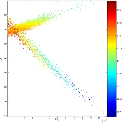
It is possible for us to ask also whether it is possible to detect with this signal. We plot in Fig.15 the posterior from the MCMC samples for the parameters and . Even though the mass density of neutrino can be measured accurately, is totally unconstrained within the priors we have chosen. It would of course with real data make sense to then widen the prior and obtain a sensible error for this parameter. However, with a strong detection of the neutrino mass it is still possible within a certain range to obtain indirect conclusions with regards to the neutrino hierarchy. If an inverted hierarchy is assume then we can simply assume that there are two massive neutrino and ignore the mass of the third neutrino and consider it massless. In this case, given that there is a minimum mass splitting, and we find a total sum of neutrino masses equal to less than twice this value then the hierarchy cannot be inverted. This ‘reductio absurdum’ method implies that if then the hierarchy must be normal.
We conclude that a combined data set comprising LSS (SKA) and CMB (Planck) would be able to detect the signal of a massive neutrino any standard scenario. Furthermore, if the sum of neutrino masses is below 0.1 eV or above 0.25 eV there is a good possibility that cosmological data will be able to prefer one hierarchy strongly. However if the sum of neutrino masses is in the difficult range 0.1 - 0.25 eV then the data we have considered may not be enough for a strong preference to be found with regards to the hierarchy.
4 Concluding remarks
We have shown that future cosmological experiments will be able to detect a signal from a cosmological massive neutrino. This signal would be encoded as a gentle curvature in the galaxy power spectrum correlated with a shift of the CMB temperature and polarisation peaks. We argue that it will be possible to remove any systematics present in data arising from the clustering properties of galaxies by the use of different galaxy types in different redshift bins. Furthermore, data will be available from galaxies with different spatial clustering and hence any systematic effects will be assessed by comparing data sets with galaxies with different clustering and redshift distributions.
We argue that for a clear detection to be made with confidence we need to be sure that any prior used does not affect the results significantly. We find that future cosmological data, both LSS (SKA) and CMB (Planck) data will be accurate and wealthy enough so that priors will play less of a role given that it will be able to measure several key parameters at once including the matter density and the Hubble constant. We find as was already pointed out several times in the literature, a strong complementarity between CMB and LSS data.
Although it is of utmost importance to measure properties of neutrinos directly with particle physics experiments, there are several limitations to these techniques given that the mass scale of neutrinos is extremely small. Therefore other probes from cosmological studies are key to having a more complete picture of neutrino physics. Furthermore, if we are to assess unusual theories such as scenarios where sterile particles are present and have an energy density that influences cosmological data, then there needs to be detailed comparisons between the values drawn from direct particle physics detections and from cosmology.
We argue here that if the mass scale of the neutrino is very small we find ourselves necessarily in a non-degenerate scenario. However if this mass scale is large enough, the spectrum of masses becomes quasi-degenerate and most of the masses are almost equal. Current experiments cannot yet distinguish between these scenarios but may be on the verge of doing so. From a particle physics prospective the absolute mass scale of the neutrino is larger than 0.05 eV and smaller than 2 eV.
We have analysed to what extent neutrino parameters can be recovered by combining future Planck data and a LSS survey, e.g. with the SKA, that would measure redshifts out to over a large fraction of the sky. We conclude that this set of experiments would be sensitive over the entire mass range allowed by current particle physics experiments down to 0.05 eV at the 3 level. We find that even though the mass of the neutrino can be measured for the entire parameter space currently still allowed by experiment, it is harder to measure the number density of massive neutrinos. We find that down to 0.25 eV it is possible to measure the number density well enough to distinguish between a scenario where one or two of the mass eigenstates are massive and hence to be able to distinguish between a normal and an inverted hierarchy.
We have ignored the effects of any varying equation of state of dark energy, assuming that this value will mainly be determined by the angular scale of the wiggles in the power spectrum. This information depends strongly on the value of and very weakly on the value of , hence providing orthogonal constraints as has already been seen in real data (Goobar et al., 2006). Of course could be the real answer.
We have also chosen to use a single value for so that the the running of the spectral index is set to zero. We argue that the degeneracy that will degrade the neutrino sector constraints depends on to first order and on to second order. The Planck satellite is a mission designed to probe the shape of the initial power spectrum to unprecedented accuracy and hence will determine (see Planck ‘blue book’ 111http://www.rssd.esa.int/Planck). .
We have also assumed the initial conditions to be adiabatic pertubations. Although it has been shown that isocurvature perturbations may generate degeneracies with neutrino parameters (Zunckel & Ferreira, 2006), polarisation experiments from Planck will also impose stringent limits on the amount of initial isocurvature. We therefore stress the importance of a high quality CMB mission as well as a deep all-sky redshift survey in order to determine the neutrino parameters, because if this is not the case, limits from LSS alone would be also plagued by degeneracies.
We find that LSS (SKA) and CMB (Planck) data will constrain down to 0.05 eV with an error of around 0.015 eV. If is indeed below 0.1 eV it will be possible to rule out an inverted hierarchy indirectly given that having an inverted hierarchy with such small is in contradiction with atmospheric neutrino experiments. We therefore conclude that if the neutrino mass lies between 0.05 and 0.1 eV or above 0.25 eV it should be possible to distinguish clearly between the normal or inverted hierarchies. However, it will not be possible to do so clearly if the mass lies between 0.1 and 0.25 eV. These results may be modified and improved, if a large range in data points can be used, and specially if higher values can be included in the analysis by virtue of improved modelling of non-linear fluctuations.
It is of great importance that cosmological experiments provide us with the same answers and parameters as particle physics experiments. Put another way, it may eventually be possible to measure any exotic sterile particles that would contribute to the cosmic background of relativistic particles and hence influence but which could not be detected by particle physics. We argue that it is likely to be possible to constrain strongly any of these scenarios given that the data will be sensitive down to eV and .
Acknowledgements.
We are very grateful for useful discussions with Steve Biller, Chris Blake, Sarah Bridle, Joanna Dunkley, Pedro Ferreira and Will Percival. We thank the Gemini Project and PPARC for a Studentship (FBA) and PPARC for a Senior Research Fellowship (SR). This research has been undertaken as part of the SKA Design Study SKADS.
References
- Abdalla et al. (2006) Abdalla F. B., Blake C. A., Rawlings S., 2006, MNRAS to be submitted
- Abdalla & Rawlings (2005) Abdalla F. B., Rawlings S., 2005, MNRAS, 360, 27
- Alcock & Paczynski (1979) Alcock C., Paczynski B., 1979, Nat, 281, 358
- Ballinger et al. (1996) Ballinger W. E., Peacock J. A., Heavens A. F., 1996, MNRAS, 282, 877
- Blake & Glazebrook (2003) Blake C., Glazebrook K., 2003, ApJ, 594, 665
- Bucher et al. (2002) Bucher M., Moodley K., Turok N., 2002, Phys. Rev. D, 66, 023528
- Cole et al. (2006) Cole S., Sanchez A. G., Wilkins S., 2006, astro-ph/0611178
- Dunkley et al. (2005) Dunkley J., Bucher M., Ferreira P. G., Moodley K., Skordis C., 2005, MNRAS, 356, 925
- Eisenstein et al. (1999) Eisenstein D. J., Hu W., Tegmark M., 1999, ApJ, 518, 2
- Elgarøy & Lahav (2003) Elgarøy Ø., Lahav O., 2003, Journal of Cosmology and Astro-Particle Physics, 4, 4
- Elgarøy & Lahav (2005) Elgarøy Ø., Lahav O., 2005, New Journal of Physics, 7, 61
- Elgarøy et al. (2002) Elgarøy et al. 2002, Physical Review Letters, 89, 061301
- Feldman et al. (1994) Feldman H. A., Kaiser N., Peacock J. A., 1994, ApJ, 426, 23
- Fukuda et al. (1996) Fukuda et al. 1996, Physical Review Letters, 77, 1683
- Fukugita et al. (2006) Fukugita M., Ichikawa K., Kawasaki M., Lahav O., 2006, Phys. Rev. D, 74, 027302
- Glazebrook & Blake (2005) Glazebrook K., Blake C., 2005, ApJ, 631, 1
- Goobar et al. (2006) Goobar A., Hannestad S., Mörtsell E., Tu H., 2006, Journal of Cosmology and Astro-Particle Physics, 6, 19
- Guth (1981) Guth A. H., 1981, Phys. Rev. D, 23, 347
- Hannestad (2003) Hannestad S., 2003, Phys. Rev. D, 67, 085017
- Hu et al. (1998) Hu W., Eisenstein D. J., Tegmark M., 1998, Physical Review Letters, 80, 5255
- Hu & Haiman (2003) Hu W., Haiman Z., 2003, Phys. Rev. D, 68, 063004
- Hu & Tegmark (1999) Hu W., Tegmark M., 1999, ApJ Lett., 514, L65
- Ichikawa et al. (2005) Ichikawa K., Fukugita M., Kawasaki M., 2005, Phys. Rev. D, 71, 043001
- Kaiser (1987) Kaiser N., 1987, MNRAS, 227, 1
- Kayser (2005) Kayser B., 2005, SLAC Lecures 2004
- Lesgourgues & Pastor (2006) Lesgourgues J., Pastor S., 2006, Phys. Rept., 429, 307
- Lewis & Bridle (2002) Lewis A., Bridle S., 2002, Phys. Rev. D, 66, 103511
- Lewis et al. (2000) Lewis A., Challinor A., Lasenby A., 2000, ApJ, 538, 473
- Maltoni et al. (2004) Maltoni M., Schwetz T., Tórtola M., Valle J. W. F., 2004, hep-ph/0405172, New Journal of Physics, 6, 122
- Peacock & Smith (2000) Peacock J. A., Smith R. E., 2000, MNRAS, 318, 1144
- Peacock et al. (2001) Peacock et al. 2001, nat, 410, 169
- Rawlings & Abdalla (2006) Rawlings S., Abdalla F. B., 2006, Conference Procedings ‘On the Pathway to the SKA’
- Seljak (2000) Seljak U., 2000, MNRAS, 318, 203
- Seljak & Zaldarriaga (1996) Seljak U., Zaldarriaga M., 1996, ApJ, 469, 437
- Seljak et al. (2005) Seljak et al. 2005, Phys. Rev. D, 71, 103515
- Seo & Eisenstein (2003) Seo H.-J., Eisenstein D. J., 2003, ApJ, 598, 720
- Spergel et al. (2003) Spergel et al. 2003, ApJS, 148, 175
- Spergel et al. (2006) Spergel et al. 2006, ArXiv astro-ph/0603449
- Springel et al. (2005) Springel V., White S. D. M., Jenkins A., Frenk C. S., Yoshida N., Gao L., Navarro J., Thacker R., Croton D., Helly J., Peacock J. A., Cole S., Thomas P., Couchman H., Evrard A., Colberg J., Pearce F., 2005, nat, 435, 629
- Tegmark et al. (2006) Tegmark et al. 2006, ArXiv astro-ph/0608632
- Verde et al. (2002) Verde et al. 2002, MNRAS, 335, 432
- Zunckel & Ferreira (2006) Zunckel C., Ferreira P. G., 2006, astro-ph/0610597