An Inhomogeneous Model Universe Behaving Homogeneously

Abstract

We present a new model universe based on the junction of FRW to flat Lemaitre-Tolman-Bondi (LTB) solutions of Einstein equations along our past light cone, bringing structures within the FRW models. The model is assumed globally to be homogeneous, i.e. the cosmological principle is valid. Local inhomogeneities within the past light cone are modeled as a flat LTB, whereas those outside the light cone are assumed to be smoothed out and represented by a FRW model. The model is singularity free, always FRW far from the observer along the past light cone, gives way to a different luminosity distance relation as for the CDM/FRW models, a negative deceleration parameter near the observer, and correct linear and non-linear density contrast. As a whole, the model behaves like a FRW model on the past light cone with a special behavior of the scale factor, Hubble and deceleration parameter, mimicking dark energy.

1 Introduction

Already in 1982, long before the detection of acceleration of the universe and suggestions in favor of inhomogeneous models as explanation for this novel cosmic effect, Bahram published a work in collaboration with Hossein Partovi Bahram84 in which they developed a model with radial inhomogeneities as a first step toward a framework for comparison with observations. The paper did not get much attention due to the lack of observational evidence. The supernovae data indicating the acceleration of the universe Riess98 ; Perl99 caused a revival of the idea of an inhomogeneous universe. This time the authors mainly considered Lemaitre-Tolman-Bondi (LTB) solution of the Einstein equation as the model universe Lemait33 ; Tolman34 ; Bondi47 and indicated a change in the luminosity distance relation towards explaining the acceleration of the universe due to the supernovae data (see Celer06 and Mansouri05 for references). Now, most of the authors consider the inhomogeneous solutions of the Einstein equations as an alternative to FRW model of the universe (see Biswas06 ,Celer07 and the references there). There is, however, another way of understanding the inhomogeneity and the interpretation of data on our past light cone. We know already from many simple examples that cutting a manifold along a null hypersurface and pasting it again after some warping we may get gravitational shock or impulsive waves along the null hypersurface even in an otherwise Minkowski spacetime. This has been nicely shown in the paper by Penrose Penrose72 . The cut-and-paste method is an elegant way to understand many astrophysical phenomena using exact $C^{0}$ solutions of the Einstein equations. These solutions are usually $C^{3}$ everywhere except across a null hypersurface of the junction. Nevertheless, the inhomogeneous models of the universe as partial explanation of dark energy, as Germans would say, are just beginning to be salonfähig. The task force for dark energy DETF does not consider inhomogeneities as a possible explanation for dark energy. The first review or policy document in which the inhomogeneity is explicitly mentioned as a possible way to understand the acceleration of the universe seems to be “The Newsletter of the Topical Group in Gravitation …” APS .

We will report here on a model universe based on a cut-and-paste technology of matching an inhomogeneous model to a FRW model universe across the past light cone of the observer. The philosophy behind it is the following. After the decoupling era the universe, being almost in a global FRW state, begin to develop as a matter dominated universe witnessing a growth of structures. The structures do not change the global homogeneous character of the universe, but locally the inhomogeneities begin to grow. Any local observer, in a globally Copernican view, will feel the effects of inhomogeneities in the course of time. Needless to say that the inhomogeneities outside his past light cone has no such effect and he may always assume that everything outside his past light cone is effectively homogeneous and is to be considered as a FRW model. On the contrary, the inhomogeneities in his vicinity within the light cone, which grows in time, may have direct cosmological consequences on his observations. These effects have to be increasing with decrease of the redshift on the past light cone. Therefore, we are faced with a model universe in which the past light cone of the observer is a boundary between a FRW model universe and an inhomogeneous model which goes to a FRW with increasing $z$, to match the requirement of almost FRW everywhere before the onset of nonlinearities in the structures. For simplicity, we assume a LTB metric for the inhomogeneous part. The matching should be such that no shear is produced on the light cone as required for a simple boundary of observation. We will see that as a matching condition the light cone behaves as if we are in a FRW homogeneous model, but somehow dilated, mimicking a dark energy not existent in either FRW or LTB solutions on either side of the light cone. We have called this model Structured FRW (SFRW), as opposed to the familiar homogeneous FRW model of the universe Mansouri05 .
The model we are considering is related to the Swiss Cheese model but differs from it substantially. The Swiss cheese model of cosmology, first suggested by Kantowski in 1969 Kant69 , studies the effects of local inhomogeneities in the FRW models on the propagation of light through an otherwise homogeneous and isotropic universe. Kantowski’s model is constructed by taking the Friedman model ($p=\Lambda=0$), randomly removing co-moving spheres from the dust, and placing Schwarzschild masses at the center of the holes. The remaining Friedman dust is interpreted as dust between clumps, and the point masses are interpreted as inhomogeneities.
The paper has essentially two parts. In part one, we study in detail the flat LTB solution of Einstein equations, its singularities, and the bang time. This is just to get more insight how we are going to use the LTB which differs substantially from its usage in cosmology in the recent literature. This is done in section 2 where we have written down the necessary formulas to define the LTB metric and their corresponding Einstein equations, the bang time and singularities, appropriate choice of the bang time, the past light cone, and the place of singularities within it. Part one may be skipped by those familiar with the LTB solution of the Einstein equations, except for the numerical results showing the place of singularities. In part two we define the model and study its cosmological consequences. Section 3 is devoted to the explicit definition of our SFRW model universe. In section 4 we look at the cosmological consequences of our model, the age of the universe, luminosity distance, deceleration parameter, and the density contrast, followed by a section on conclusions.

2 Flat LTB solution and related cosmological quantities

We constrain ourselves to the so-called flat or marginally bound LTB models. These are solutions of Einstein equations described by the metric

$$ds^{2}=-c^{2}dt^{2}+R^{\prime\,2}\,dr^{2}+R^{2}(r,t)(d\theta^{2}+\sin^{2}\theta d\phi^{2}),$$ (1)

in which overdot and prime (will thereafter) denote partial differentiation with respect to $t$ and $r$, respectively. The corresponding Einstein equations turn out to be

$$\dot{R}^{2}(r,t) = \frac{2GM(r)}{R},$$ (2)

$$4\pi\rho(r,t) = \frac{M^{\prime}(r)}{R^{2}R^{\prime}}.$$ (3)

The density $\rho(r,t)$ is in general an arbitrary function of $r$ and $t$, and the integration time-independent function $M(r)$ is defined as

$$M(r)\equiv 4\pi\int^{R(r,t)}_{0}\rho(r,t)R^{2}dR=\frac{4\pi}{3}\overline{\rho}(r,t)R^{3},$$ (4)

where $\overline{\rho}$, as a function of $r$ and $t$, is the average density up to the radius $R(r,t)$. The metric (1) can also be written in a form similar to the Robertson-Walker metric. The following definition

$$a(t,r)\equiv\frac{R(t,r)}{r}\,\,,$$ (5)

brings the metric into the form

$$ds^{2}=-c^{2}dt^{2}+a^{2}\left[\left(1+\frac{a^{\prime}r}{a}\right)^{2}dr^{2}+r^{2}d\Omega^{2}\right].$$ (6)

For a homogeneous universe $a$ doesn’t depend on $r$ and we get the familiar Robertson-Walker metric. The corresponding field equations can be written in the following familiar form

$$\big{(}\frac{\dot{a}}{a}\big{)}^{2}={G\over 3}\frac{\rho_{c}(r)}{a^{3}},$$ (7)

where we have introduced $\rho_{c}(r)\equiv\frac{6M(r)}{r^{3}}$ indicating a quasi comoving $r$-dependent density. These are very similar to the familiar Friedman equations, except for the $r$-dependence of different quantities. The solutions to the field equations can be written in the form

$$R(r,t) = \left[\frac{9GM(r)}{2}\right]^{1\over 3}\left[t-t_{n}(r)\right]^{2\over 3},$$

$$a(r,t) = \left[\frac{3}{4}\,G\rho_{c}(r)\right]^{1\over 3}(t-t_{n}(r))^{2\over 3}.$$ (8)

Now we choose the coordinate $r$ such that

$$M(r)=\frac{4\pi}{3}\rho_{c}r^{3},$$ (9)

where $\rho_{c}$ is a constant Biswas06 . To adapt this metric to observational data we need to know the backward light cone, the luminosity distance, the corresponding Hubble parameter, the deceleration parameter, the jerk, and the equation of state parameter $w$. We start with the radial light rays. The null geodesic corresponding to radially inward rays is given by

$$cdt=-R^{\prime}(r,t)dr.$$ (10)

Assuming the redshift $z$ as the parameter along the past light cone, we obtain Celer00

$$\frac{dr}{dz}=\frac{c}{(1+z)\dot{R}^{\prime}(r,t(r))},$$ (11)

and

$$\frac{dt}{dz}=\frac{-R^{\prime}(r,t(r))}{(1+z)\dot{R}^{\prime}(r,t(r))},$$ (12)

where $t(r)$ is evaluated along the rays moving radially inward according to (10). The luminosity distance is then given by

$$D_{L}(z)=(1+z)^{2}R.$$ (13)

Definition of the Hubble function is not without ambiguity in the LTB models. The reason is $r$ and $t$ dependence of the “scale factor $a$” Moffat05 ; Moffat06 . Depending on the use of the metric coefficients $R$ or $R^{\prime}$ we may define $H_{R}=\frac{\dot{R}}{R}\,$ or $H_{R^{\prime}}=\frac{\dot{R}^{\prime}}{R^{\prime}}$ as the Hubble parameter, which are different in general. We may also define a Hubble parameter as the expansion rate along the light cone Vander06 . It gives us a quantity which is easy to compare with the observations. Once we have the LTB-luminosity distance from (13), we interpret it as a distance in an effective FRW universe. Assuming the relation

$$D_{L}(z)=(1+z)\int_{0}^{z}\frac{dz^{{}^{\prime}}}{H(z^{{}^{\prime}})}\,\,,$$ (14)

we invert it to define

$$H(z)=\left[\frac{d}{dz}\frac{D_{L}(z)}{1+z}\right]^{-1}.$$ (15)

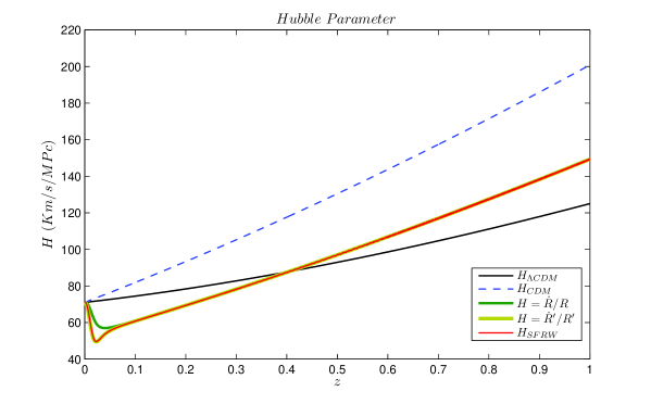
Note that in our structured FRW model this definition corresponds to the Hubble parameter of the FRW background outside the past light cone. Therefore, in general, we may have three different definitions of the Hubble parameter. It has been shown, however, that in the case of glued LTB to FRW along a null hypersurface the three definitions coincide khakshour07 . A numerical comparison is given in section 4.4 and Fig.14
The associated deceleration parameter is then defined as

$$q(z)=-1+\left[\frac{1+z}{H(z)}\right]\frac{dH(z)}{dz},$$ (16)

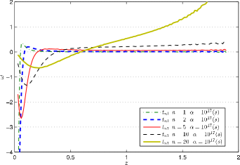
and the effective state parameter

$$w\equiv\frac{2}{3}[q(z)-{1/2}]=\frac{2(1+z)}{3}\frac{d}{dz}\ln\left[\frac{H(z)}{(1+z)^{3/2}}\right]\,\,.$$ (17)

In addition, we may define the jerk as in a FRW universe Mobasher04 ; Sahni03 :

$$j=\frac{\dot{\ddot{a}}}{a}(\frac{\dot{a}}{a})^{-3}=\frac{(a^{2}H^{2})^{\prime\prime}}{2H^{2}},$$ (18)

where prime means derivative with respect to the argument $a$, and substitute an effective scale factor to obtain the corresponding value for our LTB based model. In this way we have a simple way to compare any LTB model with an effective FRW universe and also with the observational data. We may consider jerk as an alternative to $w$ for parametrization of the dark energy. In our case it is to be considered as another way of interpreting inhomogeneities in terms of an effective FRW cosmology.
We will see in section 3 that the effective FRW cosmological parameters defined here are the exact FRW quantities for our SFRW model on the light cone and that different Hubble parameter definitions for the LTB metric coincide with each other and are the same as the Hubble parameter of the background FRW on the light cone.

2.1 Bang time and singularities

The singularities of LTB metric, which are more sophisticated than in the case of the Robertson-Walker metric, have been discussed extensively in the literature (see for example Vander06 , Christo84 , Newman86 ). Vanishing of each of the metric functions and its derivatives $R,R^{\prime},\dot{R},\ddot{R},\dot{R}^{\prime},\newline R^{\prime\prime}$ may lead to different singularities. In a general LTB metric there is another singularity, the event horizon, related to zero of $1+E$, where $E(r)$ is the energy function of the LTB metric, absent in our flat LTB case. Vanishing of $R^{\prime\prime}(t,r=0)$ leads to the so-called central weak singularity in LTB models studied in Vander06 . For this central singularity in a flat LTB model to be absent one must have Vander06

$$t_{n}^{\prime}(0)=0.$$ (19)

In selecting a bang time we will take this into consideration and will avoid those violating this condition. The place of the other singularities, irrespective of its cosmological significance, are summarized as follows:

$$R^{\prime},R^{\prime\prime},\dot{R},\dot{R^{\prime}}=\infty\hskip 14.22636pt\longrightarrow\hskip 14.22636ptt=t_{n}\,\,,$$

$$R=0\hskip 65.44142pt\longrightarrow\hskip 14.22636ptt=t_{n}\,\,,$$

$$R^{\prime}=0\hskip 62.59596pt\longrightarrow\hskip 14.22636ptt=t_{n}+\frac{2}{3}rt^{\prime}_{n}\,\,,$$ (20)

$$\dot{R^{\prime}}=0\hskip 62.59596pt\longrightarrow\hskip 14.22636ptt=t_{n}-\frac{1}{3}rt^{\prime}_{n}\,\,,$$

$$R^{\prime\prime}=0\hskip 59.75095pt\longrightarrow\hskip 14.22636ptt=\frac{3rt_{n}t^{\prime\prime}_{n}+6t_{n}t^{\prime}_{n}-r{t^{\prime}_{n}}^{2}}{6t^{\prime}_{n}+3rt^{\prime\prime}_{n}}.$$

The sign of $t^{\prime}_{n}$, as it may be seen from the above relations, plays an important role in the discussion of the singularities. Taking note of these singularities, we will construct our model such that none of the singularities is on the light cone and all of them are far from the region where the LTB metric is effective.

2.2 Choice of the bang time

According to SFRW model of the universe, the cosmological principle is valid. The universe from the point of view of each observer looks the same: inhomogeneous locally but homogeneous far from the observer and everywhere outside its past light cone. Of course, outside the light cone we have everywhere the local inhomogeneity which may affect us in future, but it is assumed to be smoothed out to a FRW homogeneous universe, as it is always assumed in the familiar FRW model of the universe. The difference is on the light cone and in the vicinity of the observational point, where we do not want to assume the smearing out of inhomogeneities and would like to model it using a flat LTB solution of the Einstein equations, being glued to the outside flat FRW metric khakshour07 .
To formalize this requirement, we fabricate a bang time so that for $r$ greater than a fiducial distance, say $nL$ of the order of magnitude 100 MPc, the metric goes over to FRW, i.e. $t_{n}\rightarrow const$ for $r\gg nL$. Here we assume $L=100$ MPc and leave $n$ to be determined by the observation. For numerical calculation, we therefore define a dimension-less co-moving distance $r^{\prime}=\frac{r}{nL}$. For the sake of simplicity we rename from now on $r^{\prime}$ as $r$. Our coordinate $r$ is now dimensionless and scaled by the inhomogeneity scale $nL$. But note that we may use $r$ for the comoving coordinate or the scaled version of it interchangeably according to the context it is used! Now, for the bang time to have the desired property, we may write it in the following general form:

$$t_{n}=\frac{\alpha}{p(r)+1+q({1\over r})},$$ (21)

where $p$ and $q$ are polynomials in their arguments having no constant and linear term. The time factor $\alpha$ is another constant of the model in addition to inhomogeneity parameter $n$. It is obvious that for $r\ll 1$ the bang time approaches a constant, in fact zero for $q\neq 0$, and for $r\gg 1$ it approaches a constant, zero again for $p\neq 0$, meaning that for large $r$ we have effectively FRW metric again. Note that large $r$ will corresponds in our case to redshifts bigger than 1. To see the cosmological effects of polynomials like $p(r)$ we restrict it to powers of up to $r^{4}$. On the other hand, it is easily seen that large powers of $1\over r$ have not much effect and we can ignore them within the scope of this paper. We, therefore, ignore them altogether to concentrate on the most significant cases and effects. Now, consider just the following two cases:

$$t_{n1} = \frac{\alpha}{r^{2}+1}$$ (22)

$$t_{n} = \frac{\alpha}{r^{4}+r^{2}+1}\,.$$ (23)

These bang times are just two examples of non-singular cases we will concentrate on. In fact, there are many choices leading to almost FRW for large z, as we have tested numerically. They are, however, typically mal-behaved as far as singularities, density contrast, or deceleration is concerned, as it is the case with $t_{n}=\frac{\alpha r^{2}}{1+r^{2}}$ suggested in Vander06 . We will see that the bang time suggested in this paper is free of any singularity on the light cone and reflects a reasonable behavior of the luminosity distance and the deceleration.
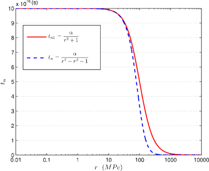
We have plotted the behavior of $t_{n}$ and $t_{n1}$ as a function of $r$ in Fig. 2. Both bang time functions decay very rapidly to zero, which is equivalent to rapid decay of the LTB metric to FRW. Therefore, it reflects the desired feature of SFRW. The $t_{n1}$, however, leads to singular behavior at the light cone for $z$-vlaues larger than $600$. That is why we prefer to work with $t_{n}$. In both cases, however, as it is shown in the following sections, the difference between LTB and FRW is almost negligible for redshifts $z>1$.

2.3 Past light cone and the place of singularities in the flat LTB model

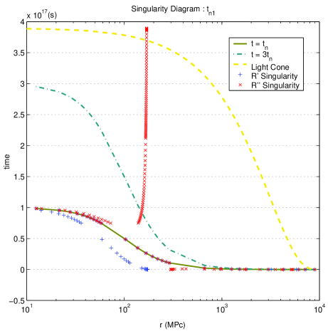
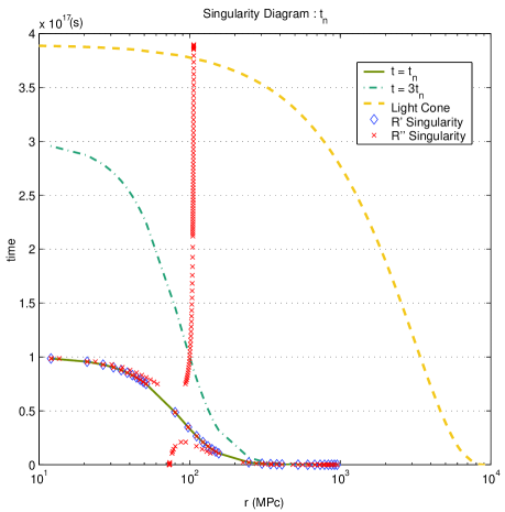
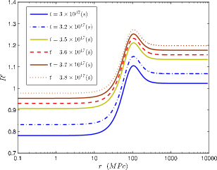
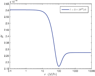
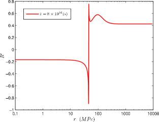
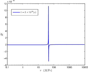
There are many papers dealing with singularities of the LTB metric. It is claimed that LTB metrics have either a weak singularity at the origin or do not lead to an acceleration Flan05 . Here we report on the singularities of $t_{n}$ and $t_{n1}$ as defined above, just as two examples of bang time being non-singular at the origin. The question of acceleration is dealt with in the next section. In Figs. 3 and 4 we have plotted our past light cone and different singularities within it for $t_{n}$ and $t_{n1}$. The singular points of $R^{\prime\prime}$ are also sketched in the mentioned figures. This curve intersects the past light cone on a point which corresponds to a local maximum of $R^{\prime}$ as can be seen from Figs. 5 and 7, and none of the metric invariants, including that of Kretschman, have a singularity at this event. Therefore, we notice that all singularities are within the light cone, well before the time $t=\alpha$, and well outside the vicinity of the light cone in the region where we have effectively FRW again.

Figure 1: Observers A and B have the same picture of the universe: affected by the local inhomogeneities in their vicinity ( above the $z=1$ plane); Outside their past light cone and far from the observer points A and B, the universe seems homogeneous.

3 Definition of the model: Structured FRW Universe

We are used to the Swiss cheese model as a random distribution of over- and under-dense regions in a constant time slice of the space-time, a constant time picture that does not take into account the realities of the observations along the past light cone and the possible evolutionary effects. We intend to modify this picture taking into account that all our observations are along the past light cone, and these observations are not affected by the events outside it.
Let us accept the cosmological principle according to which all observers have the same picture of the universe. As the structures are effectively influencing the universe after the last scattering surface, our goal is to model the matter dominated and pressure-less universe. The universe before the last scattering surface is radiation dominated and structure-less, i.e. it is represented by a FRW metric. After the last scattering and with the growth of structures, our model gradually deviates from the simple CDM/FRW universe in the following way. We will use a combination of FRW and LTB metrics connected to each other along the past light cone in a specific manner. Contrary to the familiar concept of using LTB metric to represent over- or under-density bubbles in the time constant slices of the universe in many papers published in the last years, we use it in a light cone adapted way. We will see that due to our model construction the effect of LTB inhomogeneities vanishes on the light cone and we encounter another effective FRW which differs from the CDM/FRW, although we start with a CDM/FRW in combination with a pressure-less LTB.
The universe is assumed to be globally FRW, but structured locally. Hence, any observer sees the universe in the following way: outside his past light cone, which is not observable to him, we assume the universe to be FRW, i.e. local inhomogeneities outside the light cone are assumed to be smoothed out and the effective metric is FRW. Note that the only use of this assumption is the induced Hubble constant on the light cone. Now, to implement the effect of the local inhomogeneities in the spirit of SFRW model, we assume the metric on the past light cone and its vicinity to be LTB. to define the vicinity we note that the order of magnitude of inhomogeneities is given by $nL$. Now at any $z-$value, the vicinity of the light cone can be determined according to the size of horizon. In fact, we are only concerned with the light cone behavior of the metric in this paper. In a following paper we will define the vicinity more precisely to study the averaging process of the Einstein equations and answer the question of the backreaction of inhomogeneities, its pitfalls, and how to make sense of it khosravi07 . At any point outside this region the observer sees on the average, a FRW homogeneous universe again. Although, FRW and LTB could in principle be any of the three cases of open, flat, or close, it has been shown in khakshour07 that the only meaningful matching of these two spaces along a null boundary is a flat-flat case. 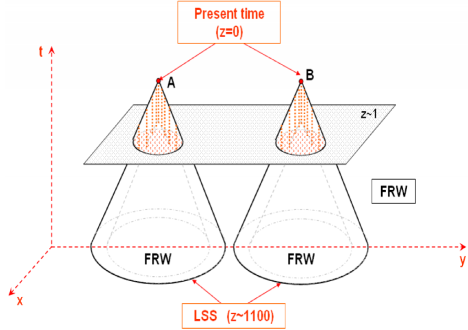In addition, due to the cosmological preferences we will assume both metrics to be flat (Fig. 1).
Note the philosophy behind this picture: The universe is everywhere locally inhomogeneous, but homogeneous at large. Any observer, according to the cosmological principle, has the same picture. Now, he makes his model according to these rules: universe outside his past light cone, i.e. regions of the universe that has not influenced his past, is FRW. Locally, i.e. not far along the past light cone or for small $z$-values which will turn out to be of the order of $z=1$, the observer sees a flat LTB on and within it. Far on the light cone and within it the model tends to be a homogeneous FRW universe again. This is of course in contrast to the usual assumption in the recent literature that the LTB represents bubbles of inhomogeneities.
Now, let us assume the bang time to be

$$t_{n}=\frac{\alpha}{r^{4}+r^{2}+1},$$ (24)

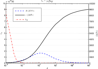
where $r$ is scaled to $nL$. We will alternatively use the comoving coordinate $r$ in the scaled form or not, and the reader may simply see from the context which one is meant. The constant $\alpha$ has the dimension of time. We have, therefore, two model parameters $n$ and $\alpha$ to be determined by observation. Fig. 9 shows $t_{n}$ as a function of the redshift $z$, using (11). We have plotted $r$ and $R$ as a function of $z$ in the same diagram to see the coordinate, or redshift for which our LTB metric is essentially FRW. Obviously, the value $z\approx 1$, corresponding to $r\approx 10$ and $t\approx 2\alpha$, is the boundary of transition from LTB to FRW. The inhomogeneity scale $r\approx 10$, or roughly 1000 Mpc, corresponds to the physical length $\approx 1$ Mpc at the time of the last scattering for $z\approx 1100$. Although the transition point is at a relatively small $z$, we can follow the effect of inhomogeneity up to the last scattering surface at $z\approx 1100$. The bang time is zero almost everywhere, except in our vicinity. Therefore, if the inhomogeneity has any effect, it must show up at our time, in accordance with the cosmological coincidence.

Now, for this bang time (24) we have

$$t^{\prime}_{n}|_{r=0}=0.$$ (25)

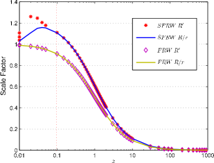
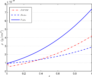
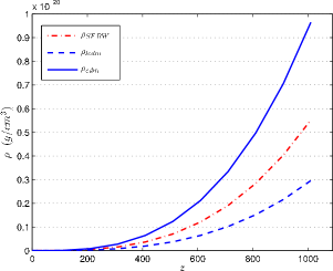
Therefore, we do not expect any weak singularity at the origin Vander06 . In fact, for the LTB domain with this bang time, we have no singularity at all, as it is shown in Fig. 3. Vanishing of $R^{\prime\prime}$ at the light cone and its vicinity indicates a maximum of $R^{\prime}$ for $t=const.$ which reflects a feature of expanding layers. No invariant of the metric has a singularity within the domain of our interest. The singularity $t=3t_{n}$ which appears in the Kretschman invariant is well outside the region of our interest as shown in Fig. 3. We have also plotted in Fig. 5, $R^{\prime}$ as a function of $r$ for some fixed values of time to have a better understanding of variation of the LTB metric function. Note the behavior of $R^{\prime}$ near its maximum values where $R^{\prime\prime}$ vanishes and compare it with Fig. 3. The behavior of the LTB scale factor $R/r$ and the metric function $R^{\prime}$, for the sake of comparison the FRW scale factor for the CDM case ($\alpha=0$) as a function of $z$, is depicted in Fig. 10. The density as a function of redshift is also plotted in Fig. 11 and Fig. 12 for different ranges of $z$.

4 Cosmological consequences of SFRW and observational data

We are now in a position to look at different cosmological consequences of the model. Angular distance and the luminosity distance are given implicitly by the equations (11 - 13). We have to integrate from $z=0$ to the last scattering surface. The definition of the last scattering surface is a delicate problem. Its familiar value $z\approx 1100$ is based on a FRW model. But our SFRW model tends to a FRW at early times. Therefore, to match the SFRW at early times to a radiation dominated FRW we have to have the same age for the universe at the last scattering surface. This fixes the $z$-value in SFRW, which may differ from the one in FRW. It turns out, that for our choice of the bang time the difference is sensitive to the model parameters. Note, however, that for many other choices of the bang time there is no meaningful matching to the radiation dominated universe irrespective of any choice of the parameters. For the range of parameters we are considering, i.e. $0.1<n<3$ and $\alpha\approx 1$ ( in scale of $10^{17}s$) , the difference is negligible and we can fix the last scattering surface at $z\approx 1100$. Before going into its detail, we have to fix another constant of the model, namely $\rho_{c}$. It is determined by the value of the scale factor of the universe at the last scattering surface. Taking it the same as that of FRW at the age of $\approx 10^{13}~{}s$, we arrive at $\rho_{c}\approx 10^{-30}g/cm^{3}$ or $10^{-37}$ in geometrical units.

4.1 Angular distance and the age problem

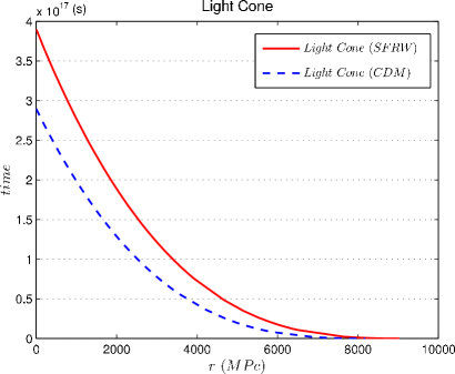
We have fixed now all the constants of the model. The last scattering surface is defined now by $z=1100$, corresponding to the cosmic time $t\approx 10^{13}s$. Integrating the (12), we end up with Fig. 13 for the light cone. For comparison, we have also plotted the CDM/FRW light cone for the same redshift interval. The age of the universe at the last scattering surface is almost the same for both models. Therefore, the value of time for $z=0$ determines the age of the universe in SFRW. It turns out to be $4/3$ of the age in FRW, i.e. $t=3.9\alpha=15\times 10^{9}$ years. Therefore, there is no age problem in the model: the age of the universe in our model is well above any estimation we have in astrophysics and cosmology Carretta00 (see Fig. 13). The angular distance defined by $R(r,t)$ as a function of $z$ is plotted in Fig. 9.

4.2 Luminosity distance

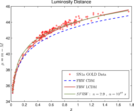
The model is now completely determined. The last scattering surface, having the same age in SFRW and FRW, corresponds to $z\approx 1100$. But as we have seen in the last section, the age of the universe is $4/3$ of that in FRW. Now, we can integrate the equations (11 - 13) to obtain the luminosity distance. Fig. 15 shows the luminosity distance as a function of $z$.
For the sake of completeness and more insight in the models under consideration, we have listed the results of likelihood analysis for the luminosity distance of type Ia supernovae (SNe Ia - GOLD samples Mobasher06 ) given different forms of the bang time $t_{n}$ in the table 1 ( assuming $nL\simeq 100Mpc$ and $\alpha=10^{17}~{}s$).

$p(r)$	$\chi^{2}$ (for 182 SNe Ia)
$r^{4}+1$	255
$r^{4}+r^{2}+1$	265
$r^{2}+1$	226
$r^{2}+1+r^{-1}$	234
$r^{2}+r+1+r^{-1}+r^{-2}$	239
$r^{2}+1+r^{-1}+r^{-2}$	251
$r+1$	209
$r+1+r^{-1}$	220
$r+1+r^{-1}+r^{-2}$	226
$0.0001r^{4}+0.001r^{2}+1$	286
$CDM$	1700
$\Lambda CDM~{}~{}(\Omega_{\Lambda}=0.7)$	393

Table 1: $\chi^{2}$ test for different choices of bang time. Bang time is defined as $t_{n}=\frac{\alpha}{p(r)}$ and we put $n=1,\alpha=10^{17}s,t_{0}=3.9\times 10^{17}s$.

Different bang times $t_{n}$ having a wide range of free parameters (i.e. $\alpha$ and $n$) enables us to get best fit luminosity distances, and likelihoods as in the other models like LCDM. Of course, we need to compare the results of our model with other cosmological data to choose the most suitable bang time and the acceptable range of its free parameters. At this stage, we found out that $\alpha$ should be approximately $10^{17}s$ for any bang time $t_{n}$. Looking at the density contrast, we can estimate the inhomogeneity factor as well (see section 4.4). Table 2 shows the best parameters for different bang times using SNe Ia data (GOLD samples):

Bang time	$\alpha~{}(\times 10^{17}s)$	$n$	$\chi^{2}$ (for 182 SNe Ia)
$\alpha(r^{2}+1)^{-1}$	1.1	2.2	188
$\alpha(r^{4}+1)^{-1}$	1.0	2.2	212
$\alpha(r^{4}+r^{2}+1)^{-1}$	1.0	2.9	198

Table 2: Best parameter choice for different bang times.

4.3 Effective scale factor, Hubble parameter, and deceleration parameter

There are different ways to define an effective scale factor for an LTB metric. Both $R/r$ and $R^{\prime}$ could serve as effective scale factors, and correspondingly one may define $\frac{\dot{R}}{R}$ or $\frac{\dot{R}^{\prime}}{R^{\prime}}$ as the Hubble parameter. Of course, the definition (15) we used to define the effective Hubble parameter may also differ from the other two definitions. It is interesting, however, to note that all three definitions coincide if the LTB metric is matched exactly to FRW metric along the light cone, as has been shown in khakshour07 . The requirement of the exact matching leads to a definite bang time, which could be calculated numerically. In fact, what we have done is the inverse problem: we have been looking for a suitable bang time mimicking the exact matching. What we have achieved is a bang time which leads almost everywhere, for the redshift values $1100<z<0.03$, to the equivalence of all three Hubble parameter, i.e. to an exact matching. The actual problem of requiring exact matching and finding out the bang time is subject of a future work.
Using relations (15) and (16), we have plotted in Fig. 14 the different Hubble parameters. For comparison, we have also plotted $H-$values for CDM and LCDM models in the homogeneous FRW universe models ($\alpha=0$). Note the peculiar $z-$dependence of the Hubble parameters for $z<0.5$. There we observe a decrease of the Hubble parameter up to a value of about $50$ and increase again to the present value of about $70$. This behavior may be partially due to the deviation of $H_{R}$ from $H=H_{R^{\prime}}$ Sarkar03 .
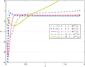
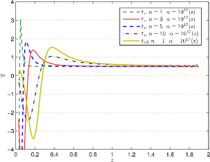
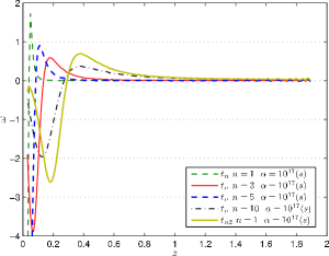
The effective deceleration parameter, as defined in (16), is plotted in Fig.16 for $t_{n1}$, used in our SFRW model. It shows the effective deceleration for different $n-$values. For $z\gg 1$ all models almost coincide and have $q=1/2$. They, however, differ from each other for small $z$. Negative deceleration is almost typical for all of them. Fig.18 shows the deceleration parameter for $t_{n}$.

4.4 Density contrast

Let us now look at the density contrast within the LTB domain. At any time, the density contrast within the LTB domain defined above is given by

$$\delta=\frac{\delta_{max}-\delta_{min}}{\delta_{min}}.$$ (26)

Calculation of $\delta$ is straightforward. We expect $\delta$ to be of the order of magnitude $10^{-5}$ for $z\approx 1100$ and of the order of magnitude 1 at the present time. Using $t_{n}$, there is a rather wide range of $\alpha$ and $n$ satisfying the density contrast conditions. Table 3 shows the density contrast for some of the parameter values.

$\alpha\,(\times 10^{17}s)$	$n$
$<0.5$	—	Not valid
$1$	$n\sim 1$	$\delta(z\approx 1100)\sim 10^{-7}$
$1$	$2<n<3$	Valid for both conditions
$1.5$	$1<n<4$	Valid for both conditions
$2$	$3<n<4$	Valid for both conditions
$3<\alpha<5$	$4<n<5$	Valid for both conditions

Table 3: Density contrast for $t_{n}$ and different parameter values.

The above results for $t_{n}$, and those of the luminosity distance ($\alpha=10^{17}~{}s$), shows that the inhomogeneity factor $n$ should be chosen in the range $1<n<3$. Note that the density contrast should not be greater than the desired order of magnitudes. In the opposite case, one can compensate the lack of contrast by adding some density perturbations as it is done in FRW models. In the case of $t_{n}$ for $\alpha=1$ the inhomogeneity factor $n$ has to be $<1$ to achieve the correct density contrast at the last scattering surface.

5 Conclusion

The Structured FRW model of the matter dominated universe we are proposing is a singularity free model which incorporates the concept of local inhomogeneities along the past light cone and is globally FRW. Although locally we have used the LTB metric, the effective model is a FRW type: along the light cone different Hubble parameters coincide, except for small values of z, as if we have just a FRW model. Therefore, we could consider this SFRW as a modified CDM/FRW with novel features. This is in contrast to familiar use of LTB metric to model local over- or under-dense bubbles. Not only the age of the universe is increased, the deceleration parameter has also an interesting behavior: it is negative for small $z$-values and goes to $1/2$ for larger redshifts. The density contrast changes from the order of magnitude $10^{-5}$ at the time of the last scattering surface to $1$ for the present time. Our model has two parameters $\alpha$ and $n$ both of the order of magnitude 1. The bang time is defined in a way that there is no central weak singularity present in the model; although it is not unique, the difference between different bang times in the class we have defined is marginal. We conclude that allowing for local changes along the past light cone one may construct model universes that behave Friedmanian but differs from the CDM model and leads to local acceleration, at the same time increases the age of the universe and reflects the growth of density contrast.

Figure 2: $t_{n}$ vs r using different functions. The blue curve for $t_{n}=\frac{\alpha}{r^{4}+r^{2}+1}$ and the red curve for $t_{n1}=\frac{\alpha}{r^{2}+1}$.

Figure 3: Light cone is shown (time vs $log_{10}(r)$) for $t_{n1}=\frac{\alpha}{r^{2}+1}\,\,,(\alpha=10^{17}s,n=1)$. The solid line curve shows the shell focussing area $R=0$ at $t=t_{n}$. On this curve both $R^{\prime}$ and $R^{\prime\prime}$ are singular. Here, one can easily see that one of these singular points lie on the light cone. This singular point maybe avoided if we restrict the value of n to be less than 0.2 or choose another bang time $t_{n}(r)$. The shell focussing singularity crosses the light cone at $z-$values well above the last scattering surface which is outside the range of applicability of our model, although it may also be avoided using suitable inhomogeneity parameter. The dash-dotted green curve corresponds to Kretschman singularity ($t=3t_{n}(r)$).

Figure 4: Similar to Fig.3, for $t_{n}=\frac{\alpha}{r^{4}+r^{2}+1}\,\,,(\alpha=10^{17}~{}s,n=1)$. All singularities are well inside the curve $t=3t_{n}(r)$. The $\dot{R^{\prime}}$ singularity points (corresponding to $t=t_{n}-\frac{1}{3}rt_{n}^{\prime}$) are not shown because they almost lie completely on the curve for $t=t_{n}(r)$.

Figure 5: $R^{\prime}$ is plotted versus $r$ for $t_{n}$ and different constant times. Looking at $R^{\prime}$ as an effective scale factor, it shows that the scale of the universe increases with time, although the rate of cosmic expansion is different at different places.

Figure 6: $\dot{R}^{\prime}$ vs $r$ for $t_{n}$ and $t=3\times 10^{17}~{}s$. No singularity is seen here.

Figure 7: A typical singular behavior of $R^{\prime}$ inside the light cone for $t_{n}$ and $t=8\times 10^{16}~{}s$. The bump after the singular point corresponds to the vanishing of $R^{\prime\prime}$.

Figure 8: A typical singular behavior of $\dot{R}^{\prime}$ vs $r$ for $t_{n}$ and constant $t=8\times 10^{16}~{}s$.

Figure 9: $t_{n}$, $R$, $r$ is drawn versus $z$. The bang time ($t_{n}$) is almost zero for $z>0.1$ . When we go back in time along the light cone, the scale of the universe (blue curve) goes to zero (i.e. $R\to 0$).

Figure 10: The SFRW effective scale factor $R/r$ as a function of $z$ for $t_{n}$ (blue curve). The red points show $R^{\prime}$ as a function of $z$. Both are almost the same for $z>0.1$. The effect of inhomogeneities is more clear for $z<0.1$ where $R^{\prime}\neq R/r$. The green curve shows the scale factor for a CDM/FRW model ($\alpha=0$).

Figure 11: Density $\rho$ as a function of $z$ for $t_{n}$ in low redshift region

Figure 12: Density $\rho$ as a function of $z$ for $t_{n}$ in high redshift region

Figure 13: Comparison of light cones for both SFRW (LTB) and FRW (CDM) models. The age of the Universe is greater in SFRW model by the factor $4/3$. We got these results for $z<1100$ (after last scattering time).

Figure 14: Using the luminosity distance and eq.15, the effective Hubble parameter is plotted. It shows also the Hubble parameter for CDM and $\Lambda$CDM models. Comparison of the effective Hubble parameter based on the luminosity distance ($H_{SFRW}$) and $\dot{R}^{\prime}/R^{\prime}$ shows, for all values of redshift parameter, these two definitions are the same. ($t_{n}=\frac{\alpha}{r^{4}+r^{2}+1},~{}n=1,~{}\alpha=10^{17}~{}s$)

Figure 15: $\mu=m-M$ vs $z$ (redshift) for different models (LCDM, CDM, $t_{n}$ SFRW).

Figure 16: The effective deceleration parameter for SFRW model ($t_{n1}=\frac{\alpha}{r^{2}+1}$) using the effective $H(z)$ and eq.16. This diagram clearly shows that, for small values of $z$, $q$ is negative and therefore, the universe is effectively accelerating at the present time. Increasing the parameter $n$, the transition of acceleration to deceleration occurs in higher redshifts.

Figure 17: The effective state parameter for SFRW model ($t_{n1}=\frac{\alpha}{r^{2}+1}$) using the effective $H(z)$ and eq.17.

Figure 18: Similar to Fig.16, using $t_{n}=\frac{\alpha}{r^{4}+r^{2}+1}$ and $t_{n2}=\frac{\alpha}{Ar^{4}+Br^{2}+1}$ for $A=0.0001,~{}B=0.001$.

Figure 19: Similar to Fig.17, using $t_{n}=\frac{\alpha}{r^{4}+r^{2}+1}$ and $t_{n2}=\frac{\alpha}{Ar^{4}+Br^{2}+1}$.