On what scale should inflationary observables be constrained?

Abstract

We examine the choice of scale at which constraints on inflationary observables are presented. We describe an implementation of the hierarchy of inflationary consistency equations which ensures that they remain enforced on different scales, and then seek to optimize the scale for presentation of constraints on marginalized inflationary parameters from WMAP3 data. For models with spectral index running, we find a strong variation of the constraints through the range of observational scales available, and optimize by finding the scale which decorrelates constraints on the spectral index $n_{{\rm S}}$ and the running. This scale is $k=0.017\,{\rm Mpc}^{-1}$, and gives a reduction by a factor of more than four in the allowed parameter area in the $n_{\rm S}$–$r$ plane ($r$ being the tensor-to-scalar ratio) relative to $k=0.002\,{\rm Mpc}^{-1}$. These optimized constraints are similar to those obtained in the no-running case. We also extend the analysis to a larger compilation of data, finding essentially the same conclusions.

I Introduction

In presenting observational constraints on the primordial power spectra, such as those that may have been generated by inflation, it is necessary to specify the scale at which the observables are being determined. Provided the full posterior distribution over all parameters is given, this choice is an arbitrary one. However, if the information is to be compressed via marginalization, the choice of this scale matters, and should be chosen in order to optimize the presentation of constraints.

In the Wilkinson Microwave Anisotropy Probe (WMAP) three-year cosmological parameters paper wmap3 the scale $0.002\,{\rm Mpc}^{-1}$ is used, which is close to the observable horizon, while Kurki-Suonio et al. KMV and Finelli et al. finelli found that the choice of $0.01\,{\rm Mpc}^{-1}$ worked better in constraining inflationary observables as it is closer to the statistical center of the data. The scale $0.05\,{\rm Mpc}^{-1}$ is also commonly used, being the default scale of the CosmoMC package CosmoMC . The pivot scale was also discussed in Ref. LLMP , who sought the scale where the perturbation amplitude was best determined (decorrelated with other power spectrum parameters), and in Ref. PE who sought the scale at which the perturbation spectrum reconstructed using the flow formalism was best constrained.

In this paper we make a systematic exploration of the choice of scale in the context of inflation models. This choice is particularly important in cases where models with significant spectral index running are allowed. Such models have received quite a bit of attention since the WMAP results emerged (see e.g. Refs. run ; EP ; KKMR ).

II Methodology

For definiteness we concentrate on single-field inflationary models, though many of the issues we discuss are more general. These models predict spectra of scalar and tensor perturbations which are related by a hierarchy of consistency equations LLKCBA ; CL , the first of which is, at lowest-order, the well-known relation $r=-8n_{{\rm T}}$ where $r$ is the tensor-to-scalar ratio and $n_{{\rm T}}$ the tensor spectral index. These parameters can in turn be related to the inflationary slow-roll parameters describing the shape of the potential.

Our main aim in this paper is to examine the optimal choice of scale at which to present observational constraints on inflation. In order to fit the spectra from data, they must first be parametrized, which is usually done by specifying their amplitude and some number of derivatives (i.e. the spectral index, running, etc) at a particular scale. So far, this scale has been chosen by hand.

The choice of scale, being arbitrary, ought not to affect the conclusions one draws. However this is only the case if one specifies the full multi-dimensional posterior parameter distributions, and provided the model definition is internally self-consistent. The first of these is often not the case, as one commonly wishes to condense information into one- or two-dimensional marginalized posterior distributions, which throws away the information on parameter correlations necessary to translate between scales. The second condition of model self-consistency holds in most circumstances, but often not in the way inflationary spectra are implemented.

The problem of model definition in inflationary models is the enforcement of the consistency equations between scalars and tensors. Typically both spectra are allowed to be power-laws but with different indices; if the usual consistency equation is enforced at one scale, it will then no longer hold at any other. Put another way, if the scalars are a perfect power-law, then the tensor spectrum implied by the consistency relations is not (unless the spectral indices are the same). Yet another way, the set of models generated by imposing the consistency equation at one scale is a different set of models from that obtained using another scale. This problem is further exacerbated if authors go on to include scalar spectral index running, while perhaps still leaving the tensors as a power-law. Before discussing the choice of scale, we should therefore first fix this problem (while admitting that the difference may be too small to be very important).

This is achieved by implementing the full inflationary consistency equation hierarchy, as given explicitly in Ref. CL . As well as the first consistency equation, this enforces that each derivative of the consistency equation also holds at a given scale. When using a Taylor expansion to shift from one scale to another, this hierarchy then ensures that the consistency equations will still hold at the new scale (up to some level set by the truncation of the hierarchy).

We note that these complications are needed only if one fits the phenomenological parameters (amplitude, spectral index, running, etc) from the data and then translates to inflationary observables. If instead one fits the slow-roll parameters directly (e.g. Ref. GL ; finelli ) or via flow equations flow ; KKMR ; PE then the consistency equation hierarchy is automatically enforced.

We consider a parametrization of the scalar and tensor perturbations as follows

$$A_{\rm S}^{2}(k) \propto (k/k_{*})^{(n_{\rm S}-1)+(dn_{\rm S}/d\ln k)\,\ln k/k_{*}}$$ (1)

$$A_{\rm T}^{2}(k) \propto (k/k_{*})^{n_{\rm T}+(dn_{\rm T}/d\ln k)\,\ln k/k_{*}}\,,$$ (2)

the constants of proportionality being the amplitude of the perturbations at scale $k_{*}$. The tensor-to-scalar ratio is defined by $r(k)\equiv 16A_{{\rm T}}^{2}(k)/A_{{\rm S}}^{2}(k)$, and the tensor spectral index is determined via the first consistency equation.

In order that the first consistency equation is enforced at all scales (to linear order in $\Delta\ln k$), we need to implement the second consistency equation to fix the tensor running, which is not a genuine new degree of freedom. This second equation is given by LLKCBA ; CL

$$\frac{dn_{\rm T}}{d\ln k}=n_{\rm T}\left[n_{\rm T}-(n_{\rm S}-1)\right]\,.$$ (3)

We enforce this when carrying out our data-fitting.

One could further enforce higher consistency equations, so that for instance the second consistency equation also is preserved under change of scales. However current data quality is a long way from the point where doing so would make any practical difference, since the tensors are potentially observable only over a limited range of scales.

We use the Monte Carlo Markov Chain (MCMC) technique to explore the parameter space, using the CosmoMC package CosmoMC . We consider a $\Lambda$CDM model in a flat universe and take $k_{*}=0.05\,{\rm Mpc}^{-1}$ as the scale where all power spectrum parameters are defined when fitting to data. We vary up to eight parameters

$$\Omega_{{\rm b}}h^{2},\Omega_{{\rm dm}}h^{2},\theta,\tau,n_{\rm S}(k_{*}),r(k_{*}),\ln[10^{10}A_{\rm S}(k_{*})],\left.\frac{dn_{\rm S}}{d\ln k}\right|_{k_{*}}$$

where $\Omega_{{\rm b}}h^{2}$ and $\Omega_{{\rm dm}}h^{2}$ are the physical baryon and dark matter densities, $\theta$ is the ratio of the sound horizon to the angular-diameter distance, $\tau$ is the optical depth, and the remaining parameters specify the power spectra. We apply a set of uniform priors:

$0.005<\Omega_{{\rm b}}h^{2}<0.1$	$0.01<\Omega_{{\rm dm}}h^{2}<0.99\,$
$0.5<\theta<10\,$	$0.01<\tau<0.8\,$
$0.5<n_{\rm S}<1.5\,$	$2.7<\log(10^{10}A_{\rm S})<4\,$
$0<r<2\,$	$-0.2<dn_{\rm S}/d\ln k<0.2\,$

Until Section V, our constraints are from WMAP3 data alone.

III Choice of scale: models with scalar running

We first consider models which allow running of the scalar spectral index, which we will see is the case where the choice of scale is most important. For comparison, models without running are studied in the next section.

III.1 Tilt and running

The simplest combination of observables to consider is the tilt and running of the scalars. Observational implications of this were first discussed in Ref. CGL , which forecasted CMB constraints from the Planck satellite on running spectral index models. The paper pointed out that there would be a scale at which the uncertainties on tilt and running would become uncorrelated, and that (at least in a gaussian approximation) on that scale the uncertainty in $n$ would recover its value for the case of no running. This could be spoiled by degeneracies with other parameters, but at Planck accuracy appears not to be CGL .

Anyway, we wish to find the scale at which the tilt and running decorrelate for actual current data. To do this we take the distribution of these two variables as given by the MCMC analysis, which specifies quantities at $k_{*}=0.05\,{\rm Mpc}^{-1}$. We then fit the chain elements with a linear relation, $n_{\rm S}=A+B\,dn_{\rm S}/d\ln k$, and by inserting into the expression

$$n_{\rm S}(k)=n_{\rm S}(k_{*})+\frac{dn_{\rm S}}{d\ln k}\ln\frac{k}{k_{*}}\,,$$ (4)

we arrive at a condition for the difference in scale which decorrelates $n_{\rm S}$ and $dn_{\rm S}/d\ln k$: $B=-\ln k/k_{*}$. This scale turns out to be $k=0.017\,{\rm Mpc}^{-1}$. Then we use Eq. (4) to convert the distribution at scale $k_{*}$ to the one at scale $k=0.017\,{\rm Mpc}^{-1}$ to obtain the decorrelated $n_{\rm S}$ and $dn_{\rm S}/d\ln k$. More generally, we can explore the constraints at other scales via the same formalism. The constraints at a set of different scales, including the WMAP scale and the decorrelation scale, are shown in Fig. 1.

Figure 1: Constraints in the $n_{\rm S}$–$\alpha$ plane (where $\alpha=dn_{\rm S}/d\ln k$) at several scales. $k=0.017\,{\rm Mpc}^{-1}$ is the decorrelation scale for these parameters.

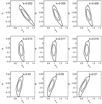
In this particular case (but not those that follow), the transformation between parameters induced by the scale change has unit Jacobian, which means that the 2D contour areas are preserved. However it is clear from Fig. 1 that the marginalized uncertainty on $n_{{\rm S}}$ at the decorrelation scale is significantly smaller. The WMAP choice, $0.002\,{\rm Mpc}^{-1}$, gives a significantly-angled constraint area and is clearly to be avoided if useful marginalized constraints on $n_{{\rm S}}$ are to be quoted. Unfortunately, the main WMAP3 results for models with running are presented at this scale.

For our choice of parameters and dataset (WMAP3 alone), from separate fits where running is not included we find the marginalized constraint on $n_{\rm S}$ is $n_{\rm S}=0.993_{-0.030,-0.053}^{+0.029,+0.067}$ (at 68% and 95% confidence). With running, the marginalized constraint at the decorrelation scale is $n_{\rm S}=0.981_{-0.034,-0.063}^{+0.034,+0.067}$. As anticipated, therefore, when including running the shift in the best-fit $n_{\rm S}$ at the optimized scale is negligible within the uncertainty. This is somewhat trivial as it could have been chosen to match exactly by specific choice of scale — choosing $k=0.015\,{\rm Mpc}^{-1}$ achieves this. Much more importantly, we see that the uncertainty on $n_{{\rm S}}$ at the decorrelation scale is hardly increased when running is included, whereas it is greatly increased at e.g. $0.002\,{\rm Mpc}^{-1}$. The 1D marginalized constraints on all parameters have minimum uncertainty at the decorrelation scale.

Incidentally, for the scalar running the marginalized constraints we obtained are $dn_{\rm S}/d\ln k=-0.075_{-0.043,-0.093}^{+0.041,+0.082}$, very similar to those quoted by WMAP3 for models with running and tensors wmap3 .

III.2 Tilt and the tensor–scalar ratio

We now turn to other combinations of observables, relevant to constraining inflation.

To obtain $r$ at other scales we perform an expansion, to the order considered, of the scalar and tensor amplitudes. The relation is

$$\frac{r(k)}{r(k_{*})}=\frac{1+n_{\rm T}\ln\frac{k}{k_{*}}+\frac{1}{2}\left[n_{\rm T}^{2}+\frac{dn_{\rm T}}{d\ln k}\right]\ln^{2}\frac{k}{k_{*}}}{1+(n_{\rm S}-1)\ln\frac{k}{k_{*}}+\frac{1}{2}\left[(n_{\rm S}-1)^{2}+\frac{dn_{\rm S}}{d\ln k}\right]\ln^{2}\frac{k}{k_{*}}}\,.$$ (5)

where all observables without an argument ‘(k)’ are evaluated at $k_{*}=0.05\,{\rm Mpc}^{-1}$, and where $dn_{\rm T}/d\ln k$ was set according to the lowest-order version of the second consistency equation, Eq. (3). Having expressions for $n_{\rm S}$ and $r$ at different scales, we can now choose several scales and get the distribution of the two variables at each, shown in Fig. 2.

Figure 2: Constraints on $n_{\rm S}$ versus $r$ at several scales.

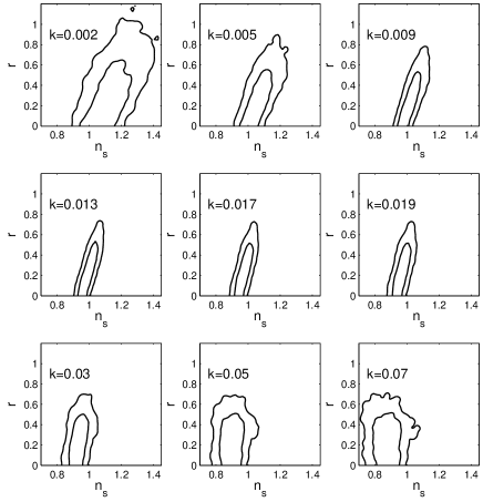
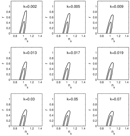
In this case the transformation alters the contour areas as well as distorting them. The middle panel of Fig. 3 shows the areas enclosed by the 95% confidence contour in the $n_{\rm S}$–$r$ plane at different scales. The top panel shows the same for $n_{\rm S}$ and running discussed in the previous subsection. In the $n_{\rm S}$–$r$ plane the minimum area was near $k=0.017\,{\rm Mpc}^{-1}$ as expected (the precise value found was slightly smaller). As inflation model builders typically just look at these marginalized plots to decide if their model is viable, it is clearly important to present the constraints at a good scale. $0.002\,{\rm Mpc}^{-1}$ is not a good scale for this purpose, as has previously been stressed also in Ref. PE .

Figure 3: Variation of parameter plane area with scale. For the $\epsilon$–$\eta$ case both lowest (black, full) and next order (red, dashed) are shown. For $n_{\rm S}$ versus running the area should be independent of scale, and the variations indicate the noise level in the area estimation.

III.3 Inflationary slow-roll parameters: lowest order

We now examine how the constraints on the first two slow-roll parameters $\epsilon$ and $\eta$ are affected by scale change. We take the usual definitions in terms of the potential LL92

$$\epsilon=\frac{m_{{\rm Pl}}^{2}}{16\pi}\left(\frac{V^{\prime}}{V}\right)^{2}\quad;\quad\eta=\frac{m_{{\rm Pl}}^{2}}{8\pi}\,\frac{V^{\prime\prime}}{V}\,.$$ (6)

The pivot scale $k_{*}$ corresponds to some particular scalar field value $\phi_{*}$ (defined as the field value when $k_{*}=aH$ during inflation), in the vicinity of which the scalar field potential is being reconstructed. Shifting the pivot scale means expanding about a different point on the potential.

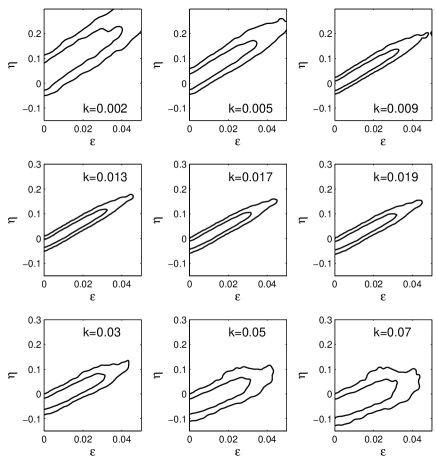
We first concentrate on the constraints given at lowest order, taking the expressions for the potential at this order by Lidsey et al. LLKCBA :

$$V(\phi) \simeq \frac{75m_{\rm Pl}^{4}}{32}A_{\rm T}^{2}(k)\,,$$

$$V^{\prime}(\phi) \simeq -\frac{75\sqrt{\pi}}{8}m_{\rm Pl}^{3}\frac{A_{\rm T}^{3}(k)}{A_{\rm S}(k)}\,,$$ (7)

$$V^{\prime\prime}(\phi) \simeq \frac{25\pi}{4}m_{\rm Pl}^{2}A_{\rm T}^{2}(k)\left[9\frac{A_{\rm T}^{2}(k)}{A_{\rm S}^{2}(k)}-\frac{3}{2}[1-n_{\rm S}(k)]\right]\,,$$

(where without loss of generality we take $\phi$ to increase in time). From these the first two slow-roll parameters are expressed in terms of the observables, to lowest order, by

$$\epsilon\simeq\frac{r}{16}\quad;\quad\eta\simeq\frac{3}{16}r-\frac{1}{2}(1-n_{\rm S})\,.$$ (8)

Shifting the scale of the observables shifts the location on the potential, and at lowest-order the constraints on $\epsilon$ and $\eta$ then become independent of the running at that scale (which could be used to determine a third slow-roll parameter $\xi\equiv m_{{\rm Pl}}^{2}/8\pi\sqrt{V^{\prime}V^{\prime\prime\prime}/V^{2}}$).

Figure 4: Constraints on $\epsilon$ versus $\eta$, at lowest order, evaluated at several scales.

The results are presented in Fig 4, and again show strong variation of the allowed parameter area with choice of scale, as indicated in Fig. 3.

III.4 Inflationary slow-roll parameters: next order

Now we can take the expressions for the potential to next order SL , also given by Lidsey et al. LLKCBA :

$$V(\phi) \simeq \frac{75m_{\rm Pl}^{4}}{32}A_{\rm T}^{2}\left[1+\left(\frac{5}{3}+2C\right)\frac{A_{\rm T}^{2}}{A_{\rm S}^{2}}\right]\,,$$

$$V^{\prime}(\phi) \simeq -\frac{75\sqrt{\pi}}{8}m_{\rm Pl}^{3}\frac{A_{\rm T}^{3}}{A_{\rm S}}\left[1-0.85\frac{A_{\rm T}^{2}}{A_{\rm S}^{2}}+0.53(1-n_{\rm S})\right]\,,$$

$$V^{\prime\prime}(\phi) \simeq \frac{25\pi}{4}m_{\rm Pl}^{2}A_{\rm T}^{2}\Big{\{}9\frac{A_{\rm T}^{2}}{A_{\rm S}^{2}}-\frac{3}{2}(1-n_{\rm S})$$

$$+\Big{[}(36C+2)\frac{A_{\rm T}^{4}}{A_{\rm S}^{4}}-\frac{1}{4}(1-n_{\rm S})^{2}-$$

$$\quad(12C-6)\frac{A_{\rm T}^{2}}{A_{\rm S}^{2}}(1-n_{\rm S})-\frac{1}{2}(3C-1)\frac{dn_{\rm S}}{d\ln k}\Big{]}\Big{\}}\,,$$

where $C=-2+\ln 2+\gamma\simeq-0.73$, $\gamma$ is the Euler–Mascheroni constant, and again the $\phi$ value corresponds to horizon crossing of the scale at which the constraints are being imposed.

Figure 5: Constraints on $\epsilon$ versus $\eta$, to next order, at several scales.

With these next-order expressions for the potential, $\epsilon$ and $\eta$ are

$$\epsilon = \frac{r}{16}\,\frac{1-0.85\,r/16+0.53(1-n_{\rm S})}{1+0.21\,r/16}$$ (10)

$$\eta = \frac{1}{3}\frac{1}{1+0.21\,r/16}\Big{\{}\frac{9}{16}r-\frac{3}{2}(1-n_{\rm S})$$

$$+(36C+2)\left(\frac{r}{16}\right)^{2}-\frac{1}{4}(1-n_{\rm S})^{2}$$

$$-(12C-6)\frac{r}{16}(1-n_{\rm S})-\frac{1}{2}(3C-1)\frac{dn_{\rm S}}{d\ln k}\Big{\}}\,.$$

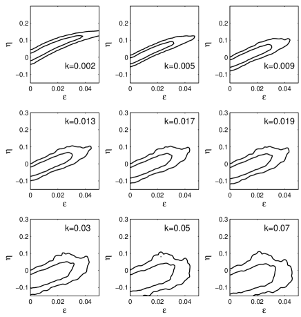
The second parameter now depends on the running. The running term has a coefficient of about one half, and given how weakly running is constrained this term has a significant impact on the constraints.

The constraints at each scale are presented in Fig 5. The picture here is rather different, with the area changing much more slowly as $k$ is decreased, and the minimum area being at a much smaller $k$. This is because for typical models the next-order correction from the running happens to be comparable to the change in the lowest-order expression for $\eta$ coming from the changing $n_{{\rm S}}$, also induced by the running, as the scale changes. These terms approximately cancel going to smaller $k$, i.e. the constraints change less when simultaneously reducing $k$ and introducing next-order corrections than they would if only one of these were done. This is just a coincidence (and not much of a coincidence at that, since partial cancellation would have to happen as $k$ was changed in one or other direction) of no great significance, and will go away when in future running is better constrained.

Figure 6: Constraints on $n_{\rm S}$ and $r$ when no scalar running is present.

IV Choice of scale: models with no scalar running

For comparison, we now take a look at models where no running of the scalar index is allowed. In this case the variation in the constraints with scale is much less, as for instance is seen in Fig. 6 showing the $n_{\rm S}$–$r$ plane. Indeed in this case we find that minimization of the area is not only unnecessary, but can actually be misleading, because parameters such as $r$ can appear to be well constrained even on scales where there is no meaningful data. The reason for this is that the restrictive class of models under consideration force the spectra to behave in a particular way as they are extrapolated away from the region where the bulk of the data lie, i.e. such constraints contain significant prior information as well as data information. This is also true to some extent for constraints on $r$ in the running case studied earlier.

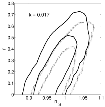
Nevertheless, it is now interesting to compare the running and no-running constraints. In the WMAP3 analysis the impression, from comparison of the top-left panels of Figs. 12 and 14 of Ref. wmap3 , is of a huge deterioration in the constraints in the $n_{\rm S}$–$r$ plane once running is included. The same is seen in Fig. 1 of Ref. KKMR . However we now see that this is an artifact of the choice of scale where the constraints are portrayed. At the optimal scale there is some deterioration, due to parameter degeneracy, but the area increase within the 95% contour is only by about 20% as seen in Fig. 7, not by a factor of five as at $k=0.002\,{\rm Mpc}^{-1}$. Consequently, inclusion of running leads only to a moderate deterioration in constraints on $\epsilon$ and $\eta$.

Figure 7: Comparison of constraints in the $n_{\rm S}$–$r$ plane at the optimal scale with no running (dotted contours) and when running is included (full contours). The area enclosed by the 95% contour increases by around 20% when running is included.

V Including more data

We explore the robustness of our results by carrying out the same analysis for a broader compilation of data, now including shorter-scale CMB experiments and galaxy correlation data from ACBAR ACBAR , CBI CBI , VSA VSA , Boomerang boom , SDSS SDSS , and 2dFGRS 2df .

Everything goes through as before. We find that the decorrelation scale of $n_{\rm S}$ and running is $0.016\,{\rm Mpc}^{-1}$, which is not significantly different from WMAP3 alone. Though in general one would expect the decorrelation scale to change with dataset, in this case the WMAP3 data are powerful enough that a shift is not seen.

Figure 8: As Fig. 4, but now with the full dataset compilation. Note the modified axis ranges.

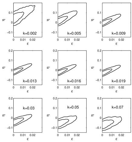
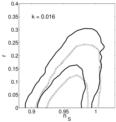
The constraints, particularly on $r$ and hence $\epsilon$, do tighten significantly with the extra data, as is clear also in previous analyses including Ref. wmap3 . As an illustration of the results we obtained in this case, we show the array of constraints on the lowest-order $\epsilon$ and $\eta$ at different scales, Fig. 8, and the overlay of contours in the $n_{\rm S}$–$r$ plane at the optimal scale, with and without running, in Fig. 9.

Figure 9: As Fig. 7, but now with the full dataset compilation. Note the modified axis ranges. The area enclosed by the 95% contour increases by around 30% when running is included.

VI Conclusions

We have investigated the issue of choice of scale in presenting marginalized parameter constraints. While we have focussed on WMAP constraints applied to inflationary models, the same considerations apply much more widely. For example, in constraining density perturbations using galaxy clusters, commonly the parameter $\sigma_{8}$, being the normalization of density perturbations smoothed on the scale $8h^{-1}\,{\rm Mpc}^{-1}$, is quoted. However typically the normalization is best determined at a somewhat larger scale than $8h^{-1}\,{\rm Mpc}$, and marginalizing over parameters such as $\Omega_{0}$ to quote constraints on $\sigma_{8}$ can unnecessarily increase the statistical uncertainty on the normalization.

In the inflationary context, choosing an optimal scale is important primarily in models where large running is allowed. We found that an appropriate scale is the one which decorrelates estimates of $n_{\rm S}$ and running, which for WMAP3 is $0.017\,{\rm Mpc}^{-1}$. This criterion can be used to define such a scale for any dataset compilation, and we found that the scale shifts hardly at all when other available data are added to WMAP3. The optimal scale may also have some modest dependence on the choice of model parameters varied in a fit, for instance if non-negligible neutrino masses were included. One might even wonder whether it might be best to choose different scales for different observables, as the scalars and tensors are best constrained on quite different length scales, but we have not attempted this here.

We have shown that the marginalized constraints on $n_{\rm S}$ and $r$, or on $\epsilon$ and $\eta$, depend significantly on the choice of scale in the presence of running. By choosing the optimal scale, we find that constraints on those parameters are only mildly degraded by the inclusion of running as a parameter, in contrast to the impression given if constraints are quoted at a non-optimal scale such as $0.002\,{\rm Mpc}^{-1}$.