A Scaling Index Analysis of the WMAP three year data: Signatures of non-Gaussianities and Asymmetries in the CMB

Abstract

Local scaling properties of the co-added foreground-cleaned three-year Wilkinson Microwave Anisotropy Probe (WMAP) data are estimated using weighted scaling indices $\alpha$. The scaling index method (SIM) is - for the first time - adapted and applied to the case of spherical symmetric spatial data. The results are compared with $1000$ Monte Carlo simulations based on Gaussian fluctuations with a best fit $\Lambda$CDM power spectrum and WMAP-like beam and noise properties. Statistical quantities based on the scaling indices, namely the moments of the distribution and probability-based measures are determined. We find for most of the test statistics significant deviations from the Gaussian hypothesis. Using a very conservative $\chi^{2}$ statistics, which averages over all scales, we detect non-Gaussianity with a probability of $97.3$ % regarding the Kp0-masked full sky, $98.9$ % for the Kp0-masked northern and $91.6$ % for the Kp0-masked southern hemisphere. When analysing different length scales separately, the detection rates increase to $99.7$ % ($>99.9$ % north, $97.4$ % south) for the mean, $98.4$ % ($99.9$ % north, $71.6$ % south) for the standard deviation and $97.9$ % ($99.4$ % north, $80.3$ % south) for a $\chi^{2}$-combination of mean and standard deviation. We find pronounced asymmetries, which can be interpreted as a global lack of structure in the northern hemisphere, which is consistent with previous findings. Furthermore, we detect a localized anomaly in the southern hemisphere, which gives rise to highly significant signature for non-Gaussianity in the spectrum of scaling indices $P(\alpha)$. We identify this signature as the cold spot, which was also already detected in the first year WMAP data. Our results provide further evidence for both the presence of non-Gaussianities and asymmetries in the WMAP three-year data. More detailed band- and year-wise analyses are needed to elucidate the origin of the detected anomalies. In either case the scaling indices provide powerful nonlinear statistics to analyse CMB maps.

1 Introduction

The study of the Gaussianity of the Cosmic Microwave Background (CMB) is regarded to be the best way for understanding the true nature of the primordial density fluctuations: by measuring suitable statistics of the temperature fluctuations of the CMB and comparing the results with theoretical predictions, cosmological models for the primordial density fluctuations can be rejected or accepted at a certain confidence level. Standard inflationary models (Guth, 1981; Linde, 1982; Albrecht & Steinhard, 1982) predict that the temperature fluctuations of the CMB correspond to a (nearly) Gaussian, homogeneous and isotropic random field. In fact, Gaussianity and statistical isotropy are among the fundamental pillars of the $\Lambda$CDM concordance cosmological model. On the other hand, many alternative scenarios have been studied, which give rise to non-Gaussianity, e.g. non-standard inflation (Linde & Mukhanov, 1997; Peebles, 1997; Bernardeau & Uzan, 2002; Acquaviva et al., 2003), or topological defects models (Bouchet, Bennett, & Stebbins, 1988; Turok, & Spergel, 1990; Turok, 1996) to mention a few. Probing non-Gaussianity therefore represent one of the key tests to detect deviations from the minimal scenario. To detect them it is essential to have high sensitivity and large-coverage CMB data.
The Wilkinson Microwave Anisotropy Probe (WMAP) satellite has produced high resolution all-sky observations of the CMB with unprecendented accuracy, which have confirmed many predictions of the $\Lambda$CDM concordance cosmological model (Spergel et al., 2003; Bennett et al., 2003; Spergel et al., 2006).
First analyses based on the WMAP first year data and global statistical measures did not show significant deviations from the Gaussianity hypothesis (Komatsu et al., 2003). A number of subsequent studies of the first-year WMAP-data yielded, however, evidence for non-Gaussian features as well as asymmetries in the CMB as measured with the WMAP data.
These results were obtained using a number of qualitatively different statistical tests ranging from (local) spectral (de Oliveira-Costa et al., 2004; Copi et al., 2004; Eriksen et al., 2004b; Hansen, Banday, & Górski, 2004; Land, 2005) and $N$-point correlation function analysis (Eriksen et al., 2004b, 2005a), to Fourier phases (Chiang et al., 2003; Coles et al., 2004; Naselsky et al., 2005), Minkowski - functionals (Park, 2004; Eriksen et al., 2004a) and wavelets (Vielva et al., 2004; Cruz et al., 2005; McEwen et al., 2005).
In March 2006 the three-year WMAP results were released and several groups revisited the anomalies found in the first data release. Considering the fact that the first year WMAP data were already of very high quality it was no surprise that many of the anomalies found in the first year data were redetected (Bridges et al., 2006; Copi et al., 2006; Jaffe et al., 2006; Land, 2006; Martínez-González et al., 2006) in the three year data release albeit none of these tests alone showed outstanding significance. Hence there is an ongoing discussion, whether the identified features are significant enough to prove asymmetry or non-Gaussianity of the CMB. Given the tremendous consequences a claim of non-Gaussianity of the CMB on cosmology would have, some caution in making such statements is warranted.
Non-Gaussianity cannot be defined in a unique manner, it is simply the presence of any higher order spatial correlations. Therefore, there cannot be one unique test for all possible ways a random field can be non-Gaussian that is preferable to other tests, or that has superior sensitivity. In order to perform a thorough analysis, one rather has to apply several different, preferably complementary tests. Following this reasoning, we present in this paper a novel approach to analyse observed CMB-data on a local scale and to test for Gaussianity and (statistical) isotropy. Namely we estimate the local scaling properties of the maps of temperature fluctuations using weighted scaling indices (see e.g. Räth et al. (2002); Räth & Schuecker (2003)). These scaling indices are sensitive to the local morphological properties of the field of the temperature fluctuations $\Delta T(\theta,\phi)$ at a given scale $r$. It has been demonstrated that this statistic is highly sensitive to non-Gaussian signatures in simulated CMB-maps. Here, we propose a formalism that can be applied to observed WMAP-data with its spherical symmetry and test for both non-Gaussianties and statistical asymmetries in the WMAP three-year data using Monte Carlo simulations based on Gaussian fluctuations with a best fit $\Lambda$CDM power spectrum and WMAP-like beam and noise properties.
The paper is organised as follows. In Section 2 we describe the WMAP-data as well as the simulations and the preprocessing steps, which were applied to both the simulated and observed data. In Section 3 we review the formalism of the weighted scaling indices and explain it with a simple example. As the weighted scaling indices and the wavelets share some properties (e.g. locality, scale dependence) we compare the two test statistics, show similarities and outline differences. We further extend the scaling index formalism to the application to spherical WMAP-data. In Section 4 the results of the WMAP three-year data analysis are presented. We summarize our main results in Section 5 and present our conclusions in Section 6.

2 WMAP Data, Simulations and Preprocessing

We use the noise-weighted sum $T$ of the V1, V2, W1, W2, W3 and W4 foreground-cleaned maps,

$$T(\theta,\phi)=\frac{\sum_{j=5}^{10}T_{j}(\theta,\phi)/\sigma^{2}_{0,j}}{\sum_{j=5}^{10}1/\sigma^{2}_{0,j}}$$ (1)

where $j=5,6$ refer to the two V-band receivers and $j=7,\ldots,10$ to the four W-bands. $\sigma^{2}_{0,j}$ denotes the three-year noise per observation for the six frequency bands given by Hinshaw et al. (2006). In contrast to many of the one-year Gaussianity studies (e.g. Komatsu et al. (2003); Vielva et al. (2004)) the Q bands were no longer taken into account, because they exhibit foreground contaminations. All these foreground cleaned maps were taken from the publicly accessible LAMBDA website.
In order to study the Gaussianity of the coadded VW-WMAP maps, we generated and analysed a set of 1000 Gaussian Monte Carlo simulations. For this we took the set of the best fit $C_{l}$’s (WMAP only) as published on the LAMBDA-site some weeks after the three year data release . For the set of $C_{l}$’s, random $a_{lm}$’s for the $C_{l}$’s of CMB realizations were generated and convolved at each one of the WMAP receivers with the appropriate beam transfer functions . After the transformation from harmonic to real space, uncorrelated Gaussian noise realizations were added following the number of observations per pixel $N_{j}(\theta,\phi)$ and the noise dispersion per observation ($\sigma_{0j}$). We combined all the maps following equation (1). Finally, both the coadded WMAP-data and the simulations were degraded to $N_{side}=256$, the Kp0 mask was applied, and the residual monopole and dipoles were fitted and subtracted. All these simulation and preprocessing steps were performed with the HEALPIX-software (Górski et al., 2005).

3 Weighted Scaling Indices

The weighted scaling index method (SIM) (Räth et al., 2002; Räth & Schuecker, 2003) offers one possibility to estimate the local scaling properties of a set of points, which is generally repesented in a $d-$dimensional space. The SIM has found applications in (astrophysical) time series analysis of AGNs, where the observed light curves were represented as point distributions by embedding the time series in a higher dimensional artificial phase space using delay coordinates (Gliozzi, et al., 2002; Gliozzi, Papadakis, & Räth, 2006).
Scaling indices have also often successfully been used for structure analysis in 2D and 3D image data (Jamitzky et al., 2001; Monetti et al., 2003; Mueller et al., 2004). For this the image data are represented as point distributions by comprising the spatial and intensity information of each pixel. For two-dimensional images one thus obtains a set of three-dimensional vectors $\vec{p_{i}}=(x_{i},y_{i},I(x_{i},y_{i}))$,$i=1,\ldots,N_{pixels}$. On the basis of the representation of images as point distributions the weighted scaling indices are calculated as follows:

3.1 General Formalism

Consider a set of $N$ points $P=\{\vec{p_{i}}\},i=1,\ldots,N$. For each point the local weighted cumulative point distribution $\rho$ is calculated. In general form this can be written as

$$\rho(\vec{p_{i}},r)=\sum_{j=1}^{N}s_{r}(d(\vec{p_{i}},\vec{p_{j}}))\;,$$ (2)

where $s_{r}(\bullet)$ denotes a kernel function depending on the scale parameter $r$ and $d(\bullet)$ a distance measure.
The weighted scaling indices $\alpha(\vec{p_{i}},r)$ are obtained by calculating the logarithmic derivative of $\rho(\vec{p_{i}},r)$ with respect to $r$,

$$\alpha(\vec{p_{i}},r)=\frac{\partial\log\rho(\vec{p_{i}},r)}{\partial\log r}=\frac{r}{\rho}\frac{\partial}{\partial r}\rho(\vec{p_{i}},r)\;.$$ (3)

In principle, any differentiable kernel function and any distance measure can be used for calculating $\alpha$. In the following we use the euclidean norm as distance measure and a set of gaussian shaping functions. So the expression for $\rho$ simplifies to

$$\rho(\vec{p_{i}},r)=\sum_{j=1}^{N}e^{-(\frac{d_{ij}}{r})^{q}}\;,d_{ij}=\|\vec{p_{i}}-\vec{p_{j}}\|\;.$$ (4)

The exponent $q$ controls the weighting of the points according to their distance to the point for which $\alpha$ is calculated. The higher $q$ is the more steplike becomes the weighting function resembling more and more the Heaviside-function, which is used for the calculation of the unweighted scaling indices. Another interesting choice of $q$ is given by $q=2$. In this case the kernel function is the well-known Gaussian exponential function.
Throughout this study we calculate $\alpha$ for the case $q=2$. Inserting the expression (4) in the definition for the weighted scaling indices in (3) yields after some algebra the following analytical expression for $\alpha$:

$$\alpha(\vec{p_{i}},r)=\frac{\sum_{j=1}^{N}q(\frac{d_{ij}}{r})^{q}e^{-(\frac{d_{ij}}{r})^{q}}}{\sum_{j=1}^{N}e^{-(\frac{d_{ij}}{r})^{q}}}\;.$$ (5)

Structural components of a point set are characterized by the calculated value of $\alpha$. For example, points in a point-like structure have $\alpha\approx 0$ and pixels forming line-like structures have $\alpha\approx 1$. Area-like structures are characterized by $\alpha\approx 2$ of the pixels belonging to them. A uniform distribution of points yields $\alpha\approx d$ which is equal to the dimension of the configuration space. The scaling indices for the point set form the frequency distribution $N(\alpha)$

$$N(\alpha)d\alpha=\#(\alpha\in[\alpha,\alpha+d\alpha[)$$ (6)

or equivalently the probability distribution

$$P(\alpha)d\alpha=Prob(\alpha\in[\alpha,\alpha+d\alpha[)$$ (7)

The $P(\alpha)$-representation of a point set can be regarded as a structural decomposition of the data where the points are differentiated according to the local morphological features of the structure elements to which they belong to.

3.2 Scaling Indices and Wavelets

Some test statistics, with which non-Gaussian signatures have been detected in the first and three-year WMAP-data, are based on a wavelet analysis of the CMB data, e.g. (Vielva et al., 2004; McEwen et al., 2005). Beside the fact that wavelet-based tests yield one of the highest significances for non-Gaussianities in the WMAP-data, wavelets and scaling indices can also be considered to be similar to each other. Both measures perform a local analysis of e.g. image data and they are calculated for different scales, which yields information about characteristic sizes of detected features. On the other hand, there are obvious differences. While the scaling indices are a nonlinear and non-bijective local filter, the wavelet transformation is a linear operation, namely a scale- and space-dependent filtering of the image data with a wavelet function $\Psi$:

$$w(b_{x},b_{y},r)=\int{dxdyI(x,y)\Psi(x,y;b_{x},b_{y},r)}$$ (8)

For the special case of spherical mexican hat wavelets (SMHW), the ’mother wavelet’ $\psi(d,r)$ is defined by:

$$\Psi(d,r) \equiv \Psi(d,b_{x}=0,b_{y}=0,r)$$ (9)

$$= \frac{1}{(2\pi)^{1/2}r}\left[2-\left(\frac{d}{r}\right)^{2}\right]e^{-d^{2}/2r^{2}}$$

with $d=\sqrt{x^{2}+y^{2}}$. It has been shown (Martínez-González et al., 2002) that SMHW yield superior results in detecting non-Gaussian signatures compared to other filter functions, e.g. Haar wavelets.
To consider the performance of the scaling indices in the context of known test statistics for non-Gaussianities we calculate and compare scaling indices and SMHW for two examples.
In the first simple example we generated a synthetic image which consists of a (white Gaussian) noisy background, where the noise level was chosen to be twice as high in the lower third of the image than in the rest of the image. We interspersed three single-coloured lines and six disc-like elements in the noisy background. The intensities of the structural elements ranged from $0\sigma$ to $\pm 1\sigma$ with respect to the standard deviations of the different noisy backgrounds (see Figure 1).

Figure 1: Left to right: Synthetic test image, response image of the scaling indices and response image of the wavelet coefficients. The response images were normalised to the range of values of the scaling indices and wavelets respectively.

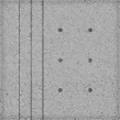
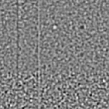
We calculated the wavelets and scaling indices for a corresponding and well-suited scale. Figure 1 shows the grey-value coded response of the wavelet and scaling index filter. One can see that the wavelets can only detect those discs, which deviate most from the mean value of the noise. The lines are only hardly detected in the less noisy background. The scaling indices, however, can detect all interspresed structural elements in the image, where the (inner part of the) disc-like structures have lower $\alpha$-values than the three lines. The observed differences in the images of the filter response find their reflections in the probability distributions $P(\alpha)$ and $P(w)$ for the scaling indices and wavelet coefficients (Figure 2).

Figure 2: Probability distribution of the the scaling indices (above) and wavelet coefficients (below). The gray lines indicate the distributions for the pure noise image without the line- and disc-like structural elements.

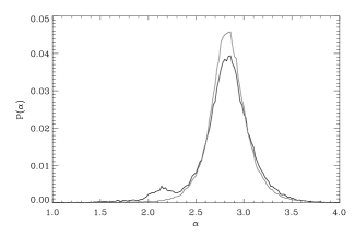
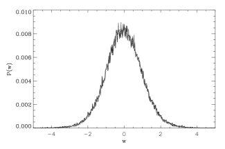
While the spectrum of scaling indices shows a clear second peak at $\alpha\approx 2.1$ and a larger tail towards lower $\alpha$-values, no visible deviations can be seen in the in the distribution of the wavelet coefficients when compared with those for a pure noisy image. With this example it becomes obvious that the wavelets are more sensitive to structures, which are associated with intensity variations of significant magnitude with respect to image noise. The scaling indices can, however, detect also structural features, which do not manifest themselves with significantly higher (lower) intensity values but as intrinsic structural variations within the noise level.
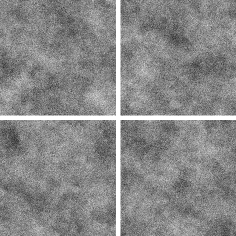
In the second more realistic example we consider a realisation of CMB anisotropies due to the Kayser-Stebbin effect from cosmic strings on which white additive Gaussian noise was superimposed. The noise level is chosen with rms signal-to-noise-ratio (S/N) of 0.5. For this image 20 surrogate maps were generated, which have the same power spectrum and amplitude distribution as the original simulation (Figure 3).

Figure 3: Simulated non-Gaussian CMB map with superimposed white additive noise (lower left) and three surrogate realisations with the same power spectrum and amplitude distribution.

Figure 4: Significances of the moments of the distribution of scaling indices (black) and wavelet coefficients (gray) for the image in fig. 3. The lines and $+$ denote the mean, the dotteds line and $\star$ the standard deviation, dashed lines the skewness and dashdotted lines and $\diamond$ the kurtosis.

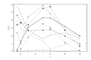
For more details about the simulation and its surrogates see Räth & Schuecker (2003). We compare tests for non-Gaussianities based on wavelets and scaling indices. In both cases we use the moments of the distributions of wavelet coefficient and scaling indices as test statistics, namely the mean ($<\alpha>$), standard deviation ($\sigma_{\alpha}$), skewness ($\gamma_{\alpha}$) and kurtosis ($\kappa_{\alpha}$), which are defined by

$$<\alpha>=\frac{1}{N}\sum_{i=1}^{N}\alpha_{i}$$ (10)

$$\sigma_{\alpha}=\left(\frac{1}{N-1}\sum_{i=1}^{N}(\alpha_{i}-<\alpha>)^{2}\right)^{1/2}$$ (11)

$$\gamma_{\alpha}=\frac{1}{N}\sum_{i=1}^{N}\left(\frac{(\alpha_{i}-<\alpha>)}{\sigma_{\alpha}}\right)^{3}$$ (12)

$$\kappa_{\alpha}=\frac{1}{N}\sum_{i=1}^{N}\left(\frac{(\alpha_{i}-<\alpha>)}{\sigma_{\alpha}}\right)^{4}-3$$ (13)

as test statistics. For each statistic the degree of detected non-Gaussianity is measures in terms of significance $S$,

$$S=\left|\frac{M-<M>}{\sigma_{M}}\right|$$ (14)

where $M$ is $<\alpha>,\sigma_{\alpha},\gamma_{\alpha}$ and $\kappa_{\alpha}$ respectively. The mean and standard deviation of the measure $M$ are derived from the 20 surrogate reliasations. Figure 4 summarizes the results for the scaling indices and SMHW. Both classes of filters can well detect the non-Gaussianities even at this high noise level. The highest significances occur at similar scales. However, the best results were obtained for different moments. While for the scaling indices the standard devaition performed best, we found for the wavelets the best discrimination with the kurtosis. The second best result for the scaling indices was obtained with the mean. Based on these findings we restrict ourselves to the analysis of the mean and standard deviation of the distribution of scaling indices for the WMAP data. In summary we found in this example similar discrimination results for the two classes of filters, but for different moments. The scaling indices gave - in general - better results for the lower moments of the distribution than the wavelets. Since the lower moments are less sensitive to outliers of the distribution, one can arguably say that an analysis of the first moments of the scaling index distribution is statistically more stable and thus preferable.

3.3 Weighted Scaling Indices for WMAP-Data

To apply the SIM to the WMAP-data one has to find a proper representation of the spherical data in a suitable embdding space. Our aim in this work was to stay as close as possible to the original data, i.e. to maintain the spherical symmetric character of the data set and thus to omit any projection onto a flat space. On the other hand, we strove to find a proper three-dimensional embedding of the data according to the three free parameters of each pixel on the unit sphere, namely their angles and temperature. For this, we chose the following approach:
Consider a temperature map $I(\theta,\phi)$, where each pixel is assigned with a temperature value $I(\theta,\phi)$. The position of the pixel on the (unit) sphere is given by the two angles $\theta$ and $\phi$. In addition, it contains the temperature information $I(\theta,\phi)$. One possible three-dimensional representation of the WMAP-data, in which both the spatial and temperature information of each pixel is simultaneously taken into account, is given by

$$x = (R+dR)\cos(\phi)\sin(\theta)$$ (15)

$$y = (R+dR)\sin(\phi)\sin(\theta)$$ (16)

$$z = (R+dR)\cos(\theta)$$ (17)

with

$$dR=a(T(\theta,\phi)-<T>)/\sigma_{T}\;.$$ (18)

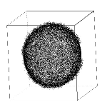
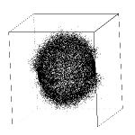
By introducing the term $dR$ the temperature anisotropies are transformed to variations in the radial direction around the sphere. The normalisation ensures that $dR$ has zero mean and a standard deviation of $a$. The parameters $R$ and $a$ are free (scale) parameters, which control the size of the temperature-induced radial jitter relative to its spatial extent. These two parameters $R$ and $a$, together with the scaling range parameter $r$ for the calculation of the scaling indices have to be properly set so that the scaling indices are sensitive to the temperature fluctuations in the chosen (spatial) scaling range (see Figure 5).

Figure 5: Left: WMAP-data represented as a three-dimensional point distribution. Right: $x,z$-projection of all points with $|y|<0.05$. Above: $a=0.075$, below: $a=0.225$. The black circles indicate the scaling ranges $r=0.075$ and $r=0.225$ respectively. A good sensitivity to the temperature fluctuations at a given scale $r$ is obtained for $r=a$.

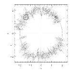
To achieve this, we coupled the parameter $a$, which controls the width of the radial jitter with the scaling range $r$ and set for each scaling range $a=r$. The size of the the sphere $R$ has to be chosen large enough with respect to the radial jitter $dR$, so that the scaling indices remain a local measure and their calculation are not affected by pixels on the opposite side of the sphere with a large $dR$. Hence, we deliberately set $R=2$ for all calculations presented below. We performed some tests for the WMAP data and a subset of simulations using different values of $R$, e.g. $R=1.5$, and found only marginal differences in the results.
Figure 5 shows the representation of the WMAP data as a point set $P=\{\vec{p_{i}}=(x_{i},y_{i},z_{i})\},i=1,\ldots,N_{pixel}$ and two-dimensional projections of all data with $|y|<0.05$. For each point $p_{i}$ a set of weighted scaling indices $\alpha$ for ten different values of $r$, $r=0.025,0.05,0.75,\ldots,0.25$ is calculated, which (roughly) corresponds an angular resolution $\psi$ of $\psi=1.4^{\circ},2.8^{\circ},\ldots,14.3^{\circ}$.
Thus, the weighted scaling indices can also be interpreted as a filter response of a local nonlinear filter acting on the spherical CMB data. Global quantities of the $\alpha$-distribution as well as the probability density $P(\alpha)$ are used to derive statistics quantifying the structures in the WMAP-data and respective simulations.

4 Results

Figure 6: From top to bottom: Co-added WMAP-map with Kp0-mask, color-coded $\alpha$-response for $r=0.175$ and $r=0.225$ and Kp0- and extended mask.

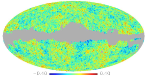
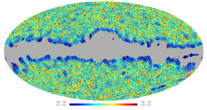
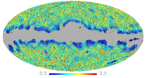
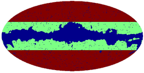
In Figure 6 the preprocessed foreground-cleaned coadded map of the WMAP data and the $\alpha$- response for two different radii $r$ is shown. It is obvious that for these larger scales the pixels in the vicinity of the Kp0-mask are affected by boundaries effects, which lead to systematically lower values for $\alpha$. This effect, which is only due to the lack of data points within the Kp0 mask, is the same for both the WMAP-data and the simulations, so that global measures based on the scaling indices, e.g. the moments of the probability distribution, are systematically affected in the same way. However, some smaller local effects may be diluted by the boundary effects. In order to have a cleaner map we also considered only scaling indices in a more conservative mask, where only pixels with $\left|b\right|>30$ ($b$: Galactic latitude) were selected (Figure 6). Note that for the calculation of the scaling indices all pixels outside the Kp0-mask were taken into account. In the following we always explicitly specify to which chosen mask the presented results refer.

Figure 7: Probability density $P(\alpha)$ for the co-added WMAP data and $20$ simulations for $r=0.175$ and the Kp0-mask.

Figure 8: Same as Figure 7 but for the extended mask.

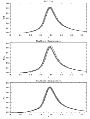
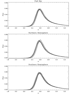
The probability densities $P(\alpha)$ of the scaling indices for one selected scale ($r=0.175$) and both masks are displayed in the Figures 7 and 8 for the WMAP-data and a subset of 20 simulations. One immediately realizes that for both masks the probability density for the WMAP data is shifted towards higher values, which indicates that the underlying temperature fluctuations for the observed data resemble more ’unstructured’, i.e. purely random and uniform fluctuations than the simulations. This effect is more pronounced in the northern hemisphere than in the southern. Furthermore, the distributions are broader for the simulations than for the WMAP-data, indicating that the simulations exhibit a larger structural variability than the observed data.

Figure 9: Scaling index mean statistics as a function of the scaling range $r$ for the full sky (above), northern (middle) and southern hemisphere (below) using the Kp0-mask. $+$ denote the values for WMAP, the dark gray and light gray areas indicate the $1\sigma$ and $3\sigma$ regions around the mean value (black line) as derived from the simulations.

Figure 10: Same as fig. 9 but for the standard deviation $\sigma_{\alpha}$.

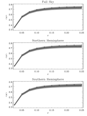
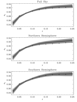
These effects can more rigorously be quantified by calculating the mean and standard deviation for the distribution of scaling indices as calculated for different scaling ranges. Figures 9 and 10 show these results. For scales larger than $r=0.1$ the mean of the scaling indices is always systematically higher for the WMAP than for the simulations. The effect is much more pronounced in the northern hemisphere. For the standard deviation we observe for the same scales significantly lower values for WMAP in the northern hemisphere and slightly higher ones for the southern sky. For the full sky these two effects cancel each other so that the observed deviations to lower values are no longer so significant.
Beside the mean and standard deviation we additionally considered a combination of these two test statistics, namely a diagonal $\chi^{2}$-statistic

$$\chi^{2}=\sum_{i=1}^{2}\left[\frac{M_{i}-<M_{i}>}{\sigma_{M_{i}}}\right]^{2}\;,$$ (19)

where $M_{1}=<\alpha>$ and $M_{2}=\sigma_{\alpha}$. This statistic is computed for both the simulations and the observed moments. Note that we follow the reasoning of Eriksen et al. (2004a) and choose a diagonal $\chi^{2}$-statistics, because also in our case the moments are highly correlated leading to high values in the off-diagonal elements of the cross-correlation matrix. But if the chosen model is a proper description of the data, any combination of measures should yield statistically the same values for the observations and the simulations. The significances of the deviations of the WMAP-data from the simulations

$$S=\left|\frac{M-<M>}{\sigma_{M}}\right|$$ (20)

($M=<\alpha>,\sigma_{\alpha}$ and $\chi^{2}$) are shown in Figures 11 and 12 for the Kp0-mask and the extended mask.

Figure 11: Significances of the (combined) moments of the $\alpha$-distribution of the WMAP-data with the Kp0-mask as a function of the scaling range $r$. $+$ denotes the mean, $\star$ the standard deviation and the boxes $\chi^{2}$-combination of the mean and standard deviation.

Figure 12: Same as Fig. 11 but for the extended mask.

The mean $<M>$ and standard deviation $\sigma_{M}$ of the three measures $M$ were derived from the set of simulations.
As a pure frequentist approach, we also considered the confidence or significance level of the null hypothesis that the observation belongs to the Gaussian Monte Carlo ensemble and consider the fraction of simulations $p$, which have higher (lower) values of $M$ than the moments for the observation. In the Tables 1, 2 and 3 the significances $S$ as well as the probabilities $p$ are listed.

Table 1: $<\alpha>$ with Kp0 mask

Scaling Range	Full Sky	Northern Sky	Southern Sky
($r$)	($S$/%)	($S$/%)	($S$/%)
0.025	2.2/99.5	2.1/99.4	2.3/99.8
0.050	2.1/99.8	2.0/99.3	2.2/99.7
0.075	2.0/99.5	1.9/99.3	2.0/99.4
0.100	2.0/99.4	2.0/99.7	1.9/98.8
0.125	2.0/99.5	2.1/99.8	1.9/98.6
0.150	2.1/99.6	2.4/99.9	1.8/98.4
0.175	2.2/99.7	2.5/$>$99.9	1.7/97.4
0.200	2.2/99.7	2.7/$>$99.9	1.6/96.0
0.225	2.2/99.7	2.7/$>$99.9	1.5/94.0
0.250	2.1/99.4	2.8/$>$99.9	1.3/91.6

Table 2: $\sigma_{\alpha}$ with Kp0 mask

Scaling Range	Full Sky	Northern Sky	Southern Sky
($r$)	($S$/%)	($S$/%)	($S$/%)
0.025	2.0/98.9	1.9/98.7	1.9/98.9
0.050	2.2/99.7	2.0/98.9	2.1/99.1
0.075	0.4/64.8	0.2/60.3	0.4/63.8
0.100	1.6/94.9	1.5/94.2	0.9/81.6
0.125	2.2/99.0	2.6/99.8	1.0/84.6
0.150	2.3/99.0	2.9/99.9	0.8/79.5
0.175	2.1/98.4	2.9/99.9	0.6/71.6
0.200	1.9/97.5	2.8/99.9	0.5/66.8
0.225	1.7/95.8	2.6/99.7	0.4/64.3
0.250	1.5/93.1	2.4/99.7	0.2/58.3

Table 3: $\chi^{2}$ with Kp0 mask

Scaling Range	Full Sky	Northern Sky	Southern Sky
($r$)	($S$/%)	($S$/%)	($S$/%)
0.025	2.0/96.7	1.8/95.9	2.1/96.9
0.050	2.3/97.5	2.0/96.1	2.4/97.7
0.075	0.9/88.4	0.7/85.9	1.0/88.4
0.100	1.8/95.4	1.7/94.9	1.1/89.3
0.125	2.7/97.8	3.6/98.9	1.0/89.2
0.150	2.9/98.2	4.8/99.3	0.8/85.7
0.175	2.7/97.9	5.2/99.4	0.5/80.3
0.200	2.5/97.1	5.1/99.3	0.3/76.4
0.225	2.1/96.6	4.8/99.3	0.1/70.1
0.250	1.8/94.7	4.5/99.0	0.1/63.0

Analysing the significances and the confidence levels of the (combined) moments of the distribution of scaling indices as a function of the scaling range the results read as follows: For the full sky we obtain for the mean value $<\alpha>$ significances ranging from $2.0$ to $2.2$ for the different scales. The confidence levels for the detection of non-Gaussianties are, however, very high and do not fall below $99\%$ for any scale. A closer look at the distribution of $<\alpha>$ for the simulations reveals that this distribution is not Gaussian but we find a number of outliers with very high values for $<\alpha>$, which leads to high $\sigma_{<\alpha>}$ thus to low significances. So although the significances for detecting non-Gaussianities are not very high, the confidence levels, for which no implicit assumptions about the distribution function of the test statistics is made, strongly indicate the presence of non-Gaussian features in the observed WMAP-data. Even higher values for both the significances and the confidence levels are found, if one only considers the northern hemisphere. In this case the sigificances range from $1.9$ for smaller scales to $2.8$ for the largest scale. For scales larger than $r=0.15$ none of the simulations was found to have a higher values for $<\alpha>$ than the observation, which represents a quite unambigous detection of non-Gaussianties in the northern hemisphere. For the southern hemisphere, however, both the significances and the confidence levels for the smaller radii are slighly higher than for the northern sky but continously decrease for higher radii $r$. For the standard deviation we find slighly different results. For the smallest scales ($r=0.025$) $\sigma_{\alpha}$ is significantly larger for WMAP than for the simulations. In a transition regime $r\approx 0.075$ the standard deviation is practically the same for the observation and the Monte Carlo sample. For larger scales we observe higher standard deviations for the simulations. This effect is much more pronounced in the northern hemisphere giving rise to significances up to $2.9$ and very high confidence levels for intermediate scales. For the largest scales the differences for $\sigma$ between simulations and oberservation diminishes. For the southern hemisphere the width of the distributions become more and more similar so that no signatures for deviations from Gaussianity are identified using $\sigma_{\alpha}$. The behaviour of the $\chi^{2}$- statistics as a function of the scale parameters $r$ can – as expected – be regarded as a superposition of the two underlying statistics $<\alpha>$ and $\sigma_{\alpha}$. Only the significances are highly increased leading to a $5\sigma$ detection of non-Gaussianity at scales of $r=0.175$ in the northern sky. Performing the same analyses for the extended mask (Figure 12) yields essentially the same results. Only marginal variations for the significances and confidence levels (which are not explicitly shown in this paper) are found in this case. Thus, these results are quite stable with respect to differences for the chosen mask.
Some readers might argue that the selection of the moments and especially of the scales, where the significances are largest, represents an a posteriori choice taken after looking at the data. However, the choice of the moments was motivated by the results obtained with simulations (see Section 3) and the investigation of the data on different length scales can be regarded as a fairly conventional and unbiased approach. If a random field is Gaussian, it must be Gaussian on all scales. If deviations are detected at some scales, one can already infer non-Gaussianity. Nevertheless, we also calculated diagonal $\chi^{2}$-statistics, where we considered only one (mean or standard deviation) or both measures, and summed over all length scales ,

$$\chi^{2}_{<\alpha>}=\sum_{i=1}^{N_{r}}\left[\frac{M_{1}(r_{i})-<M_{1}(r_{i})>}{\sigma_{M_{1}(r_{i})}}\right]^{2}$$ (21)

$$\chi^{2}_{\sigma_{\alpha}}=\sum_{i=1}^{N_{r}}\left[\frac{M_{2}(r_{i})-<M_{2}(r_{i})>}{\sigma_{M_{1}(r_{i})}}\right]^{2}$$ (22)

$$\chi^{2}_{<\alpha>,\sigma_{\alpha}}=\sum_{i=1}^{N_{r}}\sum_{j=1}^{2}\left[\frac{M_{j}(r_{i})-<M_{j}(r_{i})>}{\sigma_{M_{j}(r_{i})}}\right]^{2}$$ (23)

with $M_{1}(r_{i})=<\alpha(r_{i})>$, $M_{2}(r_{i})=\sigma_{\alpha}(r_{i})$ and $N_{r}$ being the number of considered length scales (here: $N_{r}=10$). The results are summarised in Table 4.

Table 4: $\chi^{2}$, all scales

$\chi^{2}$	Full Sky	Northern Sky	Southern Sky
	($S$/%)	($S$/%)	($S$/%)
$\chi^{2}_{<\alpha>}$	2.1/96.9	2.7/97.7	1.5/94.2
$\chi^{2}_{\sigma_{\alpha}}$	2.4/96.5	4.4/99.5	0.2/70.0
$\chi^{2}_{<\alpha>,\sigma_{\alpha}}$	2.4/97.3	3.7/98.9	1.1/91.6

Also for this obviously a priori test statistics, where some unimportant scales contribute to the final value of $\chi^{2}$ and may dilute the result, we find significant signatures for non-Gaussianities in the northern sky.
Beside the previous analyses based on global measures derived from the $P(\alpha)$- distribution, we also investigate the spectrum of scaling indices on a differential level. Therefore we consider the bin-wise significances $S(\alpha_{i})$,

$$S(\alpha_{i})=\ \frac{P(\alpha_{i})-<P(\alpha_{i})>}{\sigma_{P(\alpha_{i})}}$$ (24)

for the probability densities $P(\alpha)$ of selected scales (see Figures 13 and 14).

Figure 13: Bin-wise significances (with sign) as derived from the pribability distribution $P(\alpha)$ for the WMAP data and Kp0-mask for $r=0.175$ (above) and $r=0.225$ (below).

Figure 14: Same as fig. 13 but for the extended mask.

Note that we omitted in this case the absolute value in the definition of the significance in order to show in which direction with respect to the simulations the $P(\alpha)$ of the WMAP data deviates. Although the spectra for the Kp0-mask (Figure 13) are diluted by edge effects for smaller $\alpha$, one can clearly detect the sharp transition from systematically small to high values in the significances, which is due to the shift of the whole spectrum towards higher $\alpha$-values for the WMAP-data. This shift is so pronounced that for some bins of the spectrum even the $3\sigma$- level for the deviation is nearly reached. If we consider the same spectra for the extended mask, where almost all disturbing edge effects are removed, we see (Figure 14) - beside the transition from negative to positive values due to the global shift - a new, highly significant feature at $\alpha\approx 2.1$ in the southern sky emerging, when the scaling range is increased. There is an excess of pixels with these low $\alpha-$values in the WMAP-data as compared to the simulated maps. To elucidate the origin of these pixels we color-coded the pixels according their value of scaling indices (Figure 15).

Figure 15: Marked pixels with $\alpha\in[2.0,2.3]$ (yellow), $\alpha\in[2.425,2.475]$ (blue) and $\alpha\in[2.60,2.65]$ (red) for $r=0.175$ (above) and $r=0.225$ (below).

Figure 16: Significanes of the (rotated) upper hemisphere for the SIM based statistics for $r=0.175$. From top to bottom: mean $<\alpha>$, standard deviation $\sigma_{\alpha}$ and $\chi^{2}$-combination of mean and standard deviation. The highest significances were obtained for $(\theta,\phi)=(27^{\circ},35^{\circ})$ for $<\alpha>$, $(\theta,\phi)=(39^{\circ},45^{\circ})$ for $\sigma_{\alpha}$ and $(\theta,\phi)=(30^{\circ},41^{\circ})$ for $\chi^{2}$. The maximal asymmetry between the rotated northern and southern hemisphere were found for the rotation angles $(\theta,\phi)=(27^{\circ},35^{\circ})$ for $<\alpha>$, $(\theta,\phi)=(30^{\circ},41^{\circ})$ for $\sigma_{\alpha}$ and $(\theta,\phi)=(30^{\circ},41^{\circ})$ for $\chi^{2}$.

Figure 17: Same as Fig. 16 but for $r=0.225$. For this scaling range, the highest significances were obtained for $(\theta,\phi)=(21^{\circ},148^{\circ})$ for $<\alpha>$), $(\theta,\phi)=(27^{\circ},65^{\circ})$ for $\sigma_{\alpha}$ and $(\theta,\phi)=(30^{\circ},41^{\circ})$ for $\chi^{2}$. The maximal asymmetries between the rotated northern and southern hemisphere were found for the rotation angles $(\theta,\phi)=(21^{\circ},148^{\circ})$ for $<\alpha>$, $(\theta,\phi)=(27^{\circ},55^{\circ})$ for $\sigma_{\alpha}$ and $(\theta,\phi)=(30^{\circ},41^{\circ})$ for $\chi^{2}$.

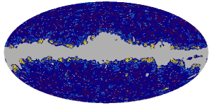
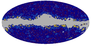
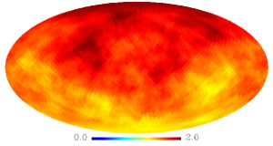
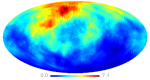
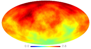
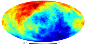
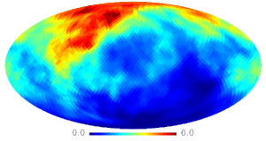
It becomes immediately obvious that the pixels with the small $\alpha$-values identified in the southern sky form two to three clusters (depending on the scale $r$), where the largest one corresponds to the cold spot – the well-known anomaly first detected by Vielva et al. (2004) by means of a wavelets analysis. The pixels belonging to the other two $\alpha$-intervals, for which the largest deviations in the bulge of the distribution are found, cannot be associated with special localised features. These pixels are rather distributed all over the sky, which indicates that the shift of the spectrum of scaling indices represents a global intrinsic effect.
The distinction between northern and southern hemisphere, which we made during the previous analysis, is natural being triggered by excluding the foreground-contamined area of the galactic plane. On the other hand, this choice is arbitrary, because no symmetry axis is preferable for a presumably isotropic CMB. To test for asymmetries in WMAP-data we consider rotated hemispheres, calculate the global measures $<\alpha>,\sigma_{\alpha}$ and $\chi^{2}$ for $3072$ rotation angles and compare the results for the (rotated) northern and southern hemispheres. In Figures 16 and 17 we show the significances $S(<\alpha>)$, $S(\sigma_{\alpha})$ and $S(\chi^{2})$ of the northern hemisphere as determined in a reference frame where the north pole pierces the center of the color-coded pixel. All three measures yield systematically higher significances for rotations pointing to northern directions relative to the galactic coordinate system. The rotation angles, for which the highest significances of the northern hemisphere are obtained, are listed in the captions of the respective figures. They are very similar but do not always coincide with the rotations, for which the maximal asymmetries, as measured by the difference of the significances of the rotated northern and southern hemisphere are found. It is worth noticing that the direction of the most pronounced non-Gaussianities and asymmetries differs from the dipole direction $(\theta,\phi)=(42^{\circ},264^{\circ})$ and the so-called axis of evil $(\theta,\phi)=(30^{\circ},260^{\circ})$, which is very close to the dipole direction.

5 Summary

We performed a scaling index analysis of the WMAP three-year data. Specifically, we analysed the foreground-cleaned co-added maps of the V-and W-band. We found highly significant signatures of both non-Gaussianities and asymmetries in the WMAP three-year data. Our main findings can be summarized and interpreted as follows:
In the northern hemisphere the spectrum of scaling indices is systematically broader and shifted towards higher values yielding highly significant deviations of the mean and standard deviation of the distribution. This effect can naturally be interpreted as too few structure and structural variations in the CMB-fluctuations as measured by WMAP compared to the predicted ones within the concordance model. The highest global signatures for non-Gaussianities and asymmetries between the northern and southern hemisphere were found for rotated coordinate systems, where the significances for the detection of signatures for non-Gaussianities range from $2.6\sigma$ up to $7.4\sigma$. These findings are quite consistent with previous results for the first year data (Eriksen et al., 2004a, b; Park, 2004), where very similar features were identified – even though with a smaller significance level – using the Minkowski functionals, the power spectrum and $N$-point correlation functions.
In the southern hemisphere the global properties of the $P(\alpha)$ distribution for the WMAP-data are more consistent with the simulations than in the northern sky. We find, however, highly significant localisable features of non-Gaussianity, for which the largest one can be associated with a cold spot. An anomalous area detected by Vielva et al. (2004) in the WMAP first year data and confirmed in the WMAP three year data (Cruz et al., 2006).

6 Conclusions

In conclusion, we demonstrated for the first time the feasibility to adapt and apply the scaling index method as an estimator of local scaling properties of a point set to spherical symmetric data.
The results obtained with the scaling indices give further strong evidence that also the coadded WMAP three year data do indeed contain unusual features, which are not in agreement with the hypotheses of Gaussianity and isotropy predicted in the standard inflationary scenario.
A quite remarkable result of our study is the fact that two previously known anomalies, namely the lack of structure in the northern sky and the cold spot in the southern hemisphere could be reidentified using a completely different test statistic. This increases the evidence that these anomalies are of true physical origin and not related to one single test statistic.
It is also worth noticing that the scaling indices could detect both of these anomalies simultaneously, whereas the wavelets were only sensitive to localised spot-like structures and the $N$-point correlation functions and Minkowski-functionals only detected the non-Gaussianities and asymmetries on large scales.
The main task for future studies is to elucidate the possible sources of these anomalies, whether they are due to systematics or foreground effects or truely represent intrinsic CMB-fluctuations due to some exotic physics. Future more detailed studies will investigate the possible origins of the non-Gaussian signatures by separately analysing the V and W bands and by comparing the three year WMAP-data with the first, second and third year data. All these tests may help to find hints about the origin of the non-Gaussian signatures.
In either case we could demonstrate that the scaling index method provides very flexible and highly sensitive statistics for e.g. the identification of asymmetries and non-Gaussian signatures in the WMAP-data thus representing an important novel statistical tool for CMB analyses.

References

- Acquaviva et al. (2003) Acquaviva V., Bartolo N., Matarresse S., Riotto A., 2003, Nucl. Phys. B, 667, 119
- Albrecht & Steinhard (1982) Albrecht A., Steinhard P.J., 1982, Phys. Rev. Lett., 48, 1220
- Bennett et al. (2003) Bennett C. L., et al., 2003, ApJS, 148, 1
- Bernardeau & Uzan (2002) Bernardeau F., Uzan J.-P., 2002, Phys. Rev. D, 66, 103506
- Bouchet, Bennett, & Stebbins (1988) Bouchet F. R., Bennett D. P., Stebbins, A., 1988, Nature, 335, 410
- Bridges et al. (2006) Bridges M., McEwen, J.D., Lasenby A. N., Hobson, M.P., 2006, astro-ph/0605325
- Chiang et al. (2003) Chiang L.-Y., Naselsky P. D., Verkhodanov O. V., Way, M. J., 2003, ApJ, 590, L65
- Coles et al. (2004) Coles P., Dineen P., Earl J., Wright D., 2004, MNRAS, 350, 989
- Copi et al. (2004) Copi C. J., Huterer D., & Starkman G. D., 2004, Phys. Rev. D, 70, 043515
- Copi et al. (2006) Copi C. J., Huterer D., Schwarz D. J., Starkman G. D., 2006, astro-ph/0605135
- Cruz et al. (2006) Cruz M., Cayón L., Martínes-Gonzaléz E., Vielva P., Jin, J., 2006, astro-ph/0603859
- Cruz et al. (2005) Cruz M., Martínes-Gonzaléz E., Vielva P., Cayón, L., 2005, MNRAS, 356, 29
- de Oliveira-Costa et al. (2004) de Oliveira-Costa A., Tegmark M., Zaldarriaga M., Hamilton A., 2004, Phys. Rev. D, 69, 063516
- Eriksen et al. (2004a) Eriksen H. K., Novikov D. I., Lilje P. B., Banday A. J., Górski K. M., 2004, ApJ, 612, 64
- Eriksen et al. (2004b) Eriksen H. K., Hansen F. K., Banday A. J., Górski K. M., Lilje, P. B., 2004, ApJ, 605, 14
- Eriksen et al. (2005a) Eriksen H. K., Banday A. J., Górski K. M., Lilje P. B., 2005, ApJ, 622, 58
- Gliozzi, Papadakis, & Räth (2006) Gliozzi M., Papadakis I. E., & Räth C. 2006 A & A, 449, 969
- Gliozzi, et al. (2002) Gliozzi, M. et al. 2002 A & A, 391, 875
- Górski et al. (2005) Górski K. M, Hivon E., Banday A. J., Wandelt B. D., Hansen F. K., Reinecke M., Bartelmann M., 2005, ApJ, 622, 759
- Guth (1981) Guth A. H., Phys. Rev. D, 23, 347
- Hansen, Banday, & Górski (2004) Hansen F. K., Banday A. J., Górski, K. M., 2004, MNRAS, 354, 641
- Hinshaw et al. (2006) Hinshaw G. et al., 2006, astro-ph/0603451
- Jaffe et al. (2006) Jaffe T. R., Banday A. J., Eriksen H. K., Górski K. M., Hansen F. K. 2006, A & A, 460, 393
- Jamitzky et al. (2001) Jamitzky F. et al. 2001, Ultramicroscopy, 86, 241
- Komatsu et al. (2003) Komatsu E. et al., 2003, ApJS, 148, 119
- Land (2005) Land K., Magueijo J., 2005, Phys. Rev. Lett., 95, 071301
- Land (2006) Land K., Magueijo J., 2006, astro-ph/0611518
- Linde (1982) Linde A. H., 1982 Phys. Lett. B, 108, 389
- Linde & Mukhanov (1997) Linde A. H., Mukhanov V., 1997, Phys. Rev. D, 56, R535
- Martínez-González et al. (2002) Martínez-González E., Gallegos J. E., Argüeso F., Cayón L., Sanz J. L., 2002, MNRAS, 336, 22
- Martínez-González et al. (2006) Martínez-González E., Cruz M., Cayón L., Vielva P., 2006, New Astron. Review, 50, 875
- McEwen et al. (2005) McEwen J. D., Hobson M. P., Lasenby A. N., Mortlock D. J., 2005, MNRAS, 359, 1583
- Monetti et al. (2003) Monetti R., et al., 2003, Proc. of the SPIE, 5032, 1777
- Mueller et al. (2004) Mueller D., et al., 2004, Proc. of the SPIE, 5370, 225
- Naselsky et al. (2005) Naselsky P. D., Chiang L.-Y., Olesen P., Novikov I., 2005, Phys. Rev. D, 72, 063512
- Park (2004) Park C.-G., 2004, MNRAS, 349, 313
- Peebles (1997) Peebles P.J.E., 1997, ApJ, 483, L1
- Räth & Schuecker (2003) Räth C., Schuecker P., 2003, MNRAS, 344, 115
- Räth et al. (2002) Räth C., Bunk W., Huber M. B., Morfill G. E., Retzlaff J., Schuecker, P. 2002, MNRAS, 337, 413
- Spergel et al. (2003) Spergel D. N., et al. 2003, ApJS, 148, 175
- Spergel et al. (2006) Spergel D. N., et al., 2006, astro-ph/0603449
- Turok (1996) Turok N., 1996, ApJ, 473, L5
- Turok, & Spergel (1990) Turok, N., Spergel D., 1990, Phys. Rev. Lett., 64, 2736
- Vielva et al. (2004) Vielva P., Martínes-Gonzaléz E., Barreiro R. B., Sanz J. L., Cayón L., 2004, ApJ, 609, 22