The Bullet Cluster 1E0657-558 evidence shows Modified Gravity
in the absence of Dark Matter

Abstract

A detailed analysis of the November 15, 2006 data release (Clowe et al., 2006a; Bradač et al., 2006; Clowe et al., 2006c, b) X-ray surface density $\Sigma$-map and the strong and weak gravitational lensing convergence $\kappa$-map for the Bullet Cluster 1E0657-558 is performed and the results are compared with the predictions of a modified gravity (MOG) and dark matter. Our surface density $\Sigma$-model is computed using a King $\beta$-model density, and a mass profile of the main cluster and an isothermal temperature profile are determined by the MOG. We find that the main cluster thermal profile is nearly isothermal. The MOG prediction of the isothermal temperature of the main cluster is $T=15.5\pm 3.9\ \mbox{keV}$, in good agreement with the experimental value $T=14.8^{+2.0}_{-1.7}\ \mbox{keV}$. Excellent fits to the two-dimensional convergence $\kappa$-map data are obtained without non-baryonic dark matter, accounting for the $8\sigma$ spatial offset between the $\Sigma$-map and the $\kappa$-map reported in Clowe et al. (2006a). The MOG prediction for the $\kappa$-map results in two baryonic components distributed across the Bullet Cluster 1E0657-558 with averaged mass-fraction of 83% intracluster medium (ICM) gas and 17% galaxies. Conversely, the Newtonian dark matter $\kappa$-model has on average 76% dark matter (neglecting the indeterminant contribution due to the galaxies) and 24% ICM gas for a baryon to dark matter mass-fraction of $0.32$, a statistically significant result when compared to the predicted $\Lambda$-CDM cosmological baryon mass-fraction of $0.176^{+0.019}_{-0.012}$ (Spergel et al., 2007).

I Introduction

I.1 The Question of Missing Mass

Galaxy cluster masses have been known to require some form of energy density that makes its presence felt only by its gravitational effects since Zwicky (1933) analysed the velocity dispersion for the Coma cluster. Application of the Newtonian $1/r^{2}$ gravitational force law inevitably points to the question of missing mass, and may be explained by dark matter (Oort, 1932). The amount of non-baryonic dark matter required to maintain consistency with Newtonian physics increases as the mass scale increases so that the mass to light ratio of clusters of galaxies exceeds the mass to light ratio for individual galaxies by as much as a factor of $\sim 6$, which exceeds the mass to light ratio for the luminous inner core of galaxies by as much as a factor of $\sim 10$. In clusters of galaxies, the dark matter paradigm leads to a mass to light ratio as much as $300\ M_{\odot}/L_{\odot}$. In this scenario, non-baryonic dark matter dominates over baryons outside the cores of galaxies (by $\approx 80-90\%$).

Dark matter has dominated cosmology for the last five decades, although the search for dark matter has to this point come up empty. Regardless, one of the triumphs of cosmology has been the precise determination of the standard (power-law flat, $\Lambda$-CDM) cosmological model parameters. The highly anticipated third year results from the WMAP team have determined the cosmological baryon mass-fraction (to non-baryonic dark matter) to be $0.176^{+0.019}_{-0.012}$ (Spergel et al., 2007). This ratio may be inverted, so that for every gram of baryonic matter, there are 5.68 grams of non-baryonic dark matter – at least on cosmological scales. There seems to be no evidence of dark matter on the scale of the solar system, and the cores of galaxies also seem to be devoid of dark matter.

Galaxy clusters and superclusters are the largest virialized (gravitationally bound) objects in the Universe and make ideal laboratories for gravitational physicists. The data come from three sources:

1. X-ray imaging of the hot intracluster medium (ICM),

2. Hubble, Spitzer and Magellan telescope images of the galaxies comprising the clusters,

3. strong and weak gravitational lensing surveys which may be used to calculate the mass distribution projected onto the sky (within a particular theory of gravity).

The alternative to the dark matter paradigm is to modify the Newtonian $1/r^{2}$ gravitational force law so that the ordinary (visible) baryonic matter accounts for the observed gravitational effect. An analysis of the Bullet Cluster 1E0657-558 surface density $\Sigma$-map and convergence $\kappa$-map data by Angus et al. (2006, 2007) based on Milgrom s Modified Newtonian Dynamics (MOND) model (Milgrom, 1983; Sanders and McGaugh, 2002) and Bekenstein’s relativistic version of MOND (Bekenstein, 2004) failed to fit the data without dark matter. More recently, further evidence that MOND needs dark matter in weak lensing of clusters has been obtained by Takahashi and Chiba (2007). Problems with fitting X-ray temperature profiles with Milgrom s MOND model without dark matter were shown in  Aguirre et al. (2001); Sanders (2006); Pointecouteau and Silk (2005); Brownstein and Moffat (2006a). Neutrino matter with an electron neutrino mass $m_{\nu}\sim 2\ \mbox{eV}$ can fit the bullet cluster data (Angus et al., 2006, 2007; Sanders, 2006). This mass is at the upper bound obtained from observations. The Karlsruhe Tritium Neutrino (KATRIN) experiment will be able to falsify 2 eV electron neutrinos at 95% confidence level within months of taking data in 2009.

The theory of modified gravity – or MOG model – based upon a covariant generalization of Einstein’s theory with auxiliary (gravitational) fields in addition to the metric was proposed in Moffat (2005, 2006b) including metric skew-tensor gravity (MSTG) theory and scalar-tensor-vector gravity (STVG) theory. Both versions of MOG, MSTG and STVG, modify the Newtonian $1/r^{2}$ gravitational force law in the same way so that it is valid at small distances, say at terrestrial scales.

Brownstein and Moffat (2006b) applied MOG to the question of galaxy rotation curves, and presented the fits to a large sample of over 100 low surface brightness (LSB), high surface brightness (HSB) and dwarf galaxies. Each galaxy rotation curve was fit without dark matter using only the available photometric data (stellar matter and visible gas) and alternatively a two-parameter mass distribution model which made no assumption regarding the mass to light ratio. The results were compared to MOND and were nearly indistinguishably right out to the edge of the rotation curve data, where MOND predicts a forever flat rotation curve, but MOG predicts an eventual return to the familiar $1/r^{2}$ gravitational force law. The mass to light ratio varied between $2-5\ M_{\odot}/L_{\odot}$ across the sample of 101 galaxies in contradiction to the dark matter paradigm which predicts a mass to light ratio typically as high as $50\ M_{\odot}/L_{\odot}$.

In a sequel, Brownstein and Moffat (2006a) applied MOG to the question of galaxy cluster masses, and presented the fits to a large sample of over 100 X-ray galaxy clusters of temperatures ranging from 0.52 keV (6 million kelvin) to 13.29 keV (150 million kelvin). For each of the 106 galaxy clusters, the MOG provided a parameter-free prediction for the ICM gas mass profile, which reasonably matched the X-ray observations (King $\beta$-model) for the same sample compiled by Reiprich (2001) and Reiprich and Böhringer (2002). The MOND predictions were presented for each galaxy cluster, but failed to fit the data. The Newtonian dark matter result outweighed the visible ICM gas mass profiles by an order of magnitude.

In the solar system, the Doppler data from the Pioneer 10 and 11 spacecraft suggest a deviation from the Newtonian $1/r^{2}$ gravitational force law beyond Saturn’s orbit. Brownstein and Moffat (2006c) applied MOG to fit the available anomalous acceleration data (Nieto and Anderson, 2005) for the Pioneer 10/11 spacecraft. The solution showed a remarkably low variance of residuals corresponding to a reduced $\chi^{2}$ per degree of freedom of 0.42 signalling a good fit. The magnitude of the satellite acceleration exceeds the MOND critical acceleration, negating the MOND solution (Sanders, 2006). The dark matter paradigm is severely limited within the solar system by stability issues of the sun, and precision gravitational experiments including satellite, lunar laser ranging, and measurements of the Gaussian gravitational constant and Kepler’s law of planetary motion. Without an actual theory of dark matter, no attempt to fit the Pioneer anomaly with dark matter has been suggested. Remarkably, MOG provides a closely fit solution to the Pioneer 10/11 anomaly and is consistent with the accurate equivalence principle, all current satellite, laser ranging observations for the inner planets, and the precession of perihelion for all of the planets.

A fit to the acoustical wave peaks observed in the cosmic microwave background (CMB) data using MOG has been achieved without dark matter. Moreover, a possible explanation for the accelerated expansion of the Universe has been obtained in MOG (Moffat, 2007).

Presently, on both an empirical and theoretical level, MOG is the most successful alternative to dark matter. The successful application of MOG across scales ranging from clusters of galaxies (Megaparsecs) to HSB, LSB and dwarf galaxies (kiloparsecs), to the solar system (AU’s) provides a clue to the question of missing mass. The apparent necessity of the dark matter paradigm may be an artifact of applying the Newtonian $1/r^{2}$ gravitational force law to scales where it is not valid, where a theory such as MOG takes over. The “excess gravity” that MOG accounts for may have nothing to do with the hypothesized missing mass of dark matter. But how can we distinguish the two? In most observable systems, gravity creates a central potential, where the baryon density is naturally the highest. So in most situations, the matter which is creating the gravity potential occupies the same volume as the visible matter. Clowe et al. (2006c) describes this as a degeneracy between whether gravity comes from dark matter, or from the observed baryonic mass of the hot ICM and visible galaxies where the excess gravity is due to MOG. This degeneracy may be split by examining a system that is out of steady state, where there is spatial separation between the hot ICM and visible galaxies. This is precisely the case in galaxy cluster mergers: the galaxies will experience a different gravitational potential created by the hot ICM than if they were concentrated at the center of the ICM. Moffat (2006a) considered the possibility that MOG may provide the explanation of the recently reported “extra gravity” without non-baryonic dark matter which has so far been interpreted as direct evidence of dark matter. The research presented here addresses the full-sky data product for the Bullet Cluster 1E0657-558, recently released to the public (Clowe et al., 2006b).

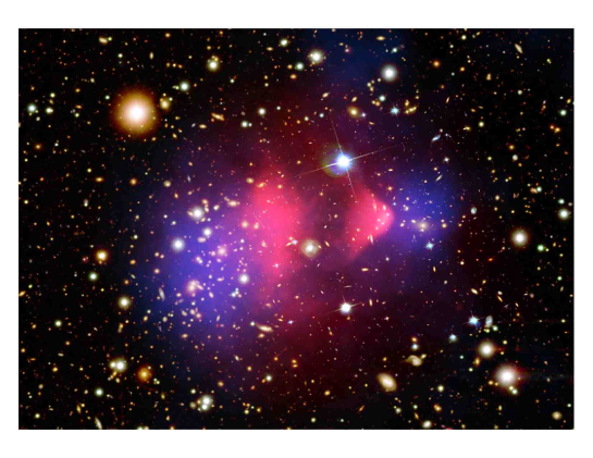
Figure 1: False colour image of Bullet Cluster 1E0657-558.The surface density $\Sigma$-map reconstructed from X-ray imaging observations is shown in red and the convergence $\kappa$-map as reconstructed from strong and weak gravitational lensing observations is shown in blue. Image provided courtesy of Chandra X-ray Observatory.

I.2 The Latest Results from the Bullet Cluster 1E0657-558

• The Chandra Peer Review has declared the Bullet Cluster 1E0657-558 to be the most interesting cluster in the sky. This system, located at a redshift $z=0.296$ has the highest X-ray luminosity and temperature ($T=14.1\pm 0.2\ \mbox{keV}\sim 1.65\times 10^{8}\ \mbox{K}$), and demonstrates a spectacular merger in the plane of the sky exhibiting a supersonic shock front, with Mach number as high as $3.0\pm 0.4$ (Markevitch, 2006). The Bullet Cluster 1E0657-558 has provided a rich dataset in the X-ray spectrum which has been modeled to high precision. From the extra-long $5.2\times 10^{5}\ \mbox{s}$ Chandra space satellite X-ray image, the surface mass density, $\Sigma(x,y)$, was reconstructed providing a high resolution map of the ICM gas (Clowe et al., 2006c). The $\Sigma$-map, shown in a false colour composite map (in red) in Figure 1 is the result of a normalized geometric mass model based upon a $16^{\prime}\times 16^{\prime}$ field in the plane of the sky that covers the entire cluster and is composed of a square grid of $185\times 185$ pixels ($\sim 8000$ data-points)¹. Our analysis of the $\Sigma$-map provides first published results for the King $\beta$-model density, as shown in Table 2, and mass profiles of the main cluster and the isothermal temperature profile as determined by MOG, as shown in Figure 9.

• Based on observations made with the NASA/ESA Hubble Space Telescope, the Spitzer Space Telescope and with the 6.5 meter Magellan Telescopes, Clowe et al. (2006a); Bradač et al. (2006); Clowe et al. (2006c) report on a combined strong and weak gravitational lensing survey used to reconstruct a high-resolution, absolutely calibrated convergence $\kappa$-map of the region of sky surrounding Bullet Cluster 1E0657-558, without assumptions on the underlying gravitational potential. The $\kappa$-map is shown in the false colour composite map (in blue) in Figure 1. The gravitational lensing reconstruction of the convergence map is a remarkable result, considering it is based on a catalog of strong and weak lensing events and relies upon a thorough understanding of the distances involved – ranging from the redshift of the Bullet Cluster 1E0657-558 ($z=0.296$) which puts it at a distance of the order of one million parsecs away. Additionally, the typical angular diameter distances to the lensing event sources ($z\sim 0.8$ to $z\sim 1.0$) are several million parsecs distant! This is perhaps the greatest source of error in the $\kappa$-map which limits its precision. Regardless, we are able to learn much about the convergence map and its peaks.

Both the $\Sigma$-map and the $\kappa$-map are two-dimensional distributions based upon line-of-sight integration. We are fortunate, indeed, that the Bullet Cluster 1E0657-558 is not only one of the hottest, most supersonic, most massive cluster mergers seen, but the plane of the merger is aligned with our sky! As exhibited in Figure 1, the latest results from the Bullet Cluster 1E0657-558 show, beyond a shadow of doubt, that the $\Sigma$-map, which is a direct measure of the hot ICM gas, is offset from the $\kappa$-map, which is a direct measure of the curvature (convergence) of space-time. The fact that the $\kappa$-map is centered on the galaxies, and not on the ICM gas mass is certainly either evidence of “missing mass”, as in the case of the dark matter paradigm, or “extra gravity”, as in the case of MOG. Clowe et al. (2006c) states

One would expect that this (the offset $\Sigma$- and $\kappa$-peaks) indicates that dark matter must be present regardless of the gravitational force law, but in some alternative gravity models, the multiple peaks can alter the lensing surface potential so that the strength of the peaks is no longer directly related to the matter density in them. As such, all of the alternative gravity models have to be tested individually against the observations.

The data from the Bullet Cluster 1E0657-558 provides a laboratory of the greatest scale, where the degeneracy between “missing mass” and “extra gravity” may be distinguished. We demonstrate that in MOG, the convergence $\kappa$-map correctly accounts for all of the baryons in each of the main and subclusters, including all of the galaxies in the regions near the main central dominant (cD) and the subcluster’s brightest central galaxy (BCG), without non-baryonic dark matter.

I.3 How Modified Gravity may account for the Bullet Cluster 1E0657-558 evidence

We will show how MOG may account for the Bullet Cluster 1E0657-558 evidence, without dominant dark matter, by deriving the modifications to the gravitational lensing equations from MOG. Concurrently, we will provide comparisons to the equivalent Einstein-Newton results utilizing dark matter to explain the missing mass. The paper is divided as follows:

Section II is dedicated to the theory used to perform all of the derivations and numerical computations and is separated into three pieces: Section II.1 presents the Poisson equations in MOG for a non-spherical distribution of matter and the corresponding derivation of the acceleration law and the dimensionless gravitational coupling, $\mathcal{G}$. Section II.2 presents the King $\beta$-model density profile, $\rho$. Section II.3 presents the derivation of the weighted surface mass density, ${\bar{\Sigma}}=\int\mathcal{G}\rho$, from the convergence $\kappa={\bar{\Sigma}}/\Sigma_{c}$. The effect of the dimensionless gravitational coupling, $\mathcal{G}$, is to carry more weight away from the center of the system. If the galaxies occur away from the center of the ICM gas, as in the Bullet Cluster 1E0657-558, their contribution to the $\kappa$-map will be weighted by as much as a factor of 6 as shown in Figure 7.

Section III is dedicated to the surface density $\Sigma$-map from the X-ray imaging observations of the Bullet Cluster 1E0657-558 from the November 15, 2006 data release $\Sigma$-map (Clowe et al., 2006b). Section III.1 presents a visualization of the $\Sigma$-map and our low $\chi^{2}$ best-fit King $\beta$-model (neglecting the subcluster). Section III.2 presents a determination of $\mathcal{G}$ for the Bullet Cluster 1E0657-558 based upon the ($>100$) galaxy cluster survey of Brownstein and Moffat (2006a). Section III.3 presents the cylindrical mass profile, $\int\Sigma$, about the main cluster $\Sigma$-map peak. Section III.4 presents the isothermal spherical mass profile from which we have derived a parameter-free (unique) prediction for the X-ray temperature of the Bullet Cluster 1E0657-558 of $T=15.5\pm 3.9\ \mbox{keV}$ which agrees with the experimental value of $T=14.8^{+2.0}_{-1.7}\ \mbox{keV}$, within the uncertainty. Section III.5 presents the details of the separation of the $\Sigma$-map into the main cluster and subcluster components.

Section IV is dedicated to the convergence $\kappa$-map from the weak and strong gravitational lensing survey of the Bullet Cluster 1E0657-558 from the November 15, 2006 data release $\kappa$-map (Clowe et al., 2006b). Section IV.1 presents a visualization of the $\kappa$-map and some remarks on the evidence for dark matter or conversely, extra gravity. Section IV.2 presents the MOG solution which uses a projective approximation for the density profile to facilitate numerical integration, although the full non-spherically symmetric expressions are provided in Section II.1. To a zeroth order approximation, we present the spherically symmetric solution, which does not fit the Bullet Cluster 1E0657-558. In our next approximation, the density profile of the Bullet Cluster 1E0657-558, $\rho$, is taken as the best-fit King $\beta$-model (spherically symmetric), but the dimensionless gravitational coupling, $\mathcal{G}$, also assumed to be spherically symmetric, has a different center – in the direction closer to the subcluster. We determined that our best-fit $\kappa$ model corresponds to a location of the MOG center 140 kpc away from the main cluster $\Sigma$-map toward the sub-cluster $\Sigma$-map peak. Section IV.3 presents the MOG prediction of the galaxy surface mass density, computed by taking the difference between the $\kappa$-map data and our $\kappa$-model of the $\Sigma$-map (ICM gas) data. Section IV.4 presents the mass profile of dark matter computed by taking the difference between the $\kappa$-map data and scaled $\Sigma$-map (ICM gas) data. This corresponds to the amount of dark matter (not a falsifiable prediction) necessary to explain the Bullet Cluster 1E0657-558 data using Einstein/Newton gravity theory.

II The Theory

II.1 Modified Gravity (MOG)

Analysis of the recent X-ray data from the Bullet Cluster 1E0657-558 (Markevitch, 2006), probed by our computation in Modified Gravity (or MOG), provides direct evidence that the convergence $\kappa$-map reconstructed from strong and weak gravitational lensing observations (Clowe et al., 2006a; Bradač et al., 2006; Clowe et al., 2006c) correctly accounts for all of the baryons in each of the main and subclusters including all of the galaxies in the regions near the main central dominant (cD) and the subcluster’s brightest central galaxy (BCG). The available baryonic mass, in addition to a second-rank skew symmetric tensor field (in MSTG), or massive vector field (in STVG), are the only properties of the system which contribute to the running gravitational coupling, $G(r)$. It is precisely this effect which allows MOG to fulfill its requirement as a relativistic theory of gravitation to correctly describe astrophysical phenomena without the necessity of dark matter (Moffat, 2005, 2006b, 2006a). MOG contains a running gravitational coupling – in the infrared (IR) at astrophysical scales – which has successfully been applied to galaxy rotation curves (Brownstein and Moffat, 2006b), X-ray cluster masses (Brownstein and Moffat, 2006a), and is within limits set by solar system observations (Brownstein and Moffat, 2006c).

The weak field, point particle spherically symmetric acceleration law in MOG is obtained from the action principle for the relativistic equations of motion of a test particle in Moffat (2005, 2006b). The weak field point particle gravitational potential for a static spherically symmetric system consists of two parts:

$$\Phi(r)=\Phi_{N}(r)+\Phi_{Y}(r),$$ (1)

where

$$\Phi_{N}(r)=-\frac{G_{\infty}M}{r},$$ (2)

and

$$\Phi_{Y}(r)=\sigma\frac{\exp(-\mu r)}{r}$$ (3)

denote the Newtonian and Yukawa potentials, respectively. $M$ denotes the total constant mass of the system and $\mu$ denotes the effective mass of the vector particle in STVG. The Poisson equations for $\Phi_{N}({\bf r})$ and $\Phi_{Y}({\bf r})$ are given by

$$\nabla^{2}\Phi_{N}({\bf r})=-G_{\infty}\rho({\bf r}),$$ (4)

and

$$(\nabla^{2}-\mu^{2})\Phi_{Y}({\bf r})=\frac{\sigma}{M}\rho({\bf r}),$$ (5)

respectively. For sufficiently weak fields, we can assume that the Poisson Equations (4) and (5) are uncoupled and determine the potentials $\Phi_{N}({\bf r})$ and $\Phi_{Y}({\bf r})$ for non-spherically symmetric systems, which can be solved analytically and numerically. The Green’s function for the Yukawa Poisson equation is given by

$$(\nabla^{2}-\mu^{2})\Delta_{Y}({\bf r})=-\delta^{3}({\bf r}).$$ (6)

The full solutions to the potentials are given by

$$\Phi_{N}({\bf r})=-G_{\infty}\int d^{3}{\bf r^{\prime}}\frac{\rho({\bf r^{\prime}})}{|{\bf r}-{\bf r^{\prime}}|}$$ (7)

and

$$\Phi_{Y}({\bf r})=\frac{\sigma}{\int d^{3}\mathbf{r}^{\prime}\rho(\mathbf{r}^{\prime})}{\int d^{3}{\bf r^{\prime}}\frac{\exp(-\mu|{\bf r}-{\bf r^{\prime}}|)\rho({\bf r^{\prime}})}{|{\bf r}-{\bf r^{\prime}}|}}.$$ (8)

For a delta function source density

$$\rho({\bf r})=M\delta^{3}({\bf r}),$$ (9)

we obtain the point particle solutions of Equations (2) and (3).

The modified acceleration law is obtained from

$${\bf a}({\bf r})=-{\mathbf{\nabla}}\Phi=-\bigl{(}{\mathbf{\nabla}}\Phi_{N}({\bf r})+{\mathbf{\nabla}}\Phi_{Y}({\bf r})\bigr{)}.$$ (10)

Let us set

$$G_{\infty}=G_{N}\biggl{[}1+\biggl{(}\frac{M_{0}}{\int d^{3}{\bf r}^{\prime}\rho({\bf r}^{\prime})}\biggr{)}^{1/2}\biggr{]},$$ (11)

$$\sigma=G_{N}[M_{0}\int d^{3}{\bf r^{\prime}}\rho({\bf r}^{\prime})]^{1/2},$$ (12)

where $M_{0}$ is a constant and $G_{N}$ denotes Newton’s gravitational constant. From Equations (7), (8) and (10), we obtain

$${\bf a}({\bf r}) = -G_{N}\int d^{3}{\bf r}^{\prime}\frac{({\bf r}-{\bf r^{\prime}})\rho({\bf r^{\prime}})}{|{\bf r}-{\bf r}^{\prime}|^{3}}$$ (13)

$$\times\biggl{\{}1+\biggl{(}\frac{M_{0}}{\int d^{3}{\bf r}^{\prime}\rho({\bf r}^{\prime})}\biggr{)}^{1/2}$$

$$\times\Bigl{[}1-\exp(-\mu|{\bf r}-{\bf r}^{\prime}|)(1+\mu|{\bf r}-{\bf r}^{\prime}|)\Bigr{]}\biggr{\}}.$$

We can write this equation in the form:

$${\bf a}({\bf r})=-\int d^{3}{\bf r}^{\prime}\frac{({\bf r}-{\bf r^{\prime}})\rho({\bf r^{\prime}})}{|{\bf r}-{\bf r}^{\prime}|^{3}}G({\bf r}-{\bf r}^{\prime}),$$ (14)

where

$$G({\bf r}-{\bf r}^{\prime}) = G_{N}\biggl{\{}1+\biggl{(}\frac{M_{0}}{\int d^{3}{\bf r}^{\prime}\rho({\bf r}^{\prime})}\biggr{)}^{1/2}$$

$$\times\Bigl{[}1-\exp(-\mu|{\bf r}-{\bf r}^{\prime}|)(1+\mu|{\bf r}-{\bf r}^{\prime}|)\Bigr{]}\biggr{\}}.$$

For a static spherically symmetric point particle system, we obtain using Equation (9) the effective modified acceleration law:

$$a(r)=-\frac{G(r)M(r)}{r^{2}},$$ (16)

where

$$G(r)=G_{N}\biggl{\{}1+\sqrt{\frac{M_{0}}{M}}\biggl{[}1-\exp(-r/r_{0})\biggl{(}1+\frac{r}{r_{0}}\biggr{)}\biggr{]}\biggr{\}}.$$ (17)

Here, $M$ is the total baryonic mass of the system and we have set $\mu=1/r_{0}$ and $r_{0}$ is a distance range parameter. We observe that $G(r)\rightarrow G_{N}$ as $r\rightarrow 0$.

Figure 2: Running Scales in Modified Gravity.A plot of the MOG mass scale, $M_{0}$, vs. the MOG range parameter, $r_{0}$ compiled from published fits to galaxy rotation curves and X-ray cluster masses (Brownstein and Moffat, 2006b, a) The values of $M_{0}$ vs. $r_{0}$ are plotted for galaxies with green squares, dwarf galaxies with black circles, clusters of galaxies with blue crosses, and dwarf clusters of galaxies with red triangles.

For the spherically symmetric static solution in MOG, the modified acceleration law Equation (16) is determined by the baryon density and the parameters $G_{N}$, $M_{0}$ and $r_{0}$. However, the parameters $M_{0}$ and $r_{0}$ are scaling parameters that vary with distance, $r$, according to the field equations for the scalar fields $\omega(r)\propto M_{0}(r)$ and $\mu(r)=1/r_{0}(r)$, obtained from the action principle (Moffat, 2006b). In principle, solutions of the effective field equations for the variations of $\omega(r)$ and $\mu(r)$ can be derived given the potentials $V(\omega)$ and $V(\mu)$ in Equations (24) and (26) of Moffat (2006b) However, at present the variations of $\omega(r)$ and $\mu(r)$ are empirically determined from the galaxy rotation curve and X-ray cluster mass data (Brownstein and Moffat, 2006b, a).

In Figure 2, we display the values of $M_{0}$ and $r_{0}$ for spherically symmetric systems obtained from the published fits to the galaxy rotation curves for dwarf galaxies, elliptical galaxies and spiral galaxies, and the fits to (normal and dwarf) X -ray cluster masses. A complete continuous relation between $M_{0}$ and $r_{0}$ at all mass scales needs to be determined from the MOG that fits the empirical mass scales and distance scales shown in Figure 2. This will be a subject of future investigations.

The modifications to gravity leading to Equation (17) would be negated by the vanishing of either $M_{0}\rightarrow 0$ or the $r_{0}\rightarrow\infty$ infrared limit. These scale parameters are not to be taken as universal constants, but are source dependent and scale according to the system. This is precisely the opposite case in MOND, where the Milgrom acceleration, $a_{0{\rm Milgrom}}=1.2\times 10^{-8}\ \mbox{cm s}^{-2}$(Milgrom, 1983), is a phenomenologically derived universal constant – arising from a classical modification to the Newtonian potential. Additionally, MOND has an arbitrary function, $\mu(x)$, which should be counted among the degrees of freedom of that theory. Conversely, MOG does not arise from a classical modification, but from the equations of motion of a relativistic modification to general relativity.

The cases we have examined until now have been modeled assuming spherical symmetry. These include 101 galaxy rotation curves (Brownstein and Moffat, 2006b), 106 X-ray cluster masses (Brownstein and Moffat, 2006a), and the gravitational solution to the Pioneer 10/11 anomaly in the solar system (Brownstein and Moffat, 2006c). In applications of MOG, we vary the gravitational coupling $G$, the vector field $\phi_{\mu}$ coupling to matter and the effective mass $\mu$ of the vector field according to a renormalization group (RG) flow description of quantum gravity theory formulated in terms of an effective classical action (Moffat, 2005, 2006b). Large infrared renormalization effects may cause the effective coupling constants to run with momentum. A cutoff leads to spatially varying values of $G,M_{0}$ and $r_{0}$ and these values increase in size according to the mass scale and distance scale of a physical system (Reuter and Weyer, 2006).

The spatially varying dimensionless gravitational coupling is given by

$$\mathcal{G}(r)\equiv\frac{G(r)}{G_{N}}=1+\sqrt{\frac{M_{0}}{M(r)}}\left\{1-\exp\left(-\frac{r}{r_{0}}\right)\left(1+\frac{r}{r_{0}}\right)\right\},$$ (18)

where

• $G_{N}=6.6742\times 10^{-11}\ \mbox{m}^{3}/\mbox{kg s}^{2}$ is the ordinary (terrestrial) Newtonian gravitational constant measured experimentally²,

• $M(r)$ is the total (ordinary) mass enclosed in a sphere or radius, r. This may include all of the visible (X-ray) ICM gas and all of the galactic (baryonic) matter, but none of the non-baryonic dark matter.

• $M_{0}$ is the MOG mass scale (usually measured in units of [$M_{\odot}$]),

• $r_{0}$ is the MOG range parameter (usually measured in units of [kpc]).

The dimensionless gravitational coupling, $\mathcal{G}(r)$, of Equation (18), approaches an asymptotic value as $r\rightarrow\infty$:

$$\mathcal{G}_{\infty}=1+\sqrt{\frac{M_{0}}{M}},$$ (19)

where $M$ is the total baryonic mass of the system. Conversely, taken in the limit of $r\ll r_{0}$, $G(r)\rightarrow G_{N}$ or $\mathcal{G}(r)\rightarrow 1$ down to the Planck length.

In order to apply the MOG model of Equation (18) to the Bullet Cluster 1E0657-558, we must first generalize the spherically symmetric case. Our approach follows a sequence of approximations:

1. Treat the subcluster as a perturbation, and neglect it as a zeroth order approximation.

2. Treat the subcluster as a perturbation, and shift the origin of the gravitational coupling, $\mathcal{G}(r)$ toward the subcluster (toward the center-of-mass of the system).

3. Use the concentric cylinder mass $M(R)$ as an approximation for $M(r)$, and shift that toward the subcluster (toward the MOG center).

4. Treat the subcluster as a perturbation, and utilize the isothermal sphere model to approximate $M(R)$ and shift that toward the subcluster (toward the center-of-mass of the system – where the origin of $\mathcal{G}(r)$ is located).

II.2 The King $\beta$-Model for the $\Sigma$-map

Starting with the zeroth order approximation, we neglect the subcluster, and perform a best-fit to determine a spherically symmetric King $\beta$-model density of the main cluster. We assume the main cluster gas (neglecting the subcluster) is in nearly hydrostatic equilibrium with the gravitational potential of the galaxy cluster. Within a few core radii, the distribution of gas within a galaxy cluster may be fit by a King “$\beta$-model”. The observed surface brightness of the X-ray cluster can be fit to a radial distribution profile (Chandrasekhar, 1960; King, 1966):

$$I(r)=I_{0}\left[1+\left(\frac{r}{r_{c}}\right)^{2}\right]^{-3\beta+1/2},$$ (20)

resulting in best-fit parameters, $\beta$ and $r_{c}$. A deprojection of the $\beta$-model of Equation (20) assuming a nearly isothermal gas sphere then results in a physical gas density distribution (Cavaliere and Fusco-Femiano, 1976):

$$\rho(r)=\rho_{0}\left[1+\left(\frac{r}{r_{c}}\right)^{2}\right]^{-3\beta/2},$$ (21)

where $\rho(r)$ is the ICM mass density profile, and $\rho_{0}$ denotes the central density. The mass profile associated with this density is given by

$$M(r)=4\pi\int_{0}^{r}\rho({r^{\prime}}){r^{\prime}}^{2}d{r^{\prime}},$$ (22)

where $M(r)$ is the total mass contained within a sphere of radius r. Galaxy clusters are observed to have finite spatial extent. This allows an approximate determination of the total mass of the galaxy cluster by first solving equation (21) for the position, $r_{\rm out}$, at which the density, $\rho(r_{\rm out})$, drops to $\approx 10^{-28}\,\mbox{g/cm}^{3}$, or 250 times the mean cosmological density of baryons:

$$r_{\rm out}=r_{c}\left[\left(\frac{\rho_{0}}{10^{-28}\,\mbox{g/cm}^{3}}\right)^{2/3\beta}-1\right]^{1/2}.$$ (23)

Then, the total mass of the ICM gas may be taken as $M_{\rm gas}\approx M(r_{\rm out})$:

$$M_{\rm gas}=4\pi\int_{0}^{r_{\rm out}}\rho_{0}\left[1+\left(\frac{{r^{\prime}}}{r_{c}}\right)^{2}\right]^{-3\beta/2}{r^{\prime}}^{2}d{r^{\prime}}.$$ (24)

To make contact with the experimental data, we must calculate the surface mass density by integrating $\rho(r)$ of Equation (21) along the line-of-sight:

$$\Sigma(x,y)=\int_{-z_{\rm out}}^{z_{\rm out}}\rho(x,y,z)dz,$$ (25)

where

$$z_{\rm out}=\sqrt{r_{\rm out}^{2}-x^{2}-y^{2}}.$$ (26)

Substituting Equation (21) into Equation (25), we obtain

$$\Sigma(x,y)=\rho_{0}\int_{-z_{\rm out}}^{z_{\rm out}}\left[1+\frac{{x^{2}+y^{2}+z^{2}}}{r_{c}^{2}}\right]^{-3\beta/2}dz.$$ (27)

This integral becomes tractable by making a substitution of variables:

$$u^{2}=1+\frac{x^{2}+y^{2}}{r_{c}^{2}},$$ (28)

so that

$$\Sigma(x,y) = \rho_{0}\int_{-z_{\rm out}}^{z_{\rm out}}\left[u^{2}+\left(\frac{z}{r_{c}}\right)^{2}\right]^{-3\beta/2}dz$$ (29)

$$= \frac{\rho_{0}}{u^{3\beta}}\int_{-z_{\rm out}}^{z_{\rm out}}\left[1+\left(\frac{z}{ur_{c}}\right)^{2}\right]^{-3\beta/2}dz$$

$$= 2\frac{\rho_{0}}{u^{3\beta}}z_{\rm out}F\left(\left[\frac{1}{2},\frac{3}{2}\beta\right],\left[\frac{3}{2}\right],-\left(\frac{z_{\rm out}}{ur_{c}}\right)^{2}\right),$$

where we have made use of the hypergeometric function, $F([a,b],[c],z)$. Substituting Equation (28) into Equation (29) gives

$$\Sigma(x,y)=2\rho_{0}z_{\rm out}\left(1+\frac{x^{2}+y^{2}}{r_{c}^{2}}\right)^{-3\beta/2}F\left(\left[\frac{1}{2},\frac{3}{2}\beta\right],\left[\frac{3}{2}\right],-\frac{z_{\rm out}^{2}}{x^{2}+y^{2}+r_{c}^{2}}\right).$$ (30)

We next define

$$\Sigma_{0}\equiv\Sigma(0,0)=2\rho_{0}z_{\rm out}F\left(\left[\frac{1}{2},\frac{3}{2}\beta\right],\left[\frac{3}{2}\right],-\left(\frac{z_{\rm out}}{r_{c}}\right)^{2}\right),$$ (31)

which we substitute into Equation (30), yielding

$$\Sigma(x,y)=\Sigma_{0}\left(1+\frac{x^{2}+y^{2}}{r_{c}^{2}}\right)^{-3\beta/2}\frac{F\left(\left[\frac{1}{2},\frac{3}{2}\beta\right],\left[\frac{3}{2}\right],-\frac{z_{\rm out}^{2}}{x^{2}+y^{2}+r_{c}^{2}}\right)}{F\left(\left[\frac{1}{2},\frac{3}{2}\beta\right],\left[\frac{3}{2}\right],-\frac{z_{\rm out}^{2}}{r_{c}^{2}}\right)}.$$ (32)

In the limit $z_{\rm out}\gg r_{c}$, the Hypergeometric functions simplify to $\Gamma$ functions, and Equations (31) and (32) result in the simple, approximate solutions:

$$\Sigma_{0}=\sqrt{\pi}\rho_{0}r_{c}\frac{\Gamma\left(\frac{3\beta-1}{2}\right)}{\Gamma\left(\frac{3}{2}\beta\right)}$$ (33)

and

$$\Sigma(x,y)=\Sigma_{0}\left(1+\frac{x^{2}+y^{2}}{r_{c}^{2}}\right)^{-(3\beta-1)/2}.$$ (34)

which we may, in principle, fit to the $\Sigma$-map data to determine the King $\beta$-model parameters, $\beta$, $r_{c}$ and $\rho_{0}$.

II.3 Deriving the Weighted Surface Mass Density from the Convergence $\kappa$-map

The goal of the strong and weak lensing survey of  Clowe et al. (2006a); Bradač et al. (2006); Clowe et al. (2006c) was to obtain a convergence $\kappa$-map by measuring the distortion of images of background galaxies (sources) caused by the deflection of light as it passes the Bullet Cluster 1E0657-558 (lens). The distortions in image ellipticity are only measurable statistically with large numbers of sources. The data were first corrected for smearing by the point spread function in the image, resulting in a noisy, but direct, measurement of the reduced shear $g=\gamma/(1-\kappa)$. The shear, $\gamma$, is the anisotropic stretching of the galaxy image, and the convergence, $\kappa$, is the shape-independent change in the size of the image. By recovering the $\kappa$-map from the measured reduced shear field, a measure of the local curvature is obtained. In Einstein’s general relativity, the local curvature is related to the distribution of mass/energy, as it is in MOG. In Newtonian gravity theory the relationship between the $\kappa$-map and the surface mass density becomes very simple, allowing one to refer to $\kappa$ as the scaled surface mass density (see, for example, Chapter 4 of Peacock (2003) for a derivation):

$$\kappa(x,y)=\int\frac{4\pi G_{N}}{c^{2}}\frac{D_{\rm l}D_{\rm ls}}{D_{\rm s}}\rho(x,y,z)dz\equiv\frac{\Sigma}{\Sigma_{c}},$$ (35)

where

$$\Sigma(x,y)=\int\rho(x,y,z)dz,$$ (36)

is the surface mass density, and

$$\Sigma_{c}=\frac{c^{2}}{4\pi G_{N}}\frac{D_{\rm s}}{D_{\rm l}D_{\rm ls}}\approx 3.1\times 10^{9}\ M_{\odot}/\mbox{kpc}^{2}$$ (37)

is the Newtonian critical surface mass density (with vanishing shear), $D_{\rm s}$ is the angular distance to a source (background) galaxy, $D_{\rm l}$ is the angular distance to the lens (Bullet Cluster 1E0657-558), and $D_{\rm ls}$ is the angular distance from the Bullet Cluster 1E0657-558 to a source galaxy. The result of Equation (37) is equivalent to

$$\frac{D_{\rm l}D_{\rm ls}}{D_{\rm s}}\approx 540\ \mbox{kpc}.$$ (38)

Since there is a multitude of source galaxies, these distances become “effective”, as is the numeric value presented in Equation (37), quoted from (Clowe et al., 2004) without estimate of the uncertainty. In fact, due to the multitude of sources in the lensing survey, both $D_{\rm s}$ and $D_{\rm ls}$ are distributions in $(x,y)$. However, it is common practice to move them outside the integral, as a necessary approximation.

We may obtain a similar result in MOG, as was shown in Moffat (2006a), by promoting the Newtonian gravitational constant, $G_{N}$ to the running gravitational coupling, $G(r)$, but approximating $G(r)$ as sufficiently slow-varying to allow it to be removed from the integral. We have in general,

$$\kappa(x,y)=\int\frac{4\pi G(r)}{c^{2}}\frac{D_{\rm l}D_{\rm ls}}{D_{\rm s}}\rho(x,y,z)dz\equiv\frac{\Sigma(x,y)}{\Sigma_{c}(r)},$$ (39)

and we assume that

$$\Sigma_{c}(r)=\frac{c^{2}}{4\pi G(r)}\frac{D_{\rm s}}{D_{\rm l}D_{\rm ls}}=\frac{G_{N}}{G(r)}\Sigma_{c}=\frac{\Sigma_{c}}{\mathcal{G}(r)},$$ (40)

where we applied Equation (18). However, Equations (39) and (40) are only valid in the thin lens approximation. For the Bullet Cluster 1E0657-558, the thin lens approximation is inappropriate, and we must use the correct relationship between $\kappa$ and $\Sigma$:

$$\kappa(x,y)=\int\frac{4\pi G(r)}{c^{2}}\frac{D_{\rm l}D_{\rm ls}}{D_{\rm s}}\rho(x,y,z)dz\equiv\frac{\bar{\Sigma}(x,y)}{\Sigma_{c}},$$ (41)

where

$${\bar{\Sigma}}(x,y)=\int\mathcal{G}(r)\rho(x,y,z)dz,$$ (42)

is the weighted surface mass density (weighted by the dimensionless gravitational coupling $\mathcal{G}(r)$ of Equation (18)), and $\Sigma_{c}$ is the usual Newtonian critical surface mass density Equation (37).

For the remainder of this paper, we will use Equations (18), (37), (41) and (42) to reconcile the experimental observations of the gravitational lensing $\kappa$-map with the X-ray imaging $\Sigma$-map. We can already see from these equations, how in MOG the convergence, $\kappa$, is now related to the weighted surface mass density, $\bar{\Sigma}$, so

…$\kappa$ is no longer a measurement of the surface density, but is a non-local function whose overall level is still tied to the amount of mass. For complicated system geometries, such as a merging cluster, the multiple peaks can deflect, suppress, or enhance some of the peaks (Clowe et al., 2006c).

III The Surface Density Map from X-ray Image Observations

III.1 The $\Sigma$-map

Figure 3: Surface density $\Sigma$-map. Data reconstructed from X-ray imaging observations of the Bullet Cluster 1E0657-558, November 15, 2006 data release (Clowe et al., 2006b). $\Sigma$-map observed peaks (local maxima) and $\kappa$-map observed peaks are shown for comparison. The central dominant (cD) galaxy of the main cluster, the brightest cluster galaxy (BCG) of the subcluster, and the MOG predicted gravitational center are shown. The colourscale is shown at the bottom, in units of $10^{15}\ M_{\odot}/\mbox{pixel}^{2}$. The resolution of the $\Sigma$-map is 8.5 kpc/pixel, based upon the measured redshift distance $\sim$ 260.0 kpc/arcminute of the Bullet Cluster 1E0657-558 (Bradač et al., 2006). The scale in kpc is shown at the top of the figure. J2000 and map (x,y) coordinates are listed in Table 1.

With an advance of the November 15, 2006 data release (Clowe et al., 2006b), we began a precision analysis to model the gross features of the surface density $\Sigma$-map data in order to gain insight into the three-dimensional matter distribution, $\rho(r)$, and to separate the components into a model representing the main cluster and the subcluster – the remainder after subtraction.

The $\Sigma$-map is shown in false colour in Figure 3. There are two distinct peaks in the surface density $\Sigma$-map - the primary peak centered at the main cluster, and the secondary peak centered at the subcluster. The main cluster gas is the brightly glowing (yellow) region to the left of the subcluster gas, which is the nearly equally bright shockwave region (arrowhead shape to the right). The $\kappa$-map observed peaks, the central dominant (cD) galaxy of the main cluster, the brightest cluster galaxy (BCG) of the subcluster, and the MOG predicted gravitational center are shown in Figure 3 for comparison. J2000 and map (x,y) coordinates are listed in Table 1.

Observation	J2000 Coordinates		$\Sigma$-map	$\kappa$-map
	RA	Dec	$(x,\,y)$	$(x,\,y)$
Main cluster $\Sigma$-map peak	06 : 58 : 31.1	-55 : 56 : 53.6	$(89,\,89)$	$(340,\,321)$
Subcluster $\Sigma$-map peak	06 : 58 : 20.4	-55 : 56 : 35.9	$(135,\,98)$	$(365,\,326)$
Main cluster $\kappa$-map peak	06 : 58 : 35.6	-55 : 57 : 10.8	(70, 80)	(329, 317)
Subcluster $\kappa$-map peak	06 : 58 : 17.0	-55 : 56 : 27.6	(149, 102)	(374, 327)
Main cluster cD	06 : 58 : 35.3	-55 : 56 : 56.3	(71, 88)	(330, 320)
Subcluster BCG	06 : 58 : 16.0	-55 : 56 : 35.1	(154, 98)	(375, 326)
MOG Center	06 : 58 : 27.6	-55 : 56 : 49.4	(105, 92)	(348, 322)

Table 1: The J2000 sky coordinates of the Bullet Cluster 1E0657-558, November 15, 2006 data release (Clowe et al., 2006b): Main cluster and subcluster $\Sigma$-map and $\kappa$-map observed peaks, the central dominant (cD) galaxy of the main cluster, the brightest cluster galaxy (BCG) of the subcluster, and the MOG predicted gravitational center. The resolution of the $\Sigma$-map and $\kappa$-map are 8.5 kpc/pixel, and 15.4 kpc/pixel, respectively, based upon the measured redshift distance $\sim$ 260.0 kpc/arcminute of the Bullet Cluster 1E0657-558 (Bradač et al., 2006).

Figure 4: King $\beta$-model fit to scaled $\Sigma$-map.A cross-section of the scaled surface density $\Sigma$-map data reconstructed from X-ray imaging observations of the Bullet Cluster 1E0657-558, on a straight-line connecting the main X-ray cluster peak ($R\equiv 0\ \mbox{kpc}$) to the main central dominant (cD) galaxy ($R\approx-150\ \mbox{kpc}$). The Main cluster $\Sigma$-map data, taken from the November 15, 2006 data release (Clowe et al., 2006b), is shown in solid red, and the surface density $\Sigma$-map according to the best-fit King $\beta$-model (neglecting the subcluster) of Equation (34) is shown in short-dashed blue. The unmodeled peak (at $R\sim 300\ \mbox{kpc}$) is due to the subcluster. We used the Clowe et al. (2004) value for the Newtonian critical surface mass density (with vanishing shear), $\Sigma_{c}=3.1\times 10^{9}\ M_{\odot}/\mbox{kpc}^{2}$. J2000 and map (x,y) coordinates are listed in Table 1. The best-fitting King $\beta$-model parameters are listed in Table 2.

We may now proceed to calculate the best-fit parameters, $\beta$, $r_{c}$ and $\rho_{0}$ of the King $\beta$-model of Equations (33) and (34), by applying a nonlinear least-squares fitting routine (including estimated errors) to the entire $\Sigma$-map, or alternatively by performing the fit to a subset of the $\Sigma$-map on a straight-line connecting the main cluster $\Sigma$-map peak ($R\equiv 0$) to the main cD, and then extrapolating the fit to the entire map. This reduces the complexity of the calculation to a simple algorithm, but is not guaranteed to yield a global best-fit. However, our approximate best-fit will prove to agree with the $\Sigma$-map everywhere, except at the subcluster (which is neglected for the best-fit).

The scaled surface density $\Sigma$-map data is shown in solid red in Figure 4. The unmodeled peak (at $R\sim 300\ \mbox{kpc}$) is due to the subcluster. The best-fit to the King $\beta$-model of Equation (34) is shown in Figure 4 in short-dashed blue, and corresponds to

$$\beta = 0.803\pm 0.013,$$ (43)

$$r_{c} = 278.0\pm 6.8\ \mbox{kpc},$$ (44)

where the value of the $\Sigma$-map at the main cluster peak is constrained to the observed value,

$$\Sigma_{0}=1.6859\times 10^{10}\frac{M_{\odot}}{\mbox{pixel}^{2}}\left(\frac{1\ \mbox{pixel}}{8.528\ \mbox{kpc}}\right)^{2}=2.3181\times 10^{8}M_{\odot}/\mbox{kpc}^{2}.$$ (45)

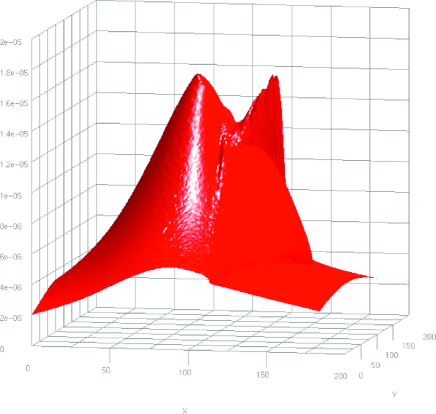
(a) $\Sigma$-map

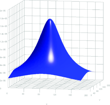
(b) King $\beta$-model

Figure 5: Comparison of the $\Sigma$-map data and the best-fit King $\beta$-model.The surface density $\Sigma$-map data reconstructed from X-ray imaging observations of the Bullet Cluster 1E0657-558, November 15, 2006 data release (Clowe et al., 2006b), is shown in red (a). The surface density $\Sigma$-map according to the best-fit King $\beta$-model (neglecting the subcluster) of Equation (34) is shown in blue (b). The best-fitting King $\beta$-model parameters are listed in Table 2.

King Model	Main Cluster	Subcluster
$\beta$	$0.803\pm 0.013$	…
$r_{c}$	$278.0\pm 6.8\ \mbox{kpc}$	…
$\rho_{0}$	$3.34\times 10^{5}\ M_{\odot}/\mbox{kpc}^{2}$	…
$M_{\rm gas}$	$3.87\times 10^{14}\ M_{\odot}$	$2.58\times 10^{13}\ M_{\odot}$
$r_{\rm out}$	$2620\ \mbox{kpc}$	…

Table 2: The best fit King $\beta$-model parameters.Using a nonlinear least-squares fitting routine, Equations (33) and (34) are fit to the $\Sigma$-map data for the main cluster (neglecting the subcluster). Results of our calculation for the main and subcluster mass, $M_{\rm gas}$, and cluster outer radial extent, $r_{\rm out}$ are listed below. The best-fit is shown in Figures 4 and 5b in blue, and may be compared to the data, in red.

We may now solve Equation (33) for the central density of the main cluster,

$$\rho_{0}=\frac{\Sigma_{0}}{\sqrt{\pi}r_{c}}\frac{\Gamma\left(\frac{3}{2}\beta\right)}{\Gamma\left(\frac{3\beta-1}{2}\right)}=3.34\times 10^{5}\ M_{\odot}/\mbox{kpc}^{2}.$$ (46)

The values of the parameters, $\beta$, $r_{c}$ and $\rho_{0}$ completely determine the King $\beta$-model for the density, $\rho(r)$, of Equation (21) of the main cluster X-ray gas. We provide a comparison of the full $\Sigma$-map data (Figure 5a, in red) with the result of the surface density $\Sigma$-map derived from the best-fit King $\beta$-model to the main cluster (Figure 5b, in blue).

Figure 6: The MOG mass scale, $M_{0}$, vs. $M_{\rm gas}$.A graphical calculation based on a power-law running of the MOG mass scale, $M_{0}$, depending on the total ICM gas mass, $M_{\rm gas}$, determined by the large ($>100$) galaxy cluster survey of Brownstein and Moffat (2006a). The computed values of $M_{\rm gas}$ and $M_{0}$ for the main and subcluster are listed in Table 3.

MOG	Main Cluster	Subcluster	Best-fit to $\kappa$-map
$M_{0}$	$1.02\times 10^{16}\ M_{\odot}$	$3.56\times 10^{15}\ M_{\odot}$	$3.07\times 10^{15}\ M_{\odot}$
$r_{0}$	$139.2\ \mbox{kpc}$	…	208.8 kpc
$\mathcal{G}_{\infty}$	$6.14$	…	3.82
$T$	$15.5\pm 3.9\ \mbox{keV}$	…	…

Table 3: MOG parameters.Results of calculation of the power-law running of the MOG mass scale, $M_{0}$, depending on the computed total cluster mass, $M_{\rm gas}$, according to the large ($>100$) galaxy cluster survey of Brownstein and Moffat (2006a) for the main and subcluster (shown graphically in Figure 6), and the overall best-fit to the $\kappa$-map; and the results for the MOG range parameter, $r_{0}$. Results of the calculations for the asymptotic value of the dimensionless gravitational coupling, $\mathcal{G}_{\infty}$, and the calculated X-ray temperature of the unperturbed isothermal sphere for the main cluster, $T$, are listed.

Substituting Equations (43), (44) and (46) into Equation (23), we obtain the main cluster outer radial extent,

$$r_{\rm out}=2620\ \mbox{kpc},$$ (47)

the distance at which the density, $\rho(r_{\rm out})$, drops to $\approx 10^{-28}\,\mbox{g/cm}^{3}$, or 250 times the mean cosmological density of baryons. The total mass of the main cluster may be calculated by substituting Equations (43), (44) and (46) into Equation (24):

$$M_{\rm gas}=3.87\times 10^{14}\ M_{\odot}.$$ (48)

III.2 The Gravitational Coupling for the Main cluster

As discussed in Section II.1, in order to apply the MOG model of Equation (18) to the Bullet Cluster 1E0657-558, we must first generalize the spherically symmetric case by treating the subcluster as a perturbation. In the zeroth order approximation, we begin by neglecting the subcluster. According to the large ($>100$) galaxy cluster survey of Brownstein and Moffat (2006a), the MOG mass scale, $M_{0}$, is determined by a power-law, depending only on the computed total cluster mass, $M_{\rm gas}$:

$$M_{0}=(60.4\pm 4.1)\times 10^{14}\ M_{\odot}\left(\frac{M_{\rm gas}}{10^{14}M_{\odot}}\right)^{0.39\pm 0.10}.$$ (49)

Substituting the result of Equation (48) for the main cluster into Equation (49), we obtain

$$M_{0}=1.02\times 10^{16}\ M_{\odot},$$ (50)

and substituting the result of Equation (48) for $M$ and Equation (50) for the main cluster of Bullet Cluster 1E0657-558 into Equation (19), we obtain

$$\mathcal{G}_{\infty}=6.14.$$ (51)

From Brownstein and Moffat (2006a), the MOG range parameter, $r_{0}$, depends only on the computed outer radial extent, $r_{\rm out}$:

$$r_{0}= r_{\rm out}/10, r_{\rm out}\leq 650\,\mbox{kpc},$$ (52)

$$r_{0}= 139.2\,{\rm kpc}, r_{\rm out}>650\,\mbox{kpc},$$

from which we obtain

$$r_{0}=139.2\ \mbox{kpc},$$ (53)

for the main cluster.

The best-fitting King $\beta$-model parameters for the main cluster are listed in Table 2, and the MOG parameters for the main cluster are listed in Table 3. A plot of the dimensionless gravitational coupling of Equation (18) using the MOG parameter results of Equations (50) and (53) for the main cluster (neglecting the subcluster) is plotted in Figure 7a using a linear scale for the $r$-axis, and in Figure 7b on a logarithmic scale for the $r$-axis.

(a) Linear Scale, $r$-axis.

(b) Logarithmic Scale, $r$-axis.

Figure 7: Plot of the dimensionless gravitational coupling, $\mathcal{G}(r)\equiv G(r)/G_{N}$, of Equation (18) vs. the distance, $r$, in kpc.Shown in linear scale for the $r$-axis, (a), and in logarithmic scale, (b). J2000 and map (x,y) coordinates of the MOG center ($R\equiv 0\ \mbox{kpc}$) are listed in Table 1, and located with respect to the $\Sigma$-map and $\kappa$-map in Figures 3 and 12, respectively. The running gravitational coupling, $\mathcal{G}(r)$, shown here, corresponds to our best-fit to the $\kappa$-map, listed in Table 3.

III.3 The Cylindrical Mass Profile

Figure 8: Cylindrical mass profileThe surface density $\Sigma$-map reconstructed from X-ray image observations of the Bullet Cluster 1E0657-558, November 15, 2006 data release (Clowe et al., 2006b) is integrated about the main cluster $\Sigma$-map peak ($R\equiv 0$), shown in solid red. The cylindrical mass profile derived from the best-fit King $\beta$-model is shown in short-dashed blue, demonstrating a good agreement with the data. The long-dash magenta line is the result of the galaxy subtraction of Equations (78) and (79). The lack of galactic mass in the vicinity of the main cluster $\Sigma$-map peak at $R=0$ is due to the merger. The dash-dot black line is the result of the dark matter subtraction of Equation (83). The dark matter dominates the ICM cluster gas by a factor $>3$. J2000 and map (x,y) coordinates are listed in Table 1. The best-fitting King $\beta$-model parameters are listed in Table 2.

$\Sigma(x,y)$ is an integrated density along the line-of-sight, $z$, as shown in Equation (36). By summing the $\Sigma$-map pixel-by-pixel, starting from the center of the main cluster $\Sigma$-map peak, one is performing an integration of the surface density, yielding the mass,

$$M(R)=\int_{0}^{R}\Sigma(R^{\prime})R^{\prime}dR^{\prime},$$ (54)

enclosed by concentric cylinders of radius, $R=\sqrt{x^{2}+y^{2}}$. We performed such a sum over the $\Sigma$-map data, and compared the result to the best-fit King $\beta$-model derived in Section III.1, with the parameters listed in Table 2. The results are shown in Figure 8. The fact that the data and model are in good agreement provides evidence that the King $\beta$-model is valid in all directions from the main cluster $\Sigma$-map peak, and not just on the straight line connecting the peak to the main cD, where the fit was performed. The model deviates slightly from the data, underpredicting $M(R)$ for $R>350\ \mbox{kpc}$, which may be explained by the subcluster (which is included in the data, but not the model). The integrated mass profile arising from the dark matter analysis of the $\kappa$-map of Equation (83) is shown for comparison on the same figure.

The ratio of dark matter to ICM gas for the main cluster is $>3$, which is significantly less than the average cosmological ratio of 5.68 discussed in Section I.1, whereas one should expect the highest mass to light ratios from large, hot, luminous galaxy clusters, and the Bullet Cluster 1E0657-558 is certainly one of the largest and hottest.

III.4 The Isothermal Spherical Mass Profile

For a spherical system in hydrostatic equilibrium, the structure equation can be derived from the collisionless Boltzmann equation

$$\frac{d}{dr}(\rho(r)\sigma_{r}^{2})+\frac{2\rho(r)}{r}\left(\sigma_{r}^{2}-\sigma_{\theta,\phi}^{2}\right)=-\rho(r)\frac{d\Phi(r)}{dr},$$ (55)

where $\Phi(r)$ is the gravitational potential for a point source, $\sigma_{r}$ and $\sigma_{\theta,\phi}$ are mass-weighted velocity dispersions in the radial ($r$) and tangential ($\theta,\phi$) directions, respectively. For an isotropic system,

$$\sigma_{r}=\sigma_{\theta,\phi}.$$ (56)

The pressure profile, $P(r)$, can be related to these quantities by

$$P(r)=\sigma_{r}^{2}\rho(r).$$ (57)

Combining equations (55), (56) and (57), the result for the isotropic sphere is

$$\frac{dP(r)}{dr}=-\rho(r)\frac{d\Phi(r)}{dr}.$$ (58)

For a gas sphere with temperature profile, $T(r)$, the velocity dispersion becomes

$$\sigma_{r}^{2}=\frac{kT(r)}{\mu_{A}m_{p}},$$ (59)

where $k$ is Boltzmann’s constant, $\mu_{A}\approx 0.609$ is the mean atomic weight and $m_{p}$ is the proton mass. We may now substitute equations (57) and (59) into equation (58) to obtain

$$\frac{d}{dr}\left(\frac{kT(r)}{\mu_{A}m_{p}}\rho(r)\right)=-\rho(r)\frac{d\Phi(r)}{dr}.$$ (60)

Performing the differentiation on the left-hand side of equation (58), we may solve for the gravitational acceleration:

$$a(r) \equiv -\frac{d\Phi(r)}{dr}$$ (61)

$$= \frac{kT(r)}{\mu_{A}m_{p}r}\left[\frac{d\ln(\rho(r))}{d\ln(r)}+\frac{d\ln(T(r))}{d\ln(r)}\right].$$

For the isothermal isotropic gas sphere, the temperature derivative on the right-hand side of equation (61) vanishes and the remaining derivative can be evaluated using the $\beta$-model of equation (21):

$$a(r)=-\frac{3\beta kT}{\mu_{A}m_{p}}\left(\frac{r}{r^{2}+r_{c}^{2}}\right).$$ (62)

Figure 9: The spherically integrated mass profile of the main cluster ICM gas.The mass profile integrated King $\beta$-model, $M_{\rm gas}(r)$, in from the $\Sigma$-map peak, is shown in long-dashed red. derived from the surface density $\Sigma$-map data reconstructed from X-ray imaging observations of the Bullet Cluster 1E0657-558, November 15, 2006 data release (Clowe et al., 2006b). The surface density $\Sigma$-map according to the best-fit King $\beta$-model (neglecting the subcluster) of Equation (34) is shown in black (with uncertainty). The Newtonian dynamical mass (the dark matter paradigm) is shown in short-dashed blue. All masses are presented in units of $M_{\odot}$, and distances, $r$, in kpc. The strong correspondence between the data (red) and the MOG fit (black) across distance scales in the cluster from tens to thousands of kpc. is significant. This is the first evidence that the X-ray imaging data for the cluster is behaving similar to the large ($>100$) galaxy cluster survey of Brownstein and Moffat (2006a). J2000 and map (x,y) coordinates are listed in Table 1. The best-fitting King $\beta$-model parameters are listed in Table 2. The best-fitting MOG parameters are listed in Table 3.

The dynamical mass in Newton’s theory of gravitation can be obtained as a function of radial position by replacing the gravitational acceleration with Newton’s Law:

$$a_{\rm N}(r)=-\frac{G_{N}M(r)}{r^{2}},$$ (63)

so that equation (61) can be rewritten as

$$M_{\rm N}(r)=-\frac{r}{G_{N}}\frac{kT}{\mu_{A}m_{p}}\left[\frac{d\ln(\rho(r))}{d\ln(r)}+\frac{d\ln(T(r))}{d\ln(r)}\right],$$ (64)

and the isothermal $\beta$-model result of equation (62) can be rewritten as

$$M_{\rm N}(r)=\frac{3\beta kT}{\mu_{A}m_{p}G_{N}}\left(\frac{r^{3}}{r^{2}+r_{c}^{2}}\right).$$ (65)

Similarly, the dynamical mass in MOG can be obtained as a function of radial position by substituting the MOG gravitational acceleration law (Moffat, 2005, 2006b; Brownstein and Moffat, 2006b, a)

$$a(r)=-\frac{G(r)M}{r^{2}},$$ (66)

so that our result for the isothermal $\beta$-model becomes

$$M_{\rm MOG}(r)=\frac{3\beta kT}{\mu_{A}m_{p}G(r)}\left(\frac{r^{3}}{r^{2}+r_{c}^{2}}\right).$$ (67)

We can express this result as a scaled version of equation (64) or the isothermal case of equation (65):

$$M_{\rm MOG}(r) = \frac{M_{\rm N}(r)}{\mathcal{G}(r)}$$ (68)

$$= \biggl{\{}1+\sqrt{\frac{M_{0}}{M_{\rm MOG}(r)}}\biggl{[}1-\exp(-r/r_{0})\biggl{(}1+\frac{r}{r_{0}}\biggr{)}\biggr{]}\biggr{\}}^{-1}M_{\rm N}(r),$$

where we have substituted Equation (18) for $\mathcal{G}(r)$. Equation (68) may be solved explicitly for $M_{\rm MOG}(r)$ by squaring both sides and determing the positive root of the quadratic equation.

Year	Source - Theory or Experiment	$T\ (\mbox{keV})$	% error
2007	MOG PredictionExperiment 012	$15.5\pm 3.9$
2002	accepted experimental value	$14.8^{+1.7}_{-1.2}$	$\phantom{X1}4.5$
1999	ASCA+ROSAT fit	$14.5^{+2.0}_{1.7}$	$\phantom{X1}6.5$
1998	ASCA fit	$17.4\pm 2.5$	$\phantom{X}12.3$

Table 4: The MOG best-fit temperature is consistent with the experimental values for the main cluster isothermal temperature, the 1999 ASCA+ROSAT fit, and the 1998 ASCA fit (Markevitch et al., 2002).

The scaling of the Newtonian dynamical mass by $\mathcal{G}(r)$ according to Equation (68) solved the dark matter problem for the galaxy clusters of the $>100$ galaxy cluster survey of Brownstein and Moffat (2006a). The unperturbed Bullet Cluster 1E0657-558 is no exception! In Figure 9, we plotted the MOG and the Newtonian dynamical masses, $M_{\rm MOG}(r)$ and $M_{\rm N}(r)$, respectively, and compared it to the spherically integrated best-fit King $\beta$-model for the main cluster gas mass of Equations (21) and (22) using the parameters listed in Table 2. The MOG temperature prediction due to the best-fit is listed in Table 4 and compared to experimental values.

As shown in Figure 9, across the range of the $r$-axis, and throughout the radial extent of the Bullet Cluster 1E0657-558, the $1\sigma$ correlation between the gas mass, $M(r)$ and the MOG dynamical mass, $M_{\rm MOG}(r)$, provides excellent agreement between theory and experiment. The same cannot be said of any theory of dark matter in which the X-ray surface density map is negligible in relation to the DM density. So dark matter makes no prediction for the isothermal temperature, which has been measured to reasonable precision for many clusters, but simply “accounts for missing mass.” Since there is no mysterious missing mass in MOG, the prediction should be taken seriously as direct confirmation of the theory, or at least as hard evidence for MOG.

III.5 The Subcluster Subtraction

Figure 10: The subcluster subtracted surface density $\Sigma$-mapMain cluster and subcluster $\kappa$-map observed peaks (local maxima) and $\Sigma$-map observed peaks are shown for comparison. The central dominant (cD) galaxy of the main cluster, the brightest cluster galaxy (BCG) of the subcluster, and the MOG predicted gravitational center are shown. The colourscale is set to agree with Figure 3 for comparison. J2000 and map (x,y) coordinates are listed in Table 1.

Provided the surface density $\Sigma$-map derived from the best-fit King $\beta$-model of Equation (34) is sufficiently close to the $\Sigma$-map data (consider Figures 4 and 5) then the difference between the data and the $\beta$-model is the surface density $\Sigma$-map due to the subcluster. Our subcluster subtraction, shown in Figures 10 and 11a, is based upon a high precision ($\chi^{2}<0.2$) best-fit King $\beta$-model to the main cluster, which agrees with the main cluster surface mass $\Sigma$-map (data) within 1% everywhere and to a mean uncertainy of 0.8%. The subcluster subtraction is accurate down to $\rho=10^{-28}\ \mbox{g}/\mbox{cm}^{3}\sim 563.2\ M_{\odot}/\mbox{pc}^{3}$ baryonic background density. After subtraction, the subcluster $\Sigma$-map peak takes a value of $1.30\times 10^{8}\ M_{\odot}/\mbox{kpc}^{2}$, whereas the full $\Sigma$-map has a value of $2.32\times 10^{8}\ M_{\odot}/\mbox{kpc}^{2}$ at the subcluster $\Sigma$-map peak. Thus the subcluster (at its most dense position) provides only $\approx 56\%$ of the X-ray ICM, the rest is due to the extended distribution of the main cluster. The subcluster subtraction surface density $\Sigma$-map shown in Figure 10 uses the same colorscale as the full $\Sigma$-map shown in Figure 3, for comparison. Figure 11 is a stereogram of the subcluster subtracted surface density $\Sigma$-map and the subcluster superposed onto the surface density $\Sigma$-map of the best-fit King $\beta$-model to the main cluster. There is an odd X-ray bulge in Figures 10 and 11b which may be an artifact of the subtraction, or perhaps evidence of an as yet unidentified component.

Since the outer radial extent of the subluster gas is less than 400 kpc, the $\Sigma$-map completely contains all of the subcluster gas mass. By summing the subcluster subtracted $\Sigma$-map pixel-by-pixel over the entire $\Sigma$-map peak, one is performing an integration of the surface density, yielding the total subcluster mass. We performed such a sum over the subcluster subtracted $\Sigma$-map data, obtaining

$$M_{\rm gas}=2.58\times 10^{13}\ M_{\odot},$$ (69)

for the mass of the subcluster gas, which is less than 6.7% of the mass of main cluster gas (the best-fitting King $\beta$-model parameters are listed in Table 2.) This justifies our initial assumption that the subcluster may be treated as a perturbation in order to fit the main cluster to the King $\beta$-model. Our subsequent analysis of the thermal profile confirms that the main cluster X-ray temperature is nearly isothermal, lending further support to the validity of the King $\beta$-model.

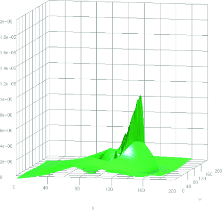
(a) The subcluster subtracted surface density $\Sigma$-map

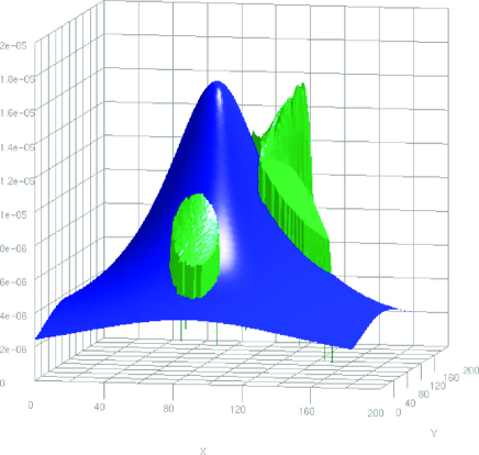
(b) The subcluster subtracted $\Sigma$-map superposed onto the best-fit King $\beta$-model of the main cluster. Note the odd X-ray Bulge, here, and in Figure 10.

Figure 11: The subcluster subtracted surface density $\Sigma$-map.The blue surface represents the $\Sigma$-map due to the integrated (line-of-sight) King $\beta$-model fit to main cluster (as shown in blue in Figure 5b). The green surface is the contribution to the $\Sigma$-map from the subcluster (as calculated from our model). J2000 and map (x,y) coordinates are listed in Table 1. The best-fitting King $\beta$-model parameters are listed in Table 2.

We may now calculate the MOG mass scale, $M_{0}$, of the subcluster by substituting the subcluster gas mass, $M_{\rm gas}$, of Equation (69) into the power-law relation of Equation (49), yielding,

$$M_{0}=3.56\times 10^{15}\ M_{\odot},$$ (70)

as shown in Figure 6. The computed values of $M_{\rm gas}$ and $M_{0}$ for the main and subcluster are listed in Table 3.

IV The Convergence Map from Lensing Analysis

IV.1 The $\kappa$-Map

Figure 12: The surface density $\kappa$-map reconstructed from strong and weak gravitational lensing. Main cluster and subcluster of the Bullet Cluster 1E0657-558, November 15, 2006 data release $\kappa$-map (Clowe et al., 2006b) observed peaks (local maxima) and $\Sigma$-map observed peaks are shown for comparison. The central dominant (cD) galaxy of the main cluster, the brightest cluster galaxy (BCG) of the subcluster, and the MOG predicted gravitational center are shown. J2000 and map (x,y) coordinates are listed in Table 1.

As tempting as it is to see the convergence $\kappa$-map of Figure 12 – a false color image of the strong and weak gravitational lensing reconstruction (Clowe et al., 2006a; Bradač et al., 2006; Clowe et al., 2006c) – as a photograph of the “curvature” around the Bullet Cluster 1E0657-558, it is actually a reconstruction of all of the bending of light over the entire distance from the lensing event source toward the Hubble Space Telescope. The source of the $\kappa$-map is $\propto\int G_{N}\rho(r)$, along the line-of-site, as in Equation (35), $\propto G(r)\int\rho(r)$ as in Equation (39), or $\propto\int G(r)\rho(r)$ as in Equation (41). For the Bullet Cluster 1E0657-558, we are looking along a line-of-sight which is at least as long as indicated by a redshift of $z=0.296$ (Gpc scale). The sources of the lensing events are in a large neighbourhood of redshifts, an estimated $z=0.85\pm 0.15$. This fantastic scale (several Gpc) is naturally far in excess of the distance scales involved in the X-ray imaging surface density $\Sigma$-map. It is an accumulated effect, but only over the range of the X-ray source – as much as 2.2 Mpc. A comparison of these two scales indicates that the distance scales within the $\Sigma$-map are $10^{-3}$ below the Gpc’s scale of the $\kappa$-map.

Preliminary comments on the November 15, 2006 data release (Clowe et al., 2006b):

• The conclusion of Clowe et al. (2006a); Bradač et al. (2006), that the $\kappa$-map shows direct evidence for the existence of dark matter may be premature. Until dark matter has been detected in the lab, it remains an open question whether a modified gravity theory, such as MOG, can account for the $\kappa$-map without nonbaryonic dark matter. MOG, due to the varying gravitational coupling, Equation (18), gives the Newtonian $1/r^{2}$ gravitational force law a considerable boost – “extra gravity” as much as $\mathcal{G}_{\infty}\approx 6$ for the Bullet Cluster 1E0657-558.

• It may be feasible that the mysterious plateau in the north-east corner of the $\kappa$-map is from some distribution of mass unrelated to the Bullet Cluster 1E0657-558. This “background curvature” contribution to the $\kappa$-map is one part of the uncertainty in the reconstruction. The second, dominant source of uncertainty certainly must be the estimate of the angular diameter distances between the source of the lensing event and the Bullet Cluster 1E0657-558, as shown in Equation (37).

We have completed a large ($>100$) galaxy cluster survey in Brownstein and Moffat (2006a) that provides a statistically significant answer to the question of how much dark matter is expected. The relative abundance across the scales of the X-ray clusters would imply that the $\kappa$-map should peak at $\sim 1.0$ as opposed to the November 15, 2006 data release (Clowe et al., 2006b), which peaks at a value of $\kappa\approx 0.38$ for the main cluster $\kappa$-map peak.

Where is the missing dark matter?

The dark matter paradigm cannot statistically account for such an observation without resorting to further ad-hoc explanation, so the question of “missing matter” may be irrelevant. The problem of “extra gravity” due to MOG may be a step in the right direction, with our solution as the subject of the next section.

IV.2 The MOG Solution

The MOG $\kappa$-model we have developed in Equations (41) and (42) can now be applied to the Bullet Cluster 1E0657-558. In order to model the $\kappa$-map, shown in Figures 12 and 14a, in MOG, we must integrate the product of the dimensionless gravitational coupling, $\mathcal{G}(r)$ of Equation (18) with the mass density, $\rho(r)$, over the volume of the Bullet Cluster 1E0657-558. As discussed in Section III.3, we may integrate the surface density $\Sigma$-map data according to Equation (54) to obtain the integrated cluster gas mass about concentric cylinders centered about $R=0$. However, what we require in the calculation of the $\mathcal{G}(r)$ of Equation (18) is the integrated mass about concentric spheres,

$$M(r)=\int_{0}^{2\pi}d\theta\int_{0}^{\pi}\sin\phi\,d\phi\int_{0}^{r}{r^{\prime}}^{2}d{r^{\prime}}\rho({r^{\prime}},\theta,\phi).$$ (71)

The calculation of $M(r)$ using Equation (71) is non-trivial, and we proceed by making a suitable approximation to the density, $\rho(r)$. As discussed in Section II.1, we may apply a sequence of approximations to develop a MOG solution.

$0^{\rm th}$-order approximation:

We have obtained the spherically integrated best-fit King $\beta$-model for the main cluster gas mass of Equations (21) and (22) using the parameters listed in Table 2. By neglecting the subcluster, we have generated a base-line solution similar to every other spherically symmetric galaxy cluster. The result of substituting the spherically symmetric King $\beta$-model mass profile of Equation (22) into Equation (18) is shown in Figure 7 for the dimensionless gravitational coupling, $\mathcal{G}(r)$. We obtain a zeroth order, spherically symmetric approximation to the $\kappa$-map by substituting $\rho(r)$ and $\mathcal{G}(r)$ into Equations (41) and (42) and integrating over the volume.

MOG Center:

Treat the subcluster as a perturbation, and shift the origin of $\mathcal{G}(r)$ toward the subcluster (toward the center-of-mass of the system). In this approximation, we continue to use the spherically integrated best-fit King $\beta$-model for the main cluster gas mass of Equations (21) and (22) using the parameters listed in Table 2, but we allow the subcluster to perturb (shift) the origin of $\mathcal{G}(r)$ toward the true center-of-mass of the system. The integrals of Equations (41) and (42) become nontrivial as the integrand is no longer spherically symmetric. We were able to obtain a full numerical integration, but the computation proved to be too time consuming ($\sim 70,000$ numerical integrations to cover the $185\times 185\ \mbox{pixel}^{2}$) to treat by means of a nonlinear least-squares fitting routine.

Projective approximation: Approximate $M(r)$ with the concentric cylinder mass, $M(R)$ of Equation (54), calculated directly from the $\Sigma$-map, where the pixel-by-pixel sum proceeds from the MOG center. This is a poor approximation for small $R$ (few pixels), but becomes very good for large $R$ (many pixels), as can be seen by comparing Figures 8 and 9. The cylindrical mass, $M(R)$, can be computed directly from the $\Sigma$-map data using Equation (54) without the need of a King $\beta$-model.

Isothermal $\beta$-model approximation:

Treat the subcluster as a perturbation, and utilize the isothermal $\beta$-model of Equation (68) to approximate $M(r)$ and shift that toward the subcluster (toward the MOG center). This is a fully analytic expression, allowing ease of integration and an iterative fitting routine.

We will base our analysis on our best-fit determined by the isothermal $\beta$-model approximation of Equation (68), with $\mathcal{G}(r)$ located at the MOG center, a distance away from the main cluster $\Sigma$-map peak toward the subcluster $\Sigma$-map peak. Since the dimensionless gravitational coupling, $\mathcal{G}(r)$, of Equation (18) depends on $M(r)$, and the isothermal $\beta$-model of Equation (68) depends on $\mathcal{G}(r)$, we must solve the system simultaneously. Let us rewrite Equation (18)

$$\mathcal{G}(r)=1+\sqrt{\frac{\xi(r)}{M(r)}},$$ (72)

where

$$\xi(r)=M_{0}\left\{1-\exp\left(-\frac{r}{r_{0}}\right)\left(1+\frac{r}{r_{0}}\right)\right\}^{2}.$$ (73)

We may solve Equation (72) for

$$M(r)={\frac{\xi(r)}{\left(\mathcal{G}(r)-1\right)^{2}}},$$ (74)

and equate this to the isothermal $\beta$-model of Equation (68):

$${\frac{\xi(r)}{\left(\mathcal{G}(r)-1\right)^{2}}}=\frac{M_{\rm N}(r)}{\mathcal{G}(r)},$$ (75)

and we may solve the quadratic equation for

$$\mathcal{G}(r)=1+\frac{\xi(r)}{2M_{\rm N}(r)}\left\{1+\sqrt{\frac{4M_{\rm N}(r)}{\xi(r)}+1}\right\},$$ (76)

where $M_{\rm N}$ is the isothermal $\beta$-model Newtonian dynamic mass of Equation (65). The result of Equation (76) is a fully analytic function, as opposed to a hypergeometric integral, and may be easily computed across the full $\kappa$-map. There was a noticeable parameter degeneracy in choosing the MOG center, the best-fit corresponded to a distance of 140 kpc away from the main cluster $\Sigma$-map peak toward the subcluster $\Sigma$-map peak. This is reasonable since the $\Sigma$-map and $\kappa$-map data are two-dimensional “surface projections”, due to the line-of-sight integral. The full simulation was run iteratively over a range of positions for the MOG center, while covarying the MOG parameters, $M_{0}$ and $r_{0}$, the MOG mass scale and MOG range parameter, respectively. This yielded a best-fit MOG model for the dimensionless gravitational coupling, $\mathcal{G}(r)$ of Equation (18), where $r$ is the distance from the MOG center, as listed in Table 3. Our best-fit to the $\kappa$-map corresponds to the MOG $\kappa$-model of Equations (41) and (42). The best-fit location of the MOG center is provided on the $\Sigma$-map in Figure 3, and the coordinates are listed in Table 1.

We show a 3D visualization of the convergence $\kappa$-map data in Figure 14a. The $0^{\rm th}$-order approximation result, rescaled is shown in Figure 14b. The twin humps at the peaks of our prediction will be a generic prediction for any spherically symmetric galaxy cluster (non-mergers). The best-fit MOG $\kappa$-model is shown in Figure 14c along the line connecting the MOG center to the main cluster $\kappa$-map peak. We show a 3D visualization of the full convergence $\kappa$-map model in Figure 14d.

IV.3 Including the Galaxies

Figure 13: The galaxy surface density $\Sigma$-map prediction.The prediction of the $\Sigma$-map due to the galaxies as computed by the difference between the $\kappa$-map and our MOG $\kappa$-model, scaled as surface mass density according to Equation (78). $\Sigma$-map and $\kappa$-map observed peaks are shown for comparison. The central dominant (cD) galaxy of the main cluster, the brightest cluster galaxy (BCG) of the subcluster, and the MOG predicted gravitational center are shown. J2000 and map (x,y) coordinates are listed in Table 1. Component masses (integrated within a 100 kpc radius aperture) for the main and subcluster, the MOG center and the total predicted baryonic mass, $M_{\rm bary}$, for the Bullet Cluster 1E0657-558 are shown in Table 5.

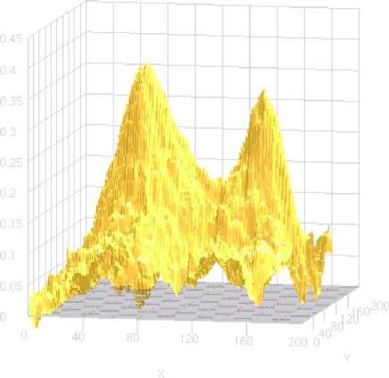
(a) 3D visualization of the $\kappa$-map November 15, 2006 data release (Clowe et al., 2006b)

(b) $0^{\rm th}$-order approximation – neglecting the subcluster

(c) Best-fit $\kappa$-model

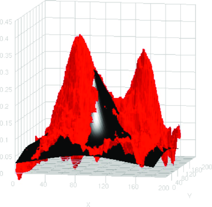
(d) 3D visualization of the best-fit $\kappa$-model

Figure 14: The convergence $\kappa$-map November 15, 2006 data release (Clowe et al., 2006b) and our $\kappa$-models.The best-fit MOG $\kappa$-model is shown in solid black in Figures 14b, 14c and 14d. The convergence $\kappa$-map November 15, 2006 data release (Clowe et al., 2006b) is shown as Figure 14a and in red in Figures 14b, 14c and 14d. The scaled $\Sigma$-map, $\Sigma(x,y)/\Sigma_{c}$ data is shown in short-dashed green, also shown in Figure 4.

In considering the MOG $\kappa$-model resulting from the $0^{\rm th}$-order approximation, as shown in Figure 14b, it is tempting to try to explain the entire convergence $\kappa$-map by the X-ray gas mass, just by shifting the solid-black line to the left by $\sim 200$ kpc, but then there would be no way to explain the subcluster $\kappa$-map peak. We next proceed to account for the effect of the subcluster on the dimensionless gravitational coupling, $\mathcal{G}(r)$, of MOG, as shown in the best-fit $\kappa$-model of Figures 14c and 14d. Remarkably, as the MOG center is separated from the main cluster $\Sigma$-map peak, say due to the gravitational effect of the subcluster, the centroid naturally shifts toward the $\kappa$-map peak, and the predicted height of the $\kappa$-map drops. Let us take the difference between the $\kappa$-map data and our best-fit $\kappa$-model, to see if there is any “missing mass”. We hypothesize that the difference can be explained by including the galaxies,

$$\kappa(x,y)=\frac{{\bar{\Sigma}}(x,y)+{\bar{\Sigma}}_{\rm galax}(x,y)}{\Sigma_{c}},$$ (77)

where $\bar{\Sigma}$ is the weighted surface mass density of Equation (42), and the best-fit $\kappa$-model of ${\bar{\Sigma}}/\Sigma_{c}$ is derived from Equations (41) and (42). Therefore, the galaxies contribute a “measurable” surface mass density,

$$\Sigma_{\rm galax}(x,y)\approx\frac{\kappa(x,y)\Sigma_{c}-{\bar{\Sigma}}(x,y)}{\mathcal{G}(x,y)},$$ (78)

where $\mathcal{G}(x,y)$ corresponds to the best-fit model of Equation (18) listed in Table 3. The result of the galaxy subtraction of Equation (78) is shown in Figure 13. Now we may interpret Figure 14d as the total convergence $\kappa$-map where the black surface is the contribution from the weighted surface density of the ICM gas, ${\bar{\Sigma}}/\Sigma_{c}$, and the red surface is the remainder of the $\kappa$-map due to the contribution of the weighted surface density of the galaxies, ${\bar{\Sigma}}_{\rm galax}/\Sigma_{c}$. We may calculate the total mass of the galaxies,

$$M_{\rm galax}=\int\Sigma_{\rm galax}(x^{\prime},y^{\prime})dx^{\prime}\,dy^{\prime}.$$ (79)

Component	Main cluster	Subcluster	Central ICM	Total
$M_{\rm gas}$	$7.0\times 10^{12}\ M_{\odot}$	$5.8\times 10^{12}\ M_{\odot}$	$6.3\times 10^{12}\ M_{\odot}$	$2.2\times 10^{14}\ M_{\odot}$
$M_{\rm galax}$	$1.8\times 10^{12}\ M_{\odot}$	$3.1\times 10^{12}\ M_{\odot}$	$2.4\times 10^{10}\ M_{\odot}$	$3.8\times 10^{13}\ M_{\odot}$
$M_{\rm bary}$	$8.8\times 10^{12}\ M_{\odot}$	$9.0\times 10^{12}\ M_{\odot}$	$4.9\times 10^{12}\ M_{\odot}$	$2.6\times 10^{14}\ M_{\odot}$
$M_{\rm DM}$	$2.1\times 10^{13}\ M_{\odot}$	$1.7\times 10^{13}\ M_{\odot}$	$1.4\times 10^{13}\ M_{\odot}$	$6.8\times 10^{14}\ M_{\odot}$
$M_{\rm galax}/M_{\rm gas}$	$26\%$	$53\%$	$0.4\%$	$17\%$
$M_{\rm gas}/M_{\rm DM}$	$33\%$	$34\%$	$45\%$	$32\%$

Table 5: Summary of component mass predictions.Component masses (integrated within a 100 kpc radius aperture) for the main and subcluster and the MOG center. The total predicted mass for the Bullet Cluster 1E0657-558 is integrated over the full $\Sigma$-map.

We were able to perform the integration within a 100 kpc radius aperture about the main cluster cD and subcluster BCG, separately, the results of which are listed in Table 5, where they are compared with the upper limits on galaxy masses set by HST observations. If the hypothesis that the predicted $M_{\rm galax}$ is below the bound set by HST observations is true, then it follows that

$$M_{\rm bary}=M_{\rm gas}+M_{\rm galax},$$ (80)

requires no addition of non-baryonic dark matter. The results of our best-fit for $M_{\rm gas}$, $M_{\rm galax}$ and $M_{\rm bary}$ of Equation (80) are listed in Table 5.

IV.4 Dark Matter

From the alternative point-of-view, dark matter is hypothesized to account for all of the “missing mass” which results in applying Newton/Einstein gravity. This means, for the November 15, 2006 data release (Clowe et al., 2006a; Bradač et al., 2006; Clowe et al., 2006c, b), that the “detected” dark matter must contribute a surface mass density,

$$\Sigma_{\rm DM}(x,y)\approx\kappa(x,y)\Sigma_{c}-\Sigma(x,y),$$ (81)

with an associated total mass,

$$M_{\rm DM}=\int\Sigma_{\rm DM}(x^{\prime},y^{\prime})dx^{\prime}\,dy^{\prime}.$$ (82)

The integral of Equation (82) becomes trivial upon substitution of Equation (81):

$$M_{\rm DM}=\Sigma_{c}\int\kappa(x^{\prime},y^{\prime})dx^{\prime}\,dy^{\prime}-\int\Sigma(x^{\prime},y^{\prime})dx^{\prime}\,dy^{\prime}$$ (83)

where we have neglected $M_{\rm galax}$ in Equation (83), because as is usually argued, the contribution from the galaxies in the dark matter paradigm is $\leq 1$ – $4\%$ of $M_{\rm total}$. The calculation of $M_{\rm DM}$ in Equation (83) was performed by a pixel-by-pixel sum over the convergence $\kappa$-map data and surface density $\Sigma$-map data, within a 100 kpc radius aperture around the main and subcluster $\kappa$-map peaks, respectively. The result of our computation is included in Table 5. We emphasize, here, that for each of the main cluster, subcluster and total $\Sigma$-map, our results of Table 5 indicate that

$$M_{\rm bary}=M_{\rm gas}+M_{\rm galax}\ll M_{\rm DM}$$ (84)

implying that we have successfully put Bullet Cluster 1E0657-558 on a lean diet! This seems to us to be a proper use of Occam’s razor. The mass ratios, $M_{\rm galax}/M_{\rm gas}$, for the main and subcluster and central ICM are shown at the bottom of Table 5. The result of $M_{\rm galax}/M_{\rm gas}\approx 0.4\%$ in the central ICM is due to the excellent fit in MOG across the hundreds of kpc separating the main and subcluster. The dark matter result of $M_{\rm gas}/M_{\rm DM}\approx 45\%$ in the central ICM implies that the evolutionary scenario does not lead to a spatial dissociation between the dark matter and the ICM gas, which indicates that the merger is ongoing. In contrast, the MOG result shows a true dissociation between the galaxies and the ICM gas as required by the evolutionary scenario. The baryon to dark matter fraction over the full $\Sigma$-map is $32\%$, which is significantly higher than the $\Lambda$-CDM cosmological baryon mass-fraction of $17^{+1.9}_{-1.2}\%$ (Spergel et al., 2007). The distribution of mass predicted by MOG vs. the dark matter paradigm is shown in Figure 15.

(a) Scaled surface density for the MOG predicted galaxies, $\Sigma_{\rm galax}/\Sigma_{c}$, and the MOG predicted visible baryons, $\Sigma_{\rm bary}/\Sigma_{c}$, compared to the ICM gas.

(b) Scaled surface density of dark matter, $\Sigma_{\rm DM}/\Sigma_{c}$, compared to ICM gas.

Figure 15: Plot of the scaled surface density $\Sigma/\Sigma_{c}$ along the line connecting the main cluster $\Sigma$-map peak with the main cD.In Figure 15a, the prediction of Equation (78) for the galaxies is shown in long-dashed magenta, and the prediction of Equation (80) for the visible baryonic mass is shown in solid brown. The calculation of Equation (81) for dark matter is shown in Figure 15b in dash-dot black. The ICM gas distribution inferred from the $\Sigma$-map data is shown in short-dashed green on each plot.

V Conclusions

The modified gravity (MOG) theory provides a fit to the $\kappa$-map of the November 15, 2006 data release (Clowe et al., 2006b). The model, derived purely from the X-ray imaging $\Sigma$-map observations combined with the galaxy $\Sigma$-map predicted by MOG, accounts for the $\kappa$-map peak amplitudes and their spatial dissociation without the introduction of nonbaryonic dark matter.

The question of the internal degrees of freedom in MOG has to be further investigated. It would be desirable to derive a theoretical prediction from the MOG field equations that fits the empirically determined mass and distance scales in Figure 2.

It could be argued that any modified theory designed to solve the dark matter conundrum, such as MOND or MOG, has less freedom than dark matter. So the important question to resolve is precisely how much freedom the MOG solution has. On one hand we said, definitely, that there was no freedom in choosing the pair of $M_{0}$ and $r_{0}$ for the main cluster since it was well described by an isothermal sphere, to an excellent approximation. We further argued that the subcluster was (per mass) a small perturbation to the ICM. But if MOG has more freedom than MOND, but less freedom than Dark Matter, then what is the additional degree of freedom that enters the Bullet Cluster observations?

The question is resolved in that there is a physical degree of freedom due to a lack of spherical symmetry in the Bullet Cluster, and whence the galaxies sped outward, beyond the ICM gas clouds which lagged behind – effectively allowing the galaxies to climb out of the spherical minimum of the Newtonian core where MOG effects are small (inside the MOG range $r_{0}$) upwards along the divergence of the stress-energy tensor (Newtonian potential, if you prefer a simple choice) towards the far infrared region of large gravitational coupling, ${G}_{\infty}$.

In fact, the Bullet Cluster data results describe, to a remarkable precision, a simple King $\beta$-Model. Our analysis, with the result to the best-fit shown in Table 2, uniquely determines the mass profile $\rho(r)$ of Equation (21) used throughout our computations. We permitted only a single further degree of freedom to account for the fits of Figure 14c and the predictions of Figures 13 and 15; this was the location of the MOG center, where the gravitational coupling, $\mathcal{G}(0)\rightarrow 1$, is a minimum at the Newtonian core. Remarkably, the data did not permit a vanishing MOG center, with respect to the peak of the ICM gas $\rho(0)$. We have shown the location of the MOG center as determined by a numerical simulation of convergence map according to Equations (41) and (42) in each of Figures 3, 10, 12 and 13 and provided the coordinates in Table 1.

The surface density $\Sigma$-map derived from X-ray imaging observations is separable into the main cluster and the subcluster subtracted surface density $\Sigma$-map through a low $\chi^{2}$-fitting King $\beta$-model. Following the ($>100$) galaxy cluster survey of Brownstein and Moffat (2006a), we have derived a parameter-free (unique) prediction for the X-ray temperature of the Bullet Cluster 1E0657-558 which has already been experimentally confirmed. In Equations (41) and (42), we have derived a weighted surface mass density, $\bar{\Sigma}$, from the convergence $\kappa$-map which produced a best-fit model (Figures 14c and 14d and Table 3). We have computed the dark matter and the MOG predicted galaxies and baryons (Figure 15), and noted the tremendous predictive power of MOG as a means of utilizing strong and weak gravitational lensing to do galactic photometry – a powerful tool simply not provided by any candidate dark matter (Figure 13). The predictions for galaxy photometry will be the subject of future investigations in MOG, and the availability of weak and strong gravitational lensing surveys will prove invaluable in the future.

Although dark matter allows us to continue to use Einstein (weak-field) and Newtonian gravity theory, these theories may be misleading at astrophysical scales. By searching for dark matter, we may have arrived at a means to answer one of the most fundamental questions remaining in astrophysics and cosmology: How much matter (energy) is there in the Universe and how is it distributed? For the Bullet Cluster 1E0657-558, dark matter dominance is a ready answer, but in MOG we must answer the question with only the visible contribution of galaxies, ICM gas and gravity.