Signatures of Delayed Detonation, Asymmetry, and Electron Capture in the Mid-Infrared Spectra of Supernovae 2003hv and 2005df

Abstract

We present mid-infrared (5.2–15.2 µm) spectra of the Type Ia supernovae (SNe Ia) 2003hv and 2005df observed with the Spitzer Space Telescope. These are the first observed mid-infrared spectra of thermonuclear supernovae, and show strong emission from fine-structure lines of Ni, Co, S, and Ar. The detection of Ni emission in SN 2005df 135 days after the explosion provides direct observational evidence of high-density nuclear burning forming a significant amount of stable Ni in a Type Ia supernova. The observed emission line profiles in the SN 2005df spectrum indicate a chemically stratified ejecta structure. The Ar and Ni lines in SN 2005df are both shifted to the red relative to the Co emission, which appears to be nearly centered with respect to the rest frame of the host galaxy. The SN 2005df Ar lines also exhibit a two-pronged emission profile implying that the Ar emission deviates significantly from spherical symmetry. The observed Ar lines can be reproduced with either an almost circular ring-shaped geometry observed nearly edge-on, or a prolate ellipsoidal emission geometry with a central hole observed nearly pole-on. The spectrum of SN 2003hv also shows signs of asymmetry, exhibiting blueshifted [Co III] which matches the blueshift of [Fe II] lines in nearly coeval NIR spectra. Finally, local thermodynamic equilibrium abundance estimates for the yield of radioactive ⁵⁶Ni give $M_{{}^{56}Ni}\approx 0.5M_{\sun}$, for SN 2003hv, but only $M_{{}^{56}Ni}\approx 0.13$–$0.22M_{\sun}$ for the apparently subluminous SN 2005df, supporting the notion that the luminosity of SNe Ia is primarily a function of the radioactive ⁵⁶Ni yield.

The chemically stratified ejecta structure observed in SN 2005df matches the predictions of delayed-detonation (DD) models, but is entirely incompatible with current three-dimensional deflagration models. Furthermore the degree that this layering persists to the innermost regions of the supernova is difficult to explain even in a DD scenario, where the innermost ejecta are still the product of deflagration burning. Thus, while these results are roughly consistent with a delayed detonation, it is clear that a key piece of physics is still missing from our understanding of the earliest phases of SN Ia explosions.

1. Introduction

There is general agreement about the basic nature of Type Ia supernovae (SNe Ia): they are the thermonuclear explosion of degenerate white dwarfs (WDs), probably in some sort of close binary system undergoing some form of mass transfer, and exploding once a critical mass is reached, likely near the Chandrasekhar limit, at least for the majority of SN Ia events. (For reviews, see Branch 1998; Leibundgut 2001; Nomoto et al. 2003; Höflich et al. 2003.) Still, many of the details of this picture remain either unknown or are highly controversial. In particular, the initial conditions of the WD progenitor prior to thermonuclear runaway, and the dynamical propagation of the nuclear burning are both hotly debated topics of discussion.

The recent growth in the availability of infrared (IR) observations shows much promise in addressing these issues. Infrared spectroscopy has several fundamental advantages over UV/optical spectroscopy for work on SNe Ia. First, the strong spectral features in the IR are spread farther apart in wavelength, avoiding most of the strong line-blending issues that complicate the analysis of optical/UV observations. Consequently, kinematic information can be extracted directly from the observed line profiles without relying on a detailed spectral synthesis calculation. Second, IR lines tend to have a lower optical depth than UV/optical lines which, combined with the reduced line blending, greatly aids in the accurate measurement of abundances of iron-peak elements.

This is particularly true of ground-state transitions in the mid-infrared (MIR). For these low-excitation lines the effects of stimulated emission are very strong, dramatically reducing the optical depth. Thus, these lines can become optically thin quite rapidly, often while the electron densities are still well above the critical density for collisional de-excitation. As a result, relatively accurate (and temperature insensitive) abundance estimates can be made from MIR lines using just a local thermodynamic equilibrium (LTE) approximation. Finally, near-IR and mid-IR observations can be used to put strong constraints on the formation of molecules and dust in the cooling ejecta.

However, IR observations have one disadvantage. While the IR flux of SNe Ia is intrinsically fainter than in the optical, the foreground and background emission is usually much larger. In particular, foreground thermal emission precludes MIR spectroscopy of all but the very nearest extragalactic SNe Ia from the ground, and to date, IR spectroscopic observations of SNe Ia have been limited to the near-infrared (NIR). With the launch of the Spitzer Space Telescope (Werner et al., 2004), MIR spectroscopy is now possible, at least for nearby ($D\lesssim 25$ Mpc) SNe Ia. In this paper we present the first MIR spectra of SNe Ia, obtained with the Infrared Spectrograph (IRS; Houck et al., 2004) on the Spitzer Space Telescope: A low signal-to-noise ratio (S/N) spectrum of SN 2003hv and the first of two planned high S/N observations of SN 2005df. Both were obtained as part of the GO program of the Mid-Infrared Supernova Consortium (MISC).

In § 2 we describe the observations and data reduction, and the results are shown in § 3, including a detailed discussion of line identifications. In § 4 we analyze the observed emission-line profiles using synthetic line profiles from simple models of the emission distribution. In § 5, we use the observed nickel and cobalt line fluxes to infer abundances assuming LTE level populations, and make estimates for the optical depth and electron density. Finally, we discuss and summarize our results in § 6 and § 7.

2. Observations and Data Reduction

SN 2003hv was discovered at about 12.5 mag on 9.5 Sep 2003 (all dates UT) in NGC 1201 by Beutler & Li (2003), and classified as a SN Ia on 10.3 Sep. 2003 by Dressler et al. (2003), closely resembling SN 1994D two days after maximum light. The Lyon/Meudon Extragalactic Database (LEDA) gives a redshift corrected for Virgo infall of 1494 km s^-1. Assuming a Hubble constant $H_{0}=70$ km s^-1 Mpc^-1, this implies a distance of 21.3 Mpc. No light-curve data have yet been published for SN 2003hv, but the reported discovery magnitude, Galactic extinction of $A_{V}=0.05$ (Schlegel et al., 1998), and a 21.3 Mpc distance implies a peak magnitude of $M_{V}\approx-19.2$. Together with the reported initial spectrum, this suggests that SN 2003hv was a relatively normal Type Ia event. Assuming that $B_{max}$ is indeed two days earlier than the initial spectrum (8.5 Sep. 2003), and SN 2003hv is a normal SN Ia, then a 19.5 day rise time (Riess et al., 1999) gives an estimated explosion date of 22 Aug. 2003. (Note that throughout this paper we will date the SN observation epochs with $t=0$ at the explosion, rather than the more common date of $B_{\rm max}$.)

SN 2005df was discovered visually in NGC 1559 on 4 Aug. 2005 by Evans (2005), and confirmed on 5 Aug. 2005 with a CCD image by Gilmore (2005). It was classified as a peculiar SN Ia by Salvo & Schmidt (2005), who reported that its optical spectrum on 5 Aug. 2005 resembled that of the moderately subluminous Type Ia SN 1986G a few days before maximum light. As with SN 2003hv, no light-curve data have yet been published, but observations reported on SNWeb suggest that SN 2005df peaked near 12.3 mag around 18 Aug. 2005.

Several different distance estimates to NGC 1559 have been given. The LEDA redshift of NGC 1559 corrected for Virgo infall is 1005 km s^-1, which yields a distance of 14.4 Mpc for $H_{0}=70$ km s^-1 Mpc^-1. An expanding photosphere method analysis of SN 1986L (Schmidt et al., 1994; Eastman et al., 1996) gives a distance of $16\pm 2$ Mpc, and Hamuy (2002) gives an estimate of $18.7\pm 2.2$ Mpc based on the Tonry et al. (2000) model of the peculiar velocity flow. Adopting a peak magnitude of 12.3, Galactic extinction $A_{V}=0.1$ mag (Schlegel et al., 1998), and no host-galaxy extinction yields peak luminosities of $M_{V}\approx-18.5$ and $-19.0$ mag for $D=14.4$ Mpc and 18.7 Mpc, respectively. This suggests that SN 2005df was subluminous by $\sim 0.5$–1 mag, relative to normal SNe Ia with $M_{V}\approx-19.5$ mag (Gibson et al., 2000). It is perhaps possible that some of this is due to extinction in the host galaxy, but V-band and R-band observations reported on SNWeb give $(V-R)\approx 0$ mag, suggesting that SN 2005df is subject to relatively little reddening. Assuming $V_{max}$ occurred on 18 Aug., and adopting a 16 day rise time from delayed-detonation models appropriate to a moderately subluminous SN Ia (Höflich et al., 2002), gives an estimated explosion date of 2 Aug. 2005.

Spitzer observations of SN 2003hv consisted of a single set of short-low (5.2–15.2 µm) IRS spectra, obtained as part of the GO1 program of the MISC. Observations of SN 2005df were obtained via a low-impact target-of-opportunity (ToO) trigger as part of the MISC GO2 program. The full set of ToO observations includes two epochs of imaging with the Infrared Array Camera (IRAC; Fazio et al., 2004), two epochs of imaging with the blue peak-up array of the IRS (PUI), and 1 epoch of short-low spectroscopy with IRS. In addition to these ToO observations, a second epoch of both short-low and long-low (14–38 µm) IRS spectroscopy and a third set of IRAC/PUI imaging is scheduled for observation in GO3. The full set of Spitzer data on SN 2005df will be analyzed in a later paper. Here we will focus primarily on the first epoch of IRS spectroscopy.

IRAC and PUI images of SN 2005df were obtained at three epochs, in Nov. 2005, Feb. 2006, and Aug. 2006, with the first two bracketing the IRS spectral observations. The imaging observations usually consisted of 30 s exposures at 20 dither positions for each band, except for the Aug. 2006 PUI images, for which four 30 s exposures were obtained for each of the 20 dither positions.

Aperture photometry was performed on the Post-Basic Calibrated Data (PBCD) mosaic images using standard IRAF routines and a circular aperture with a three-pixel radius centered on the measured centroid of the detected point source image. The background was estimated using a circular annulus with inner and outer radii of three and seven pixels, respectively. The resulting fluxes were multiplied by the aperture correction factors listed in version 3.0 of the IRAC Data Handbook and version 2.0 of the IRS Data Handbook. Photometric errors due to both photon statistics and background uncertainties (estimated using the standard deviation in the background annulus) were calculated, with the latter by far the dominant source of uncertainty. For images without a clear detection of the SN, an upper limit to the flux was estimated using the uncertainty in the background emission at the location of the SN.

IRS spectroscopy took place on 1 Sep. 2004 and 14 Dec. 2005 for SN 2003hv and SN 2005df, respectively. Light curves for these events have not yet been published, so we will adopt our above estimates for the explosion dates placing the epochs of IRS observation at 375 d for SN 2003hv and 135 d for SN 2005df. These epochs are probably accurate to a few days, and this degree of timing uncertainty does not significantly affect our analysis.

IRS observations consisted of four sets of exposures: two nod positions spaced 19″ apart in each of the two short-low slits (nominally 1st and 2nd orders). Fifteen 60 s exposures were obtained at each nod position in each order, resulting in a total of 30 min integration time for each spectral order.

Spectral reductions began with the Basic Calibrated Data (BCD) products from the SSC pipeline (version S13.0.1). The fifteen exposures for each nod position were combined using standard IRAF routines. Background sky subtraction was then achieved by subtracting the first nod position in each slit from the second. These subtracted frames were then cleaned using the contributed IRSCLEAN_MASK software package, to remove hot pixels near the SN spectrum. One-dimensional (1-D) flux-calibrated spectra were then extracted from the cleaned 2-D frames with the S13 version of SPICE using the mask output from IRSCLEAN_MASK and the uncertainty frames from the PBCD data products.

The output of this process was four sets of flux-calibrated 1-D spectra, one from each nod position in each slit. In addition, each of the extracted second-order spectra included data from the first-order “bonus segment” at the end of the detector. So in total, the extracted short-low data consisted of 6 sets of partially overlapping 1-D spectra, two each covering 5.2–7.6 µm (second order), 7.3–8.7 µm (“bonus segment”) and 7.5–15.2 µm (first order).

These six 1-D spectra were then combined using custom software to make a variance-weighted average of the data from each overlapping data set on a bin-by-bin basis, using the error spectrum output by SPICE, and eliminating any data points with abnormal flags. In the overlap region, data from the different spectral orders were combined by including flux from partially overlapping bins in proportion to the size of the overlap compared with the size of the bin (essentially assuming that the flux is spread evenly across a given spectral bin). This procedure was found to significantly increase the S/N of the resulting combined spectrum compared with just a straight average of the overlapping orders. This was particularly true in the region near 7 µm, where it is necessary to combine data near the ends of the individual spectral orders because the S/N declines rapidly.

3. Results

3.1. SN 2005df Photometry

The broad-band photometric fluxes from the MIR images are presented in Table 1 and are plotted in Figure 1. The fluxes have relatively large uncertainties, particularly at the longer wavelengths, and these are, by far, dominated by the fluctuations in the background galaxy emission near the SN. In a subsequent paper we will try to address this with a more careful extraction of the SN fluxes, but for now we will restrict ourselves to a fairly qualitative discussion of the photometry.

SN 2005df fades monotonically in all the observed bands, but for the most part there is little evidence of significant evolution in the observed spectral energy distribution (SED). The one clear exception to this is the rapid decline in the 3.6 µm (IRAC Channel 1) flux, which is high in the first epoch, but has fades by nearly a factor of 4 in the 100 days between the first two epochs.

The large 3.6 µm/4.5 µm ratio in the first epoch suggests that strong line emission rather than continuum dominates the 3.6 µm flux. Potential candidate emission features in this band include [Fe III] 3.229 µm, and [Co III] 3.492 µm, though L-band spectra of a SN Ia around 100 days are needed to make a secure identification. Both of these lines have somewhat higher excitation temperatures than the spectral features likely dominating the 8.0 µm and 16 µm bands, and thus the more rapid fading of the 3.6 µm band could be due to cooling in the ejecta. A large number of [Fe II] and [Co II] lines also lie in the 3.6 µm band but, as we will discuss in S 5.2, it seems likely that doubly ionized iron-peak species are dominant in the ejecta at these epochs.

The flux is quite low at 4.5 µm and 5.8 µm at all epochs, the latter consistent with the lack of emission seen at the blue end of the IRS spectrum (Fig. 2, § 3.2). This is in contrast to SNe II, which often show a strong flux excess at these wavelengths due to emission from the fundamental ro-vibrational band of carbon monoxide (CO; Catchpole et al., 1988; Wooden, 1989; Kotak et al., 2005, 2006). The M-band (Catchpole et al., 1988) flux from SN 1987A at 200 d (roughly the peak of CO emission) would correspond to about 1.5–2 mJy at the distance (14.4–18.7 Mpc) of SN 2005df. All things being equal, the 4.5 µm fluxes of SN 2005df would thus imply an upper limit on the CO formation of $\lesssim 5$% of that formed in SN 1987A. In practice, a more detailed analysis is needed to account for radiation transport effects, and for the very different physical conditions in the ejecta of SNe Ia and SNe II.

SN 2005df also shows significant emission at 8.0 µm and 16 µm. Our IRS spectrum suggests that the 8.0 µm emission is dominated by strong [Ar II] and [Ar III] emission, with some contribution from nickel lines (see § 3.2). Possible lines contributing to the 16 µm emission include [Co II] 14.740, 15.647 and 16.30 µm  [Co III] 16.391 µm, [Co IV] 15.647 µm (the ground state fine-structure line of Co IV) and [Fe II] 17.936 µm. Subsequent IRS “Long-Low” observations of SNe Ia scheduled in GO3 will be used to make firm identifications for the emission features in this band.

3.2. SN 2005df Spectrum

We begin our discussion of the MIR spectra with the second object observed, SN 2005df, as the S/N of this spectrum is considerably higher than that of SN 2003hv, and greatly aids the identification of spectral features. The reduced mid-infrared spectrum of SN 2005df on 14 Dec. 2005 is shown in Fig. 2. The effective spectral resolution varies over the range 2500–4500 km s^-1, with the lowest resolution occurring at the blue end of each order.

Line identifications were made by searching The Atomic Line List for strong nebular transitions at or near the ground state. Candidate line transitions were then further limited by the selection of atomic species with large predicted abundances in models of SNe Ia. Specifically, we referred to the 1-D deflagration model W7 (Nomoto, Thielemann, & Yokoi, 1984), and the 1-D delayed-detonation (DD) model 5p02822.16 (Höflich et al., 2002, hereafter H02) which has a moderately subluminous synthetic light curve similar to that of SN 1986G. Wherever possible, line identifications were tested by comparing the emission-line profiles of lines from the same atomic species. The resulting line identifications are marked in Figure 2, and are listed in Table 2.

3.2.1 Iron-Peak Elements

The spectrum of SN 2005df is, unsurprisingly, dominated by iron-peak elements, showing strong Co emission and also several Ni lines. Observed emission-line profiles for the Co and Ni lines are shown in Figures 3 and 4, respectively. Both of the Co lines appear to be fairly centered relative to the host-galaxy rest frame. The 11.89 µm [Co III] line is by far the brightest feature in the spectrum and has a full-width at half-maximum (FWHM) of around 8000 km s^-1. Although the S/N is much lower for the 10.52 µm [Co II] line, the emission profile is not a great match to that of the [Co III] 11.89 µm line, as it appears to exhibit a broader base and, perhaps, a slightly narrower core. However, the [Co II] 10.52 µm emission line is probably blended with [S IV]. In DD models (and W7), the S-rich ejecta are predicted to have much larger radial velocities than the radioactive Co-rich ejecta, making it tempting to suggest that the core of the 10.5 µm feature is largely due to [Co II] and the broader base due to [S IV].

In contrast to the Co emission, the Ni lines show a kinematic offset (of order 2000 km s^-1) relative to the host-galaxy rest frame. Unfortunately, two of the three Ni lines are somewhat blended with the wings of the strong Ar emission lines, making it difficult to compare the line profiles, though it appears the [Ni IV] emission line is perhaps slightly broader than the [Ni III] lines. The 11.00 µm [Ni III] line has a FWHM around 4000–5000 km s^-1. Finally, we note that there is no convincing detection of the 6.63 µm [Ni II] line, although there is some possible excess emission at the correct location just at the blue edge of the [Ar II] emission feature. The rest frame wavelength of this [Ni II] line is labelled in Figure 2. Note that the 1-pixel spike near the label is clearly just noise.

3.2.2 Intermediate-Mass Elements

As well as the [S IV] emission likely contributing to the 10.52 µm [Co II] line, the spectrum contains further emission from moderate-mass elements in the form of two Ar emission lines showing an unusual double-peaked line profile (Fig. 5). As we will discuss in § 4.3, such a profile strongly suggests a non-spherical but perhaps nearly axisymmetric distribution of Ar emission. Furthermore, as with the Ni emission, the Ar lines appear to be redshifted relative to the rest frame of the host, with the red and blue emission peaks appearing around $+6300$ and $-4300$ km s^-1, respectively. Given the dramatically different line profiles, it is difficult to compare the width of the Ar lines with those of Co and Ni. (This is further complicated by the fact that both Ar lines are blended on at least one side with other emission features.) However, taking the 8.99 µm line as the cleaner of the pair, we can say that the full-width near zero-intensity (FWZI) is at least 23000 km s^-1, compared to 16000 km s^-1 for [Co III] 11.89 µm, and 8000 km s^-1 for [Ni III] 11.00 µm.

3.2.3 Molecular Emission?

It is interesting to note that between the blended emission features near 7 and 9 µm, the flux does not drop away to zero as it does shortward of 6 µm, near 10 µm, and longward of 13 µm. Instead the emission levels out to about 0.2 mJy in the 7.7–8.1 µm region. This wavelength region coincides with that of the fundamental ($\Delta v=1$) ro-vibrational bands of silicon monoxide (SiO). SiO molecular emission has been detected in core-collapse supernovae (SN 1987A; Aitken et al. 1988; Wooden 1989; Roche, Aitken, & Smith 1991; SN 2005af; Kotak et al. 2006), but molecular emission has never been detected in a thermonuclear supernova. However, the identification of SiO in SN 2005df should be considered speculative at best, as the excess emission could easily be a blend of other unidentified faint features.

Höflich et al. (1995) studied the problem of molecule formation in detonation models of thermonuclear supernovae and concluded that CO might form in subluminous SNe Ia, and SiO might form in SNe Ia with a very low ⁵⁶Ni yield. There is no evidence for CO fundamental emission at the blue end of the spectrum, nor in the 4.5 µm photometry of SN 2005df. On the other hand, the C/O-rich ejecta in DD models is much farther out than the layer containing Si and O. (In the 5p02822.16 model, the Si and O layers overlap at a radial velocity of around 12500 km s^-1, while C is found predominantly beyond 19000 km s^-1.) Since molecule formation rates are highly density dependent, it might perhaps be possible to form SiO without forming CO.

3.2.4 Unidentified Features and Alternative Line IDs

A few apparently real emission features in the spectrum of SN 2005df remain unidentified. Two unresolved features with similar brightness appear to the red of the strong [Co III] feature at 12.5 and 12.8 µm. The redder of the two features might be residual background [Ne II] 12.8 µm emission. Indeed, examination of the raw 2-D spectra does show strong [Ne II] emission, which might leave a small residual feature if the background is changing near the supernova. However, we note that the 11.3 µm [Ni I] emission is much stronger in the background, and there is no comparable residual emission seen in the supernova spectrum. It is perhaps possible that the residual 11.3 µm [Ni I] background could be masked by the [Ni III] 11.00 µm feature, though comparing the SN spectrum with the spectrum of nearby background emission suggests that the two should be at least partially resolved. In any case, [Ne II] can only account for one of the two narrow features.

Given the appearance of the Ar emission-line profile, it is perhaps tempting to suggest that the two features are, in fact, a single feature with a forked emission profile. On the other hand, the spacing of the peaks does not match those of the Ar lines, and indeed the entire feature is much narrower. In sum, no obvious ground-state line suggests itself for either the bluer line, or as an identification for a single forked feature. Similarly, an apparently broad emission feature appears near the red edge of the spectrum at 14.6 µm without an obvious identification.

Finally, we note that it is possible to identify the emission features near 7.4 and 11.1 µm as being due to [Ni I] 7.507 and 11.308 µm emission lines rather than [Ni III]. These lines are two of the four low-level fine-structure lines of [Ni I], and a third, at 14.81 µm, could potentially match the 14.6 µm feature. (The fourth at 12.00 µm would be lost in the [Co III] feature.) However, the implied $\sim 6000$ km s^-1 blueshift of these three lines (see Fig. 6), while self consistent, is more difficult to understand in the context of current SN Ia explosion models. It is perhaps possible that such a high-velocity blob of cold Ni could form in the context of a “confined detonation” scenario as proposed by Plewa, Calder, & Lamb (2004).

3.3. SN 2003hv Spectrum

The reduced spectrum of SN 2003hv is shown in Figure 7 along with the SN 2005df spectrum, allowing a direct comparison of the two. The two spectra appear to show many of the same features, although the S/N of the SN 2003hv spectrum is much lower making definite identifications of the fainter features difficult. (Error bars are included in Fig. 8 in order to help distinguish features and noise.) The [Co III] line which dominates the SN 2005df spectrum is still visible in SN 2003hv, although it is much weaker (both in absolute luminosity, and relative to other spectral features). This weakening of the Co emission is not surprising, given that the SN 2003hv spectrum was obtained at an age of more than twice that of the SN 2005df spectrum, and indeed this supports the notion that most of the Co emission is due to radioactive ⁵⁶Co.

Like SN 2005df, SN 2003hv also exhibits strong [Ar II] and [Ar III] emission features, and again they appear to exhibit complicated multi-peaked emission-line profiles (Fig. 8). In SN 2003hv it appears that the [Ar II] and [Ar III] line profiles may differ more significantly than in SN 2005df, with [Ar II] exhibiting narrow emission peaks at high velocities not seen in [Ar III]. The unidentified feature(s) near 12.5 µm may also be present in the SN 2003hv spectrum, though there is no convincing detection of the 12.8 or 14.6 µm features.

It is possible that apparent excess emission near 11 µm in the SN 2003hv spectrum might be [Ni III] or [Ni I] as well, though the S/N of this feature is very low. However, both of these identifications are upper-level transitions, and the ground-state transitions of neither [Ni III] nor [Ni I] are seen near 7 µm. The red peak of the [Ar II] profile at 7.24 µm (appearing near +9000 km s^-1 in Fig. 8) is not consistent with being either [Ni III] 7.349 µm at the same velocity as the 11 µm emission identified as [Ni III] 11.002, nor [Ni I] 7.507 µm with the 11 µm emission identified as [Ni I] 11.308 µm. That there is no detection of an appropriate 7 µm line in SN 2003hv suggests that the 11 µm feature may be just noise. (On the other hand, the [Ni III] 7.349 µm line in SN 2005df is much weaker than expected compared to [Ni III] 11.002 µm, perhaps because one or both features are optically thick; see § 5.1. It should also be noted that the region near 7.4 µm is where the edges of the three spectral orders overlap, and the noise in this region may be underestimated.) Weak features near 6.6 µm and 8.5 µm may be [Ni II] 6.636 µm, and [Ni IV] 8.405 µm, respectively, though again the S/N of these putative features is quite low.

4. Emission-Line Profiles

The line profiles of the resolved and relatively well-isolated emission features in SN 2005df can be used to probe the chemical and ionization structure in the ejecta. To this end, we constructed model emission-line profiles based on relatively simple models of the kinematic distribution of emission. The models contain no explicit radiation transfer or radiative emission calculations, but merely calculate the line profile for a given emissivity distribution. In effect, we are using these models to infer the geometry of the emission distribution from the observed line profiles. The details of the line-profile calculations are given in the Appendix.

4.1. Nickel

With a FWZI $\approx 8000$ km s^-1, the nickel lines in SN 2005df (Fig. 4) are marginally resolved. Furthermore, two of the three features are blended with the wings of the strong Ar emission lines. At best it can be said that the 11 µm [Ni III] line is consistent with the parabolic line profile of a sphere of constant-density emission. The observed line centers of these features suggest that the Ni emission is redshifted by roughly $\sim 2000$ km s^-1, relative to the rest frame of the host galaxy.

4.2. Cobalt

The 11.89 µm [Co III] line is also consistent with a simple parabolic line profile, although the central pixels suggest a somewhat flatter line core. Indeed the line is a good match to the profile of uniform hollow spherical emission distribution, with inner and outer radii corresponding to a minimum velocity $v_{min}=2500$ km s^-1, and a maximum velocity $v_{max}=8000$ km s^-1 (see Fig. 9). Such a distribution is suggested by the 5p02822.16 DD model, with the central hole corresponding to the electron-capture zone. The evidence for the central hole is relatively weak in the mid-IR spectrum of SN 2005df due to the low spectral resolution, but it is also observed in the line profile of the NIR [Co III] 1.55 µm feature around day 200 (see Fig. 10; data from Gerardy et al., in prep).

That the flat line core is not seen in the [Fe II] line at this time probably indicates that gamma-rays from the radioactive ⁵⁶Co are still being trapped in the core ejecta and that the energy deposition in the ejecta is not yet completely local. Little Co is produced in the electron-capture zone, so the Co emission lines are flat-topped with both gamma-ray and positron dominated energy deposition. However, stable ⁵⁴Fe is produced in the electron-capture zone and will contribute to the Fe line profiles with gamma-ray dominated non-local deposition. There is no evidence for a significant kinematic offset in the distribution of Co emission in SN 2005df.

In contrast, the [Co III] 11.89 µm line in SN 2003hv is significantly blueshifted. This blueshift is also seen in the [Fe II] lines of the 390 d NIR spectrum of SN 2003hv (Motohara et al., 2006). Indeed, comparison of the two features in Figure 11 shows a generally good match between the [Co III] 11.89 µm and [Fe II] 1.64 µm line profiles, although the S/N of the mid-IR spectrum is low enough that the details of the [Co III] are quite uncertain. Still, the correspondence between the two features lends strong support to the notion that the late-time NIR [Fe II] emission indeed traces the distribution of radioactive ejecta as suggested by Höflich et al. (2004).

4.3. Argon

The distinctive two-pronged emission-line profile of the Ar lines suggests ring-shaped emission (see Fig. 18), but other emission configurations are also possible. This emission profile indicates a significant lack of emission at low projected velocities. However, simply removing all the emission toward the center of spherically symmetric SN ejecta is not sufficient to produce such a profile. A hollow distribution will produce a flat-topped profile, but will not create a central trough. In fact, in the limit where the Sobolev approximation holds (i.e., large velocity gradients, and little continuum opacity), it is impossible to create the observed argon profiles with any spherically symmetric homologously expanding model. Since spherically symmetric distributions can always be described as the addition of concentric spherical shells, the emission-line profile from any spherically symmetric distribution would always be a superposition of the “top-hat” emission-line profiles of spherical shells (see Appendix).

Thus, a two-pronged emission profile as seen in the Ar lines of SN 2005df requires a significant deviation from spherical symmetry. These profiles can potentially be formed by both a relatively circular, flattened geometry viewed edge-on, or as a more prolate geometry viewed pole-on, with a large central hole in both cases. The velocities of the peaks are largely determined by the central hole. The peak-to-trough contrast is mostly determined by the extent of the deviation from spherical symmetry, with extreme geometries having deep troughs, and more spherical geometries showing shallower troughs. Indeed, the observed line profile of [Ar II] 6.99 µm shows a much higher peak-to-trough contrast than that of [Ar III] 8.99 µm, indicating that the asymmetry is much stronger in the lower ionization species.

It is important to note that the observed argon line profiles only require an asymmetric distribution of emission. They do not necessarily imply a non-spherical distribution of argon in the ejecta, as the observed profiles could also be due to an asymmetric ionization structure or non-spherical energy deposition in the Ar-rich zone. Indeed, as discussed above, the [Ar III] emission does appear to be closer to spherical symmetry than the [Ar II] emission, and might suggest that the asymmetry is at least in part an ionization effect. However such and effect could also perhaps result from a non-spherical chemical or density distribution in the ejecta, and this can not be ruled out with the analysis presented here.

Here we consider scenarios for both an edge-on ring-like symmetry and a pole-on prolate symmetry, and consider a potential physical mechanism for both cases.

4.3.1 Ring Symmetry: the “Magnetic Field Model”

As the supernova ejecta become optically thin to gamma-rays, the energy deposition from the decay of ⁵⁶Co becomes dominated by positrons and fast electrons. The positrons are likely trapped quickly (Sollerman et al., 2004, although see references therein for opposing viewpoints) but, as discussed by Höflich et al. (2004, hereafter H04), the resulting fast electrons could travel quite a distance before thermalizing. However, in order to explain the flat-topped [Fe II] emission-line profiles observed in the late-time NIR spectrum of SN 2003du, the energy deposition from ⁵⁶Co needs to be trapped locally, leading H04 to suggest that a weak magnetic field was present in the SN ejecta. The efficiency of such magnetic trapping is not necessarily going to be spherically symmetric and might lead to an angular dependence in the energy deposition from positron decay, and thus in the ionization structure.

Such an effect would only be important at late epochs, when the ejecta become optically thin to gamma-rays from the ⁵⁶Co zone. In fact, the 135 d epoch of the SN 2005df spectrum is probably a bit early for such an effect, and indeed the 200 d NIR spectrum still shows strongly peaked [Fe II] emission (Gerardy et al. in prep; Fig. 11). However, the Ar appears at much larger velocities and would become optically thin more rapidly than the core iron. Thus, it might be possible for positron deposition to be important in the Ar zone while gamma-ray deposition still dominates in the Ni/Fe core.

As a mock-up of such a situation we considered emission models with a latitudinal angular profile given by

$$\Psi(\psi)=\psi^{\alpha}e^{-\psi/\psi_{0}}$$ (1)

and a power-law radial profile

$$\rho(r)=r^{-\beta}$$ (2)

truncated at a maximum radius $R_{max}=v_{max}t$. The inner edge of the Ar emission was modelled by setting the flux to zero within a spherical hole of radius $r_{h}$ and offset from the center along the line of sight by $x_{off}$. (In the formalism described in the Appendix, this was achieved by setting the $\Phi(r,\psi,\phi)$ profile function to zero anywhere within this sphere.) The location of this hole is mainly constrained by the peaks in the line profile, which appear to be asymmetric in both velocity and strength. The best fits to these peaks were found by using a hole radius corresponding to a velocity of 5000 km s^-1. Just offsetting the sphere by 1000 km s^-1 to match the observed velocity asymmetry produces too much asymmetry in the peak fluxes. Instead, we found a better match by using a 500 km s^-1 offset for the sphere, and then applying a further 500 km s^-1 redshift to the entire line profile, perhaps suggesting that the Ar emission as a whole is somewhat redshifted, and that the central region is slightly more asymmetric.

We then tried to find a set of models that would match both Ar line profiles with only a change in the angular distribution $\Psi(\psi)$. The parameter space is large enough that such “fits” are by no means unique, but a reasonable match (Fig. 12) was found for $v_{max}=12000$ km s^-1, $\alpha=1.5$, $\beta=2$, and $\psi_{0}=0.25$° and $12$° for [Ar II] and [Ar III], respectively.

The latitudinal profile functions for the two models are shown in Figure 13. The [Ar II] model has a very flattened distribution only covering a few degrees near the equator. This is driven primarily by the large peak-to-trough contrast, but there is some cross-talk with the other parameters. In particular, it is possible to fit the observed peak-to-trough ratio with a wider angular dependence by using a narrower radial profile (either by using a steeper radial power law or a lower maximum velocity), although this tends to make it more difficult to fit the observed width of the wings of the Ar profiles. The narrowness of the angular profile apparently required to reproduce the observed [Ar II] line profile does cast some doubt as to whether such an effect could be caused by the asymmetric magnetic trapping described above. This raises the question of whether other effects (interaction with an accretion disk, for example) could create the required extremely flattened equatorial ring-shaped emission. Regardless, any proposed physical mechanism must be able to simultaneously explain both the flattened Ar II and Ar III distributions and the essentially spherical Co III distribution observed in SN 2005df.

We note that there is nothing special about the specific form used to describe the emission here, and similar results can be obtained with other flattened, relatively circular distributions. For example, the line emission can also be modelled as oblate ellipsoids with a central spherical hole viewed edge-on. This leads to similar results. In particular, the observed peak-to-trough contrast in [Ar II] again requires quite a flat ellipsoidal distribution (major-to-minor axis ratios greater than 10:1).

4.3.2 Prolate Symmetry: the “Off-Center DD Model”

The argon emission-line profiles can also be reasonably reproduced by a prolate emission distribution with a central hole, and viewed more pole-on rather than edge-on as with the ring-shaped distribution. The model line profiles shown in Figure 14 result from emission uniformly distributed within prolate ellipsoids with a slightly off-center spherical hole in the middle.

The emission regions are shown to scale in Figure 15. Both models have a major axis corresponding to an expansion velocity of 12000 km s^-1 in order to match the total width of the Ar features. The minor axis was then chosen to match the observed peak-to-trough contrast. The [Ar II] model thus requires a narrower (more prolate) emission ellipsoid, corresponding to 6500 km s^-1, versus 8000 km s^-1 for [Ar III].

As with the ring profile, the central hole is largely determined by the velocity and relative strength of the two peaks and again has a radius corresponding to a velocity of 5000 km s^-1. But for these models the hole is shifted 1000 km s^-1 to the back side of the SN envelope (rather than 500 km s^-1 for the ring models). Again, as with the ring profiles, the entire emission line has been redshifted by a further 500 km s^-1.

Such an emission model is motivated by off-center DD models which produce an asymmetric distribution in the innermost ejecta. Figure 16 shows the argon distribution from a 2-D hydrodynamic explosion model of an off-center delayed detonation. (This model is the same as that described by Fesen et al. (2006), and uses the same color scale as their Figure 7, with red being the mass-fraction peak and blue being zero mass-fraction.)

The DD model is generally more spherical than our ellipsoidal geometry, but does show a pronounced crescent-shaped peak on one side. This emission geometry would only produce a single emission peak on a relatively broad and flat distribution. However, it is worth noting that the deflagration in this model was calculated in 1-D, and therefore strictly maintained the spherical symmetry of the core region prior to detonation. It is perhaps possible that a more realistic treatment of the deflagration might produce both a more asymmetric chemical distribution, and could perhaps produce a second argon peak, depending on the details of how the detonation propagates past the deflagration core.

5. Abundances

The Ni, Co, and Ar features observed in the SN 2005df spectrum all arise from low-level fine-structure transitions. Most are ground-state transitions from upper levels with excitation temperatures of 1000–2000 K, making them relatively insensitive to temperature. (The one exception is the 11.002 µm [Ni III] line, for which the lower level is the upper level of the 7.349 µm line, and the upper level has an excitation temperature near 3300 K. Consequently, this line is somewhat more sensitive to temperature.) Furthermore, the low excitation temperature of the levels means that the stimulated emission correction is a large effect, which tends to keep the optical depth of these features relatively low. Finally, in the early nebular phase, the electron density in the ejecta can be well above the critical densities of the strong lines, which can make even simple LTE derived estimates of the ejecta abundances relatively accurate. Indeed, to some extent this can even be checked (see § 5.5) by using the derived abundances and observed line profiles to observationally infer the density in the ejecta.

In practice, a fully-NLTE nebular emission model is probably still needed for robust abundance measurements, but such an analysis is beyond the scope of this paper. We hope to include such an analysis in a subsequent paper using the entire Spitzer dataset from SN 2005df as a constraint. Here we will simply use the observed line emission and an LTE approximation to estimate the abundances. Since we are extrapolating the LTE abundances from ground-state transitions, NLTE corrections to these abundances will probably tend to decrease the total mass, as the upper levels deplete relative to their LTE populations.

Calculated abundances are given in Table 3. For each line included in the table we have inferred an observed mass from the number of atoms in the upper level of the transition as implied by the line flux and the atomic transition probabilities (values and references given in Table 2). Clearly this is an absolute lower limit to the abundances. Assuming LTE level populations, the total mass of the ionization species can be calculated using the population of the upper level of the transition and the atomic partition function.

Note that in the following discussion we adopt the Hamuy (2002) distance of 18.7 Mpc to SN 2005df unless otherwise stated. To scale the results to the 16 Mpc distance of Schmidt et al. (1994) or the 14.4 Mpc distance of LEDA divide the masses and optical depths for SN 2005df by a factor of 1.4 or 1.7 respectively.

5.1. Stable Nickel

For Ni, we use the partition functions of Halenka et al. (2001), and calculate masses for temperatures of 1000, 6000, and 10000 K. Since the excitation temperatures of these lines are low, the derived mass changes little for the higher temperatures, but is dramatically increased at $T=1000$ K. Such a temperature is probably too low in the presence of local radioactive heating, but might perhaps be realistic if the Ni is both spatially separated from the radioactive Co and the Ni region is optically thin to gamma-rays from the radioactive zone. The former is certainly suggested by the line profile analysis, but the the NIR [Fe II] line profile (Fig. 10) suggests that the inner ejecta are still trapping gamma-rays. For the higher temperatures, the derived abundances suggest a total Ni mass $M_{Ni}\approx(7-12)\times 10^{-3}M_{\sun}$, somewhat low compared to the predictions of both W7 and the 5p02822.16 DD model, $M_{Ni}=6\times 10^{-2}M_{\sun}$ and $7\times 10^{-2}M_{\sun}$, respectively. However, the ratio of the observed [Ni III] lines suggests that they are optically thick, which may explain the discrepancy between the derived and model Ni abundances.

Still, the implied Ni masses are much larger than can be explained as radioactive ⁵⁶Ni at such a late epoch (some 15+ half-lives after the explosion). Similarly, the derived Ni mass is at least an order of magnitude larger than could be explained by a Chandrasekhar mass of primordial nickel at solar abundance. This strongly suggests that the observed Ni is an electron capture product from high-density nuclear burning early in the explosion.

5.2. Radioactive Cobalt

For the Co²⁺ abundance, we use the partition function of Halenka (1989), for temperatures of 3000, 6000, and 10000 K. In all three cases the derived Co²⁺ mass is quite similar, $M_{Co^{2+}}\approx 7\times 10^{-2}M_{\sun}$.

The number of ⁵⁶Co atoms at time $t$ is given by

$$N_{2}=\frac{N_{0}\lambda_{1}}{\lambda_{2}-\lambda_{1}}\left(e^{-\lambda_{1}t}-e^{-\lambda_{2}t}\right),$$ (3)

where $\lambda_{1}$ and $\lambda_{2}$ are the decay constants for ⁵⁶Ni and ⁵⁶Co, respectively, and $N_{0}$ is the total number of ⁵⁶Ni atoms at $t=0$ (Colgate & McKee, 1969). Assuming that Co²⁺ is the dominant ionization species, the 11.89 µm [Co III] line flux implies a relatively low ⁵⁶Ni yield, $M_{{}^{56}Ni}\approx 0.22M_{\sun}$. This is well below the $M_{{}^{56}Ni}=0.6M_{\sun}$ prediction of W7, and other similar estimates of the ⁵⁶Ni yield for normal SNe Ia.

For 6000 and 10000 K, the optical depth estimates for the 11.89 µm line (see below) suggest that the line is relatively optically thin, and correcting for the escape probability of 11.89 µm photons only adds another $\sim 20$% to the inferred Co²⁺ mass. The implied optical depth for 3000 K is 0.8, which is non-negligible. Still, correcting for the escape probability at $\tau=0.8$ only brings the ⁵⁶Ni mass up to $\approx 0.32M_{\sun}$.

It is perhaps possible that a significant mass of Co is in a different ionization state. However, the relative weakness of the 10.52 µm [Co II] line compared to the 11.89 µm [Co III] line suggests that there is comparably little singly ionized Co. Unfortunately, the ground state [Co IV] transition at 15.647 µm lies just off the red edge of the spectrum. Ruiz-Lapuente et al. (1995) estimate that the Fe³⁺/Fe ratio is less than 30% based on UV observations of SNe Ia at an age of $\sim 1$ year and Sollerman et al. (2004) similarly find that the contribution of Fe³⁺ should be low at 300 d. Finally Axelrod (1980) finds Fe³⁺/Fe $\approx$ 0.1–0.2 at 150 days. Hence, it seems unlikely that the ionization could account for enough radioactive nickel to bring the ⁵⁶Ni yield up to match the $M_{{}^{56}Ni}\approx 0.6M_{\sun}$ predicted by W7 and normal-luminosity DD models.

We conclude that SN 2005df probably had a low yield of radioactive ⁵⁶Ni by at least a factor of two compared to normal SNe Ia. This is even more pronounced for the closer distance estimates for SN 2005df as both the ⁵⁶Ni mass and the optical depth become smaller. In contrast, the same calculations for SN 2003hv (a spectroscopically normal SN Ia) yield much larger ⁵⁶Ni masses; $M_{{}^{56}Ni}\approx 0.47M_{\sun}$ for $T=3000$ K and 6000 K, and $M_{{}^{56}Ni}\approx 0.53M_{\sun}$ for $T=10^{4}$ K. Such masses are a good match to the normal-luminosity DD models of H02 and are slightly less than the 0.6 $M_{\sun}$ of W7, though well within the errors from the line flux. In fact, if we assume $M_{{}^{56}Ni}=0.6M_{\sun}$, these observations would imply that Co²⁺ is by far the dominant ionization state for Co in SN 2003hv.

Thus, the ⁵⁶Ni yield in SN 2005df appears low by a factor of $\sim 2$ – $4$ compared to both the model expectations for normal-bright SNe Ia, and also to the observed ⁵⁶Ni yield from SN 2003hv, an apparently normal SN Ia. However, as we showed in § 2, it also seems that SN 2005df was a subluminous event, by roughly 0.5 mag ($D=18.7$ Mpc) to 1 mag ($D=14.4$ Mpc). In fact, the derived ⁵⁶Ni yields for these two distances are actually quite close to the calculated yields for the subluminous DD models of HO2. The 5p02822.14 model is about 1.5 mag underluminous, and has a predicted ⁵⁶Ni yield of $M_{{}^{56}Ni}=0.15M_{\sun}$. This compares quite well to the results assuming a 14.4 Mpc distance ($M_{{}^{56}Ni}=0.13M_{\sun}$ and 1 mag subluminous). Similarly, the 5p02822.16 model is approximately 0.5 mag subluminous and predicts a ⁵⁶Ni yield of $M_{{}^{56}Ni}=0.27M_{\sun}$ which again compares relatively well to the observed results for an assumed 18.7 Mpc distance ($M_{{}^{56}Ni}\approx 0.22M_{\sun}$ and 0.5 mag subluminous). Thus, it seems that while the implied ⁵⁶Ni yield is low compared with the nominal expectations for normal-bright SNe Ia, it is actually quite a decent match to the predictions from subluminous DD models. Furthermore, if these derived ⁵⁶Ni abundances survive a more robust NLTE spectral analysis, and if more detailed photometric analysis confirm that SN 2005df was indeed subluminous, then these MIR observations provide strong direct support for the notion that the luminosity of SNe Ia is correlated with the ⁵⁶Ni yield. Note that Stritzinger et al. (2006) have also recently found strong evidence for this correlation based on the analysis of bolometric light-curves and detailed modelling of the nebular spectra of nearby SNe Ia.

5.3. Argon

For the argon abundances, we calculated atomic partition functions for Ar⁺ and Ar²⁺ using the polynomial approximations of Irwin (1981). Again, we calculated LTE Ar⁺ and Ar²⁺ abundances for temperatures of 3000, 6000, and $10^{4}$ K, and the results are relatively insensitive to temperature, yielding $M_{Ar^{+}}\approx 9\times 10^{-3}M_{\sun}$ and $M_{Ar^{2+}}\approx 1.5\times 10^{-2}M_{\sun}$. The resulting Ar²⁺/Ar⁺ ratio is thus approximately 2:1. However, the line-profile analysis suggests that the [Ar III] emission is coming from a larger region. In fact, assuming the emission is distributed as in our prolate emission model, the ionization is approximately evenly split in the regions with Ar⁺. The total mass in singly ionized and doubly ionized argon, $M_{Ar}\approx 2.4\times 10^{-2}M_{\sun}$, is close to the predictions of W7 and the 5p02822.16 DD model, which predict $M_{Ar}\approx 2\times 10^{-2}M_{\sun}$ and $4\times 10^{-2}M_{\sun}$, respectively.

5.4. Optical Depth

For homologously expanding ejecta, the Sobolev optical depth (e.g., Shu, 1991) is given by

$$\tau_{\nu}=\frac{n_{l}A_{ul}}{8\pi}\frac{g_{u}}{g_{l}}\lambda^{3}t\left(1-e^{-h\nu/kT}\right),$$ (4)

where $n_{l}$ is the number density of atoms in the lower level and $g_{u}$, $g_{l}$ are the statistical weights of the upper and lower levels, respectively. Assuming an LTE relation between the upper and lower level populations given by

$$n_{l}=n_{u}\frac{g_{l}}{g_{u}}e^{(h\nu/kT)},$$ (5)

the Sobolev optical depth becomes

$$\tau_{\nu}=\frac{n_{u}A_{ul}}{8\pi}\lambda^{3}t\left(e^{h\nu/kT}-1\right).$$ (6)

From this, an LTE optical depth can be calculated (for a given temperature) from the total number of upper-level atoms implied by the line flux, converted to a number density by a judicious assumption about the distribution based on the line-profile analysis.

The logic of such a calculation can be slightly circular, in that the total number of emitting atoms is inferred from the observed flux assuming that the line is optically thin. This is then converted to a density to infer an optical depth. If the calculated optical depth is indeed low, then the estimate from such an analysis is probably valid. However, if the calculated optical depth approaches unity (or beyond), then the actual number of emitting atoms will be underestimated, and the actual optical depth will be higher, perhaps significantly so.

For each of the abundance estimates in Table 3, we have also calculated an LTE optical depth. For the Ni lines, we assumed that the Ni was uniformly distributed in a sphere with a radius corresponding to an expansion velocity of 4000 km s^-1. For the Co lines, we also assumed a uniform distribution, but this time in a hollow spherical volume with an inner radius corresponding to 2500 km s^-1 and an outer radius of 8000 km s^-1.

This analysis implies that the Ni lines are optically thin at 6000 and 10000 K, but optically thick at 1000 K. The observed flux ratio of the two [Ni III] lines suggests that these lines may indeed be optically thick. In principle, the [Ni III] 11.002/7.349 µm line ratio can be used as a temperature probe (at least for low temperatures). The observed line ratio, $0.6\pm 0.2$, is much larger than it should be. Bautista (2001) has calculated the 11.00/7.35 µm line ratio for a large range of densities and temperatures, and the ratio is always less than 0.2. While the observed line ratio is not well constrained, making it consistent with the Bautista (2001) calculations would require a rather large change in the observed line fluxes. Indeed, taken at face value, the upper level populations inferred from the line ratio imply inverted level populations for the 11.002 µm line. It seems more likely that the Ni lines are simply optically thick.

The optical depth of the Co lines in SN 2005df is relatively low for all the abundance estimates, except for $T=3000$ K where it is beginning to become an important effect. Still, even at 3000 K, the Sobolev escape probability for the [Co III] 11.89 µm photons is around 70%, so it is unlikely that a large amount of [Co III] is being missed. If the temperature in the Co zone was as low as 1000 K, then the line would be optically thick, but it seems unlikely that the temperature has become so low in the ⁵⁶Co region 135 days after the explosion. The optical depth of the [Co III] 11.89 µm line in SN 2003hv is negligible for all temperatures.

Optical depth calculations are slightly more complicated for the Ar features, as the densities implied by the line emission depend on the assumptions made about the emission distribution. For the optical depths quoted in Table 3, we assumed the emission was distributed as in our prolate line-profile model. The resulting optical depths are small, suggesting that the Ar lines are indeed optically thin.

5.5. Electron Density

One check on the robustness of the derived abundances would be to see if the implied electron density is above the critical density for the observed ions. If it is, then the collisional processes will dominate and tend to drive the level populations toward LTE, and thus our LTE mass estimates would be relatively valid.

Unfortunately, there are almost no published collision strengths for doubly ionized cobalt, so we used the approximation

$$\Omega_{ij}=\omega g_{i}g_{j},$$ (7)

with $\omega=0.2$ (Axelrod, 1980; Graham, Wright, & Longmore, 1987; Bowers et al., 1997). This yields a typical critical density $n_{crit}\approx 10^{6}$ cm^-3 for the strong optical, NIR, and MIR [Co III] transitions. Published collision strengths for Ar⁺ and Ar²⁺ (Pelan & Berrington, 1995; Galavís, Mendoza, & Zeippen, 1995) give critical densities $n_{crit}\approx 3\times 10^{5}$ cm^-3 for both of the Ar transitions seen in SN 2005df and SN 2003hv.

For SN 2005df, the Co²⁺ number density as calculated for the optical depth estimates is $n_{Co^{2+}}\approx 1.4\times 10^{5}$ cm^-3. Assuming that Co²⁺ is the dominant ionization species, and an epoch of 135 days, Equation 3 implies that the total density of ⁵⁶Ni, ⁵⁶Co, and ⁵⁶Fe ions in the Co-emitting zone is $n_{{}^{56}Ni}+n_{{}^{56}Co}+n_{{}^{56}Fe}\approx 4.5\times 10^{5}$ cm^-3. In the 5p02822.16 DD model, the mass fraction of ⁵⁶Ni in the ⁵⁶Ni-rich zone is $\sim 0.6$–0.8, so the total ion density in this region should be about 30% higher than the density of radioactive ejecta products, $n_{ion}\approx 5.5\times 10^{5}$ cm^-3.

The total electron density will depend on the average ionization state of ions in the radioactive zone. Ionization models for SNe Ia suggest that Fe⁺ should dominate in the ⁵⁶Co zone at an age of around 300 days (Ruiz-Lapuente et al., 1995; Liu, Jeffery, & Schultz, 1997; Sollerman et al., 2004). This would give an electron density $n_{e}\approx n_{ion}$, and thus even this relatively low ionization is enough to put the electron density above the critical densities for the Ar lines, and near the critical densities for Co. Furthermore, at this earlier epoch the ionization is likely to be higher, which could drive the electron density over the critical density.

This suggests that the LTE approximation is not too bad, at least for the Co and Ar abundance in SN 2005df, and that NLTE level populations are unlikely to explain to low ⁵⁶Ni abundance in the supernova. The same calculation for SN 2003hv yields a significantly lower ion density $n_{ion}\approx 5\times 10^{4}$ cm^-3, and suggests that the NLTE corrections to the abundance may not be small in the older supernova.

6. Discussion

One of the most controversial topics of discussion in SN Ia physics is the question of the exact nature of the thermonuclear burning front. In particular, does it propagate primarily as a subsonic deflagration front or as a near-sonic or supersonic detonation? The distinction is important because WDs undergoing deflagration have time to react to the release of nuclear energy and evolve dynamically during the supernova explosion, while detonations proceed through the star too rapidly for dynamical evolution to occur.

Pure detonation models have long been ruled out as they burn the WD progenitor almost entirely to iron-peak elements (e.g., Nomoto, 1982) and cannot reproduce the observed intermediate-mass spectral features of Si, S, Mg and O typically seen in SN Ia spectra (Filippenko, 1997, and references therein). In contrast, 1-D pure deflagration models such as W7 result in a spectrum of burning products ranging from iron-peak, to intermediate-mass elements, and also leave a significant portion of the C/O progenitor unburned (e.g., Nomoto, Thielemann, & Yokoi, 1984).

A similar spectrum of burning products results from the delayed-detonation scenario (Khokhlov, 1991; Yamaoka et al., 1992), where the burning begins as a deflagration but quickly transitions to a detonation. The deflagration serves to pre-expand the WD, lowering the density of the outer regions of the star so that the resulting detonation produces a spectrum of burning products and not simply Fe-peak elements. Since the detonation propagates too fast for the formation of convective turbulence, the WD undergoes essentially no hydrodynamic evolution during that stage of the burning, and thus a radial chemical structure is produced even in multi-dimensional models (Gamezo, Khokhlov, & Oran, 2005).

While 1-D deflagration models produce a radially stratified structure, 3-D deflagration models have shown that the burning is subject to instabilities which result in the formation of large-scale convective plumes and macroscopic mixing of the ejecta (e.g., Gamezo, Khokhlov, & Oran, 2004; Röpke et al., 2006). As a result, 3-D deflagration models predict a much more chemically homogeneous ejecta structure.

In the two SNe observed here, we find strong evidence for a layered chemical structure like that seen in DD models (or 1-D deflagrations like W7). The line profiles in SN 2005df suggest a clear radial progression from Ni ($v\lesssim 4000$ km s^-1), to Co ($2500\lesssim v\lesssim 8000$ km s^-1) to Ar ($5000\lesssim v\lesssim 12000$ km s^-1). The detection of Ni in SN 2003hv is less clear, but certainly the Ar lines are again much broader than the observed Co line in this event. Thus the MIR spectra come down quite clearly against the sort of large-scale mixing predicted by the 3-D deflagration models.

Indeed, the observed radial extent of these layers in SN 2005df matches quite well to the predicted velocities from the 5p02822.16 DD model (see Fig. 17). In this model, the Ar runs from $\sim 5000$ to 12000 km s^-1, the radioactive ⁵⁶Ni zone from $\sim 3000$ to 8000 km s^-1, and the stable Ni in the inner $\sim 3000$ km s^-1, with a lower abundance “tail” out to $\sim 4000$ km s^-1(H02).

However, this innermost radial structure poses a bit of a problem even for DD models. The high-density electron capture burning in the H02 DD models all takes place during the deflagration phase, and thus should be subject to the same instabilities and mixing suggested by the 3-D deflagration models. (The fact that the H02 DD models do not show this is due to the fact that the deflagrations are calculated in 1-D rather than 3-D.) In the 5p02822.16 model the detonation begins at a velocity of 4000–5000 km s^-1 (marked as a vertical dashed line in Fig. 17), so the layers below this velocity should show signs of mixing. In SN 2005df, the Co does not appear to extend much below $\sim 2500$ km s^-1, and the Ni is confined to a bubble of about $\sim 4000$ km s^-1 in radius. In fact, the only thing that suggests any sort of mixing in the inner regions is the offset of the Ni from zero velocity, but this seems less like the highly mixed structures of 3-D deflagration models (Gamezo, Khokhlov, & Oran, 2004; Röpke et al., 2006), and (qualitatively at least) more like the buoyantly rising bubble of the “confined detonation” scenario (Plewa, Calder, & Lamb, 2004).

This is not the first set of observations that has failed to find evidence for this mixing in the innermost ejecta of SNe Ia, although it is probably the clearest and most direct constraint. Spherical DD models could reproduce the NIR spectral evolution of the subluminous SN 1999by quite well. However, mixing the core of these models to simulate mixing during the deflagration destroyed the good match to the observations (H02). Support for a chemically stratified ejecta structure was also found by Badenes et al. (2006), in their analysis of the X-ray spectra of the Tycho supernova remnant (SN 1572). Again, they found that the X-ray spectrum of Tycho could be quite well reproduced by modelling the interaction of the ejecta from a 1-D delayed detonation model with the surrounding interstellar medium.

Late-time NIR observations of some SNe Ia show flat-topped boxy [Fe II] line profiles, indicative of a central hole in the distribution of radioactive ejecta (Höflich et al., 2004; Motohara et al., 2006). Such a radiation hole can be explained as the result of nuclear burning at very high densities during the deflagration, which produces stable Fe and Ni isotopes via electron capture (EC) rather than radioactive ⁵⁶Ni. Again, however, if the central region is mixed, then the non-radioactive electron-capture products will be mixed with radioactive ejecta and a central radiation hole would not be observed.

Possible alternative explanations for this observed central hole in the radioactive ejecta remain unconvincing. Some 3-D deflagration models (e.g. Röpke, 2005) predict a large fraction of unburned material at low velocities. If the chemical differentiation is strong enough, this might produce a central hole in the radioactive ejecta and thus the boxy line profiles. However, such a model would not explain the large mass of low-velocity stable Ni seen in SN 2005df. Furthermore, models of the nebular spectra based on the Röpke (2005) explosion models predict strong carbon and oxygen emission which is not seen in the late-time spectra of SNe Ia (Kozma et al., 2005). Interaction with the secondary star in a single-degenerate scenario might produce a nearly conical hole in the ejecta (Marietta et al., 2000; Kasen et al., 2004), but this will effect all layers of the ejecta equally, or nearly so, and will not produce a central hole in only in the innermost layers. (However it is possible that this interaction might could perhaps explain some of the bulk kinematic offsets seen in the late-time NIR spectra of some SNe Ia as reported by Höflich et al. 2004; Motohara et al. 2006.)

The MIR observations support the EC radiation hole explanation for the boxy [Fe II] line profiles. In SN 2005df, we see direct evidence that a significant amount of stable nickel is formed in the innermost ejecta, which is confined to small radial velocities, and that there does appear to be a hole in the center of the distribution of radioactive ejecta. (These do not quite coincide in velocity space since the Co distribution is centered, while the Ni is slightly redshifted.) Furthermore, the [Co III] in SN 2003hv is significantly shifted to the blue, and matches the observed blueshift of the NIR [Fe II] line (Motohara et al., 2006), which clearly supports the notion that the late-time NIR [Fe II] lines can be used to infer the distribution of radioactive ejecta.

This observed lack of mixing has now been established in at least four SNe Ia (SN 1999by, SN 2003du, SN 2003hv, and SN 2005df), and as a result of three entirely independent lines of inquiry (photospheric epoch NIR spectra, late-time [Fe II] line profiles, and mid-IR line profiles.) Furthermore, this constraint does not simply come down on the side of detonations rather than deflagrations. We are observing a lack of mixing in the innermost ejecta, which burns as a deflagration in both the DD and pure deflagration scenarios. This seems to suggest that something important is still missing from our understanding of SN Ia physics. Maybe something other than a deflagration is responsible for the pre-expansion of the WD progenitor before a detonation. Alternatively, perhaps there is some key piece of physics missing from the 3-D deflagration models which maintains the radial structure of the 1-D models.

7. Summary

We have presented the first two mid-IR spectra of SNe Ia. Although such observations are currently still quite difficult, requiring both nearby SNe and space-based instruments, the mid-IR is certainly a rich source of important data on these events.

The observed line profiles of SN 2005df show clear evidence of a highly stratified chemical structure, with a small Ni-rich zone near the center, and progressively larger surrounding ⁵⁶Co and Ar layers. That the innermost regions of the ejecta are so stratified seems to strongly support a detonation scenario. Such a layered structure is incompatible with the highly mixed chemical structures predicted by current 3-D deflagration models. Furthermore, this layered chemical structure persists even in the innermost ejecta, which should contain the products of deflagration burning in both the DD and pure-deflagration scenario, and suggests that a key piece of physics may still be missing from the multi-dimensional models.

The line profiles of both SN 2003hv and SN 2005df also show signs of deviations from spherical symmetry. The [Co III] line in SN 2003hv was blueshifted by $\sim 3000$ km s^-1, consistent with the NIR [Fe II] lines (Motohara et al., 2006). Such a kinematic offset in the radioactive ejecta can perhaps be explained as the result of an off-center delayed-detonation.

In contrast, the [Co III] line in SN 2005df shows no significant kinematic offset, although there is an offset in the distribution of stable nickel in SN 2005df. This cannot be explained with an off-center detonation, as the stable Ni is formed via electron capture during the deflagration phase. It is perhaps somewhat reminiscent of the buoyantly rising bubble in the “confined deflagration” scenario.

The observed Ar line profiles in SN 2005df require an emission distribution that deviates significantly from spherical symmetry, especially for [Ar II]. The implied asymmetry is much more pronounced than that seen in the calcium and iron distribution in SN 1885 (Fesen et al., 2006), and is much larger than the $\sim 20\%$ asphericity implied by the strong continuum polarization in SN 1999by (Howell et al., 2001). The difference between the [Ar II] and [Ar III] line profiles suggests that much of this may be due to an asymmetric ionization structure rather than an asymmetric chemical structure.

Our prolate Ar emission model for these lines is somewhat similar to the predictions of off-center DD models, although currently these only produce a single Ar peak. Currently these models also still assume a spherically symmetric deflagration, and therefore are also incompatible with the observed Ni offset in SN 2005df. It remains to be seen whether relaxing this symmetry in an off-center DD model would produce a second Ar peak.

On the other hand, there is little sign of asymmetry in the radioactive ⁵⁶Co in SN 2005df, so it may be difficult to explain all three features in an off-center DD scenario. Indeed, we have also shown that the Ar lines can be reproduced in a more ring-shaped geometry, although it requires a very flat distribution of [Ar II] emission.

Finally, we have used the observed [Co III] emission to infer ⁵⁶Ni yields for both SNe using an LTE approximation, and assuming that the dominant cobalt species is Co²⁺. For SN 2003hv this yields an estimate of $M_{{}^{56}Ni}\approx 0.5M_{\sun}$, although the derived electron density in the Co zone may be well below the critical density for this SN. In contrast, for SN 2005df, we find a low radioactive ⁵⁶Ni mass, $M_{{}^{56}Ni}\approx 0.13$–$0.22M_{\sun}$, and in this case the electron density should be near or above the critical density for Co²⁺ emission, so the LTE estimate should be reasonably accurate. Furthermore, it seems unlikely that other ionization species could add enough to bring this up to the nominal $M_{{}^{56}Ni}\sim 0.5$–$0.6M_{\sun}$ level. SN 2005df appears to have been subluminous, and so this low ⁵⁶Ni yield seems to be direct evidence to support the notion that the luminosity of SNe Ia is primarily determined by the ⁵⁶Ni mass.

Table 1SN 2005df MIR Photometry

JD Obs.	Epoch	$F_{\nu}$ (mJy)
(245000+)	(days)	3.6 µm	4.5 µm	5.8 µm	8.0 µm	16 µm	22 µm
3676.5	93	$0.36\pm 0.03$	$0.08\pm 0.03$	$0.11\pm 0.07$	$0.78\pm 0.22$	$\cdots$	$\cdots$
3689.1	105	$\cdots$	$\cdots$	$\cdots$	$\cdots$	$1.18\pm 0.52$	$\cdots$
3763.1	179	$\cdots$	$\cdots$	$\cdots$	$\cdots$	$0.95\pm 0.54$	$\cdots$
3774.5	191	$0.10\pm 0.03$	$0.03\pm 0.02$	$<0.07$	$0.68\pm 0.17$	$\cdots$	$\cdots$
3952.6	369	$\cdots$	$\cdots$	$\cdots$	$\cdots$	$<0.31$	$<0.92$
3955.6	372	$<0.03$	$<0.02$	$<0.11$	$0.40\pm 0.16$	$\cdots$	$\cdots$

Table 2SN 2005df Emission Lines

$\lambda_{peak}$(µm)	Species	Transition	$\lambda_{rest}$(µm)	Aki (s-1)	Line Flux
6.6	[Ni II]	$3d^{9}~{}^{2}D_{5/2}$–$3d^{9}~{}^{2}D_{3/2}$	6.636	$5.5\times 10^{-2}$	$<5$
6.91, 7.16	[Ar II]	$3p^{5}~{}^{2}P^{o}_{3/2}$–$3p^{5}~{}^{2}P^{o}_{1/2}$	6.985	$5.28\times 10^{-2}$	$28\pm 3$
7.40	[Ni III]	$3d^{8}~{}^{3}F_{4}$–$3d^{8}~{}^{3}F_{3}$	7.349	$6.5\times 10^{-2}$	$6\pm 2$
7.7–8.1	SiO	$\Delta_{v}=1$	$\sim 7.5$–8.0		$\sim 4$
8.49	[Ni IV]	$3d^{7}~{}^{4}F_{9/2}$–$3d^{7}~{}^{4}F_{7/2}$	8.405	$5.67\times 10^{-2}$	$7\pm 2$
8.90, 9.20	[Ar III]	$3p^{4}~{}^{3}P_{2}$–$3p^{4}~{}^{3}P_{1}$	8.991	$3.1\times 10^{-2}$	$23\pm 2$
10.60	[S IV]	$3p~{}^{2}P^{o}_{1/2}$–$3p~{}^{2}P^{o}_{3/2}$	10.510	$7.7\times 10^{-3}$	$11\pm 2$
	[Co II]	$3d^{8}~{}a^{3}F_{4}$–$3d^{8}~{}a^{3}F_{3}$	10.521	$2.21\times 10^{-2}$
11.14	[Ni III]	$3d^{8}~{}^{3}F_{3}$–$3d^{8}~{}^{3}F_{2}$	11.002	$2.7\times 10^{-2}$	$3.5\pm 0.5$
11.99	[Co III]	$3d^{7}~{}a^{4}F_{9/2}$–$3d^{7}~{}a^{4}F_{7/2}$	11.888	$2.01\times 10^{-2}$	$31\pm 2$
12.5	?				$\sim 2$
12.8	?				$\sim 2$
14.6	?				$\sim 2$

Table 3Derived Abundances from Mid-IR Emission Lines

Line ID		Obs. Mass (M☉)	LTE Inferred Mass(M☉) and $\tau_{\nu}$
			1000 K			6000 K			10000 K
SN 2005df
[Ni II]	06.636 µm	$<6.1\times 10^{-4}$	$<8.7\times 10^{-3}$	$<1.6$		$<2.7\times 10^{-3}$	$<0.1$		$<4.1\times 10^{-3}$	$<0.06$
[Ni III]	07.439 µm	string$7.0\times 10^{-4}$	string $7.1\times 10^{-3}$	string$2.4$		string$2.4\times 10^{-3}$	string0.1		string$2.7\times 10^{-3}$	string0.08
[Ni III]	11.002 µm	string$1.5\times 10^{-3}$	string$7.8\times 10^{-2}$	string3.0		string$8.8\times 10^{-3}$	string0.2		string$9.0\times 10^{-3}$	string0.2
[Ni IV]	8.406 µm	string$1.1\times 10^{-3}$	string$8.7\times 10^{-3}$	string3.6		string$3.9\times 10^{-3}$	string0.2		string$4.3\times 10^{-3}$	string0.1
			3000 K			6000 K			10000 K
[Co III]	11.888 µm	string$1.9\times 10^{-2}$	string$6.8\times 10^{-2}$	string0.8		string$6.6\times 10^{-2}$	string0.4		string$7.5\times 10^{-2}$	string0.2
[Ar II]	6.985 µm	string$2.4\times 10^{-3}$	string$1.2\times 10^{-2}$	string0.2		string$9.0\times 10^{-3}$	string0.1		string$8.2\times 10^{-3}$	string0.06
[Ar III]	8.991 µm	string$4.3\times 10^{-3}$	string$1.7\times 10^{-2}$	string0.2		string$1.5\times 10^{-2}$	string0.1		string$1.5\times 10^{-2}$	string0.06
SN 2003hv
[Co III]	11.888 µm	string$4.5\times 10^{-3}$	string$1.7\times 10^{-2}$	string0.03		string$1.7\times 10^{-2}$	string0.01		string$1.8\times 10^{-2}$	string0.007

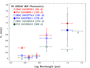
Figure 1.— Observed MIR broadband photometry of SN 2005df at three epochs in Nov. 2005, Feb. 2006, and Aug. 2006. The spectral energy distribution shows little evidence of evolution except for the rapid fading of the IRAC Ch. 1 (3.6 µm) flux between the first two epochs.

Figure 2.— The observed mid-infrared spectrum of SN 2005df. Wavelengths are shown as vacuum coordinates in the observer’s frame, and are plotted on a logarithmic scale so that the observed line width is proportional to the velocity line width throughout the large wavelength span. See text for discussion of line identifications.

Figure 3.— The observed line emission from Co lines in the mid-IR spectrum of SN 2005df on day $\sim 135$, plotted in velocity space relative to the rest frame of the host galaxy.

Figure 4.— The observed line emission from Ni lines in the mid-IR spectrum of SN 2005df on day $\sim 135$, plotted in velocity space relative to the rest frame of the host galaxy.

Figure 5.— The observed line emission from Ar lines in the mid-IR spectrum of SN 2005df on day $\sim 135$, plotted in velocity space relative to the rest frame of the host galaxy. The central vertical dotted line indicates emission at rest relative to the host, while the outer lines indicate the approximate positions of the peaks in the Ar emission at $-4300$ and +6300 km s^-1.

Figure 6.— Observed velocity profiles of three emission features in the mid-IR spectrum of SN 2005df on day $\sim 135$ that could potentially be consistent with [Ni I] emission at high velocity.

Figure 7.— The observed mid-IR spectrum of SN 2003hv compared with that of SN 2005df. Wavelengths are shown as vacuum coordinates in the observer’s frame, and are plotted on a logarithmic scale so that the observed line width is proportional to the velocity line width throughout the large wavelength span. Error bars (based on the output error spectra from the individual order extractions, propagated through the weighted averaging of the orders) are included to help distinguish noise from features in the low S/N spectrum of SN 2003hv. See text for discussion of line identifications.

Figure 8.— The observed line emission from Ar lines in the mid-IR spectrum SN 2003hv on day $\sim 375$, plotted in velocity space relative to the rest frame of the host galaxy. The central vertical dotted line indicates emission at rest relative to the host.

Figure 9.— The observed [Co III] 11.89 µm emission-line profile for SN 2005df on day $\sim 135$, compared to model line emission from a hollow uniform spherical distribution of emission with an inner radius corresponding to a minimum velocity $v_{min}=2500$ km s^-1, and an outer radius corresponding to a maximum velocity $v_{max}=8000$ km s^-1.

Figure 10.— The observed [Co III] 11.89 µm emission-line profile from SN 2005df on day 135, compared with the near-IR emission-line profiles of [Co III] 1.55 µm and [Fe II] 1.64 µm near day 200 (data from Gerardy et al., in prep.)

Figure 11.— The observed [Co III] 11.89 µm emission-line profile from SN 2003hv at 375 d, compared with the 410 d near-IR emission-line profile of [Fe II] 1.64 µm (NIR data from Motohara et al. 2006).

Figure 12.— The observed Ar line profiles in SN 2005df on day $\sim 135$ compared with calculated emission-line profiles for an edge-on equatorial ring model. The emission models for the two profiles differ only in the latitudinal profiles used (see Figure 13), with the [Ar II] emission confined to a narrow region near the equator and the [Ar III] emission coming from a much larger range of latitudes. (See text for further details.)

Figure 13.— The latitudinal angular profile functions used for the models shown in Figure 12.

Figure 14.— The observed Ar line profiles in SN 2005df on day $\sim 135$ compared with calculated emission-line profiles for a pole-on prolate emission geometry with an off-center spherical hole near the middle. (See text for details.)

Figure 15.— Schematic of the model emission used to create the line profiles in Figure 14. Emission is uniformly distributed in prolate ellipsoids with a central spherical hole offset along the line of sight. The figure is to scale with the geometry used for the Ar line profiles in Figure 14.

Figure 16.— Argon distribution from a 2-D model for an off-center delayed-detonation model. The model shown is the same as that described by Fesen et al. (2006), and the color scale is the same as their Figure 7, with red corresponding to the mass-fraction peak, and blue corresponding to zero mass-fraction. The box dimensions correspond to velocities of $\pm 27500$ km s^-1. The model shows a “crescent-shaped” density peak which is perhaps qualitatively similar to one lobe of our prolate Ar emission model (see text for discussion.)

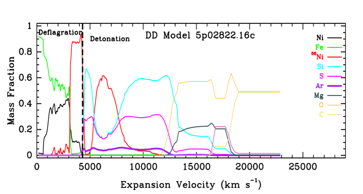
Figure 17.— Abundances for the 5p02822.16 delayed detonation model (H02) plotted versus expansion velocity. For simplicity, many of the less abundant species have not been plotted. The vertical dashed line represents the approximate location of the transition from deflagration to detonation. Material to the left of this line is formed during the deflagration phase, while material to the right is the product of detonation. Note that the small zone of Si/S-rich material near 5000 km s^-1 is an artifact of the imposed spherical symmetry of this model and is not seen in multi-dimensional DD models.

Appendix A Calculation of Nebular Emission-Line Profiles

For nebular supernova emission with negligible sources of continuum opacity and background emission, line profiles can be calculated in the Sobolev approximation by adding up the contributions from differential volume elements in the SN envelope. Adopting the notation of Shu (1991), the contribution to the luminosity emitted toward the line of sight $\mathbf{\hat{k}}$ from material with specific intensity $I_{\nu}$ moving at (large) velocity $\mathbf{u}$ is given by

$$dL_{\nu}(\mathbf{\hat{k}})=4\pi I_{\nu}\left(\frac{\nu_{0}}{c}\right)\mathbf{\hat{k}}\cdot\mathbf{\nabla(\hat{k}}\cdot\mathbf{u})\left(\frac{dV}{d\nu}\right).$$ (A1)

For a homologously expanding envelope with $\mathbf{u}=\frac{R}{t}\mathbf{\hat{r}}$, we have $\mathbf{\hat{k}}\cdot\mathbf{\nabla(\hat{k}}\cdot\mathbf{u})=t^{-1}$. Assuming that the line emission is intrinsically narrow, and placing the line of sight along the $x$ axis, then line emission with a rest-frame frequency $\nu_{0}$ will only contribute to the line profile at observed frequency $\nu$ if $\nu=\nu_{0}\left[1+\frac{v_{x}}{c}\right]=\nu_{0}\left[1+\frac{x}{ct}\right]$. Thus

$$dL_{\nu}(x)=4\pi I_{\nu}\left(\frac{\nu_{0}}{c}\right)t^{-1}\left(\frac{dV}{dx}\right)\left(\frac{dx}{d\nu}\right)=4\pi I_{\nu}\left(\frac{dV}{dx}\right).$$ (A2)

In other words, the luminosity of the line profile at a given observed radial velocity $v_{x}=x/t$ can be calculated by simply integrating the specific intensity of the emitting material in planar volume elements perpendicular to the line of sight. Thus, for a given spatial distribution of $I_{\nu}$, the line profile is, in principle, easy to calculate.

In practice, however, supernovae are easier to describe as close to spherical or axisymmetric, so it is useful to convert this integration over a plane perpendicular to the line of sight, to an integration over spherical coordinates centered on the supernova and inclined at an angle $i$ to the line of sight (such that $i=0$ implies viewing the supernova “pole-on” and $i=90\arcdeg$ corresponds to viewing the supernova equatorially or “edge-on”). In general, the specific intensity distribution can be decomposed into the product of three components,

$$I_{\nu}(r,\psi,\phi)=\rho(r,\psi,\phi)\Psi(\psi,\phi)\Phi(\phi),$$ (A3)

where $r$ and $\phi$ are the standard radial and longitudinal coordinates and $\psi$ is simply the complement of the standard latitudinal coordinate $\theta$. For highly symmetrical distributions, the distribution will decouple further with $\Psi(\psi,\phi)=\Psi(\psi)$ for axisymmetric distributions, and $\rho(r,\psi,\phi)=\rho(r)$ for spherical symmetry. (Note: we chose to use $\psi$ rather than $\theta$ because it slightly simplifies the case of equatorial viewing. This derivation can be relatively easily converted to the standard spherical coordinates by a judicious exchange of sines and cosines and swapping integration limits.)

It is useful to think of the differential volume elements as circular rings of constant $r$ and $\psi$. Each ring will have a radius $R=r\cos\psi$, inclination $i$, and the $x$ coordinate of the center will be at $x_{0}=r\sin\psi\cos i$. For a given radial velocity $v_{r}=x/t$, the ring will only contribute the line profile at (at most) two points $\phi=\pm\phi^{\prime}$ (except for the special case of $i=0$), where $\phi^{\prime}=\cos^{-1}\left[\frac{(x-x_{0})}{r\cos\psi\sin i}\right]$. The differential volume element $dV=r^{2}\cos\psi drd\psi d\phi$, and so combining Equations A2 and A3, we have

$$dL_{\nu}(x) = 4\pi\rho(r,\psi,\phi)\Psi(\psi,\phi)\Phi(\phi)[\delta(\phi-\phi^{\prime})+\delta(\phi+\phi^{\prime})]r^{2}\cos\psi drd\psi\left(\frac{d\phi}{dx}\right)$$

$$= 4\pi\rho(r,\psi,\phi)\Psi(\psi,\phi)\Phi(\phi)[\delta(\phi-\phi^{\prime})+\delta(\phi+\phi^{\prime})]\frac{r^{2}\cos\psi drd\psi}{\sqrt{r^{2}\cos^{2}\psi\sin^{2}i-(x-x_{0})^{2}}}.$$

The total contribution to the line flux at a given radial velocity can thus be found by integrating over those rings that intersect the $x=v/t$ plane. Hence,

$$L_{\nu}(x=v_{r}/t)=\int_{x}^{v_{max}/t}r^{2}\rho(r)\int_{\psi_{min}(r,x)}^{\psi_{max}(r,x)}\Psi(r,\psi)\Phi^{*}(x,\psi,r)\frac{\cos\psi d\psi dr}{\sqrt{r^{2}\cos^{2}\psi\sin^{2}i-(x-x_{0}(r,\psi))^{2}}},$$ (A4)

where

$$\Phi^{*}(x,\psi,r)=\left[\Phi(\phi^{\prime}(x,\psi,r))+\Phi(-\phi^{\prime}(x,\psi,r))\right]$$

for $i\neq 0$ and

$$\Phi^{*}(x,\psi,r)=\int_{0}^{2\pi}\Phi(\phi)d\phi$$

for $i=0$. The latitudinal limits of integration are more complicated, and for a given $r$ depend on the value of $x$ relative to $x_{N}=r\cos i$ and $x_{S}=-r\cos i$, the $x$-coordinates of the $\psi=\pm 90\arcdeg$ poles on a sphere of radius $r$. For a given value of $r$, the latitudinal integration limits are

$$\mbox{For }x_{N}\leq x\leq r\mbox{:}$$

$$\psi_{min}(r,x)=\frac{\pi}{2}-\alpha-i$$

$$\psi_{max}(r,x)=\frac{\pi}{2}+\alpha-i$$

$$\mbox{For }0\leq x<x_{N}\mbox{:}$$

$$\psi_{min}(r,x)=\frac{\pi}{2}-\alpha-i$$

$$\psi_{max}(r,x)=\frac{\pi}{2}-\alpha+i$$

$$\mbox{For }x_{S}\leq x<0\mbox{:}$$

$$\psi_{min}(r,x)=-\frac{\pi}{2}+\alpha-i$$

$$\psi_{max}(r,x)=-\frac{\pi}{2}+\alpha+i$$

$$\mbox{For }-r\leq x<x_{S}\mbox{:}$$

$$\psi_{min}(r,x)=-\frac{\pi}{2}-\alpha+i$$

$$\psi_{max}(r,x)=-\frac{\pi}{2}+\alpha+i$$

where $\alpha=\cos^{-1}(\frac{|x|}{r})$.

For the line profiles presented in this work, the radial, latitudinal, and longitudinal specific intensity distribution functions (Eqn A3) were coded in Python and Equation A4 numerically integrated using the quadpack algorithms in the SciPy software package.

Figure 18.— Calculated emission-line profiles for three simple emission geometries: a uniform sphere (left), a uniform thin spherical shell (center), and a uniform thin circular ring (right).

The resulting line profiles from simple emission geometries are shown in Figure 18. A homogeneous sphere of emission produces the well-known parabolic line-profile shape, while a thin, uniformly emitting spherical shell produces a “top-hat” line profile, and a thin, uniformly emitting ring produces a forked profile [$F\propto(1-(v/v_{max})^{2})^{-1/2}$]. Since the volume integration in Equation A4 is “additive,” it is often useful to think of the emission from more complicated geometries as linear combinations of simpler emission geometries. Thus a thick sphere of emission with a central hole can be built up either by adding “top-hat” line profiles from progressively larger shells, or by subtracting the line profile from a small homogeneous sphere from that of a larger homogeneous sphere. In both cases one ends up with a line profile that is flat (shell-like) in the core, and parabolic (sphere-like) in the wings.

References

- Aitken et al. (1988) Aitken, D. K., Smith, C. H., James, S. D., Roche, P. F., Hyland, A. R., & McGregor, P. J. 1988, MNRAS, 235, 19
- Axelrod (1980) Axelrod, T. S., 1980, PhD Thesis, UCRL-52994, Univ. California, Santa Cruz
- Badenes et al. (2006) Badenes, C., Borkowski, K. J., Hughes, J. P., Hwang, U., & Bravo, E. 2006, ApJ, 645, 1373
- Bautista (2001) Bautista, M. A. 2001, A&A, 365, 268
- Benetti et al. (2004) Benetti, S., et al. 2004, MNRAS, 348, 261
- Beutler & Li (2003) Beutler, B., & Li, W. 2003, IAU Circ. 8197
- Bowers et al. (1997) Bowers, E. J. C., Meikle, W. P. S., Geballe, T. R., Walton, N. A., Pinto, P. A., Dhillon, V. S., Howell. S. B., & Harrop-Allin, M. K. 1997, MNRAS, 290, 663
- Branch (1998) Branch, D. 1998, ARA&A, 36, 17
- Catchpole et al. (1988) Catchpole, R. M., et al. 1988, MNRAS, 231, 75
- Colgate & McKee (1969) Colgate, S. A., & McKee, C. 1969, ApJ, 157, 623
- Kozma et al. (2005) Kozma, C., Fransson, C., Hillebrandt, W., Travaglio, C., Sollerman, J., Reinecke, M., Röpke, F. K., & Spyromilio, J. 2005, A&A, 437, 983
- Dressler et al. (2003) Dressler, A., Phillips, M., Morrell, N., & Hamuy, M. 2003, IAU Circ. 8198
- Eastman et al. (1996) Eastman, R. G., Schmidt, B. P., & Kirshner, R. 1996, ApJ, 466, 911
- Evans (2005) Evans, R. 2005, IAU Circ. 8580
- Fazio et al. (2004) Fazio, G. et al. 2004, ApJS, 154, 10
- Fesen et al. (2006) Fesen, R. A., Höflich, P., Hamilton, A. J. S., Hammel, M. C., Gerardy, C. L., Khokhlov, A. M., Wheeler, J. C. 2006, ApJ, submitted
- Filippenko (1997) Filippenko, A. V. 1997, ARA&A, 35, 309
- Galavís, Mendoza, & Zeippen (1995) Galavís, M. E., Mendoza, C., & Zeippen, C. J. 1995, A&A, 111, 347
- Gamezo, Khokhlov, & Oran (2004) Gamezo, V. N., Khokhlov, A. M., & Oran, E. S. 2004, Phys. Rev. Lett., 92, 211102
- Gamezo, Khokhlov, & Oran (2005) Gamezo, V. N., Khokhlov, A. M., & Oran, E. S. 2005, ApJ, 623, 337
- Gibson et al. (2000) Gibson, B. K., et al. 2000, ApJ, 529, 723
- Gilmore (2005) Gilmore, A. 2005, IAU Circ. 8580
- Graham, Wright, & Longmore (1987) Graham, J. R., Wright, G. S., & Longmore, A. J. 1987, ApJ, 313, 847
- Halenka (1989) Halenka, J. 1989, A&A, 81, 303
- Halenka et al. (2001) Halenka, J., Madej, J., Langer, K., & Mamok, A. 2001, Acta Astron., 51, 347
- Hamuy (2002) Hamuy, M. 2002, ApJ, 582, 905
- Höflich et al. (1995) Höflich, P., Khokhlov, A. M., & Wheeler, J. C. 1995, ApJ, 444, 831
- Höflich et al. (2002) Höflich, P., Gerardy, C. L., Fesen, R. A., & Sakai, S. 2002, ApJ, 568, 791 (H02)
- Höflich et al. (2003) Höflich, P., Gerardy, C. L., Linder, E., & Marion, G. H. 2003, in Stellar Candles for the Extragalactic Distance Scale, ed. D. Alloin & W. Gieren (Berlin: Springer), 203
- Höflich et al. (2004) Höflich, P., Gerardy, C. L., Nomoto, K., Motohara, K., Fesen, R. A., Maeda, K., Ohkubo, T., Tominaga, N. 2004, ApJ, 617, 1258
- Houck et al. (2004) Houck, J., et al. 2004, ApJS, 154, 18
- Howell et al. (2001) Howell, D. A., Höflich, P., Wang, L., & Wheeler, J. C. 2001, ApJ, 556, 302
- Irwin (1981) Irwin, A. W. 1981, ApJS, 45, 621
- Kasen et al. (2004) Kasen, D., Nugent, P., Thomas, R. C., & Wang, L. 2004, ApJ, 610, 876
- Kotak et al. (2005) Kotak, R., Meikle, P., van Dyk, S. D., Höflich, P. A., & Matilla, S. 2005, ApJ, 628, 123
- Kotak et al. (2006) Kotak, R., et al. 2006, ApJ submitted.
- Khokhlov (1991) Khokhlov, A. M. 1991, A&A, 245, 114
- Leibundgut (2001) Leibundgut, B. 2001, ARA&A, 39, 67
- Liu, Jeffery, & Schultz (1997) Liu, W., Jeffery, D. J., & Schultz, D. R. 1997, ApJ, 483, 107
- Marietta et al. (2000) Marietta, E., Burrows, A., & Fryxell, B. 2000, ApJS, 128, 615
- Marion et al. (2003) Marion, G. H., Höflich, P., Vacca, W. D., & Wheeler, J. C. 2003, ApJ, 591, 316
- Motohara et al. (2006) Motohara, K., Maeda, K., Gerardy, C. L., Nomoto, K., Tanaka, M., Tominaga, N., Ohkubo, T., Mazzali, P. A., Fesen, R. A., Höflich, P., Wheeler, J. C. 2006, ApJ, 652, 101
- Meléndez & Bautista (2005) Meléndez, M., & Bautista, M. A. 2005, A&A, 436, 1123
- Nomoto (1982) Nomoto, K. 1982, ApJ, 257, 780
- Nomoto, Thielemann, & Yokoi (1984) Nomoto, K., Thielemann, F.-K. & Yokoi, K. 1984, ApJ, 286, 644
- Nomoto et al. (2003) Nomoto, K., Uenishi, T., Kobayashi, C., Umeda, H., Ohkubo, T., Hachisu, I., & Kato, M. 2003, in From Twilight to Highlight: The Physics of Supernovae, ed. W. Hillebrandt, & B. Leibundgut (Berlin: Springer), 115
- Nussbaumer & Storey (1988) Nussbaumer, H., & Storey, P. J. 1988, A&A, 200, 25
- Pelan & Berrington (1995) Pelan, J., & Berrington, K. A. 1995, A&A, 110, 209
- Plewa, Calder, & Lamb (2004) Plewa, T., Calder, A. C., & Lamb, D. Q. 2004, ApJ, 612, 37
- Quinet & Le Dourneuf (1996) Quinet, P., & Le Dourneuf, M. 1996, A&A, 119, 99
- Quinet (1998) Quinet, P. 1988, A&A, 129, 147
- Riess et al. (1999) Riess, A. G., et al. 1999, AJ, 118, 2675
- Roche, Aitken, & Smith (1991) Roche, P. F., Aitken, D. K., & Smith, C. H. 1991, MNRAS, 252, 39
- Röpke (2005) Röpke, F. K. 2005, A&A, 432, 969
- Röpke et al. (2006) Röpke, F. K., Gieseler, M., Reinecke, M., Travaglio, C., & Hillebrandt, W. 2006, A&A, 453, 203
- Ruiz-Lapuente et al. (1995) Ruiz-Lapuente, P., Kirshner, R. P., Phillips, M. M., Challis, P. M., Schmidt, B. P., Filippenko, A. V., & Wheeler, J. C. 1995, ApJ, 439, 60
- Salvo & Schmidt (2005) Salvo, M., & Schmidt, B. 2005, IAU Circ. 8581
- Schmidt et al. (1994) Schmidt, B. P., Kirshner, R. P., Eastman, R. G., Maza, J. & Avilés, R. 1994, ApJ, 432, 42
- Schlegel et al. (1998) Schlegel, D. J., Finkbeiner, D. P., & Davis, M. 1998, ApJ, 500, 525
- Shu (1991) Shu, F., The Physics of Astrophyics, Volumne 1: Radiation (Mill Valley: University Science Books)
- Sollerman et al. (2004) Sollerman, J., Lindahl, J., Kozma, C., Challis, P., Filippenko, A. V., Fransson, C., Garnavich, P. M., Leibundgut, B., Li, W., Lundqvist, P., Milne, P., Spyrimilio, J., & Kirshner, R. P. 2004, A&A, 428, 555
- Stritzinger et al. (2006) Stritzinger, M., Mazzali, P. A., Sollerman, J., & Benetti, S. 2006, A&A, 460, 793
- Tonry et al. (2000) Tonry, J. L., Blakeslee, J. P., Ajhar, E. A., & Dressler, A. 2000, ApJ, 530, 625
- Werner et al. (2004) Werner, M., et al. 2004, ApJS 154, 1
- Wooden (1989) Wooden, D. 1989, PhD Thesis, University of California, Santa Cruz
- Yamaoka et al. (1992) Yamaoka, H., Nomoto, K., Shigeyama, T., Thielemann, F.-K. 1992, ApJ, 393, 55