On the intermittent character of
interplanetary magnetic field fluctuations

Abstract

Interplanetary magnetic field magnitude fluctuations are notoriously more intermittent than velocity fluctuations in both fast and slow wind. This behaviour has been interpreted in terms of the anomalous scaling observed in passive scalars in fully developed hydrodynamic turbulence. In this paper, the strong intermittent nature of the interplanetary magnetic field is briefly discussed comparing results performed during different phases of the solar cycle. The scaling properties of the interplanetary magnetic field magnitude show solar cycle variation that can be distinguished in the scaling exponents revealed by structure functions. The scaling exponents observed around solar maximum coincide, within the errors, to those measured for passive scalars in hydrodynamic turbulence. However, it is also found that the values are not universal in the sense that the solar cycle variation may be reflected in dependence on the structure of the velocity field.

I Introduction

The interplanetary medium is pervaded by fluctuations providing information on plasma turbulence on a large range of scales, from fractions of second up to the solar rotation period Tu and Marsch (1995). Some characteristic features of these fluctuations include Bruno and Carbone (2005) strong anisotropy shown by velocity and magnetic field fluctuations, the different radial evolution of the minimum variance direction of the magnetic field (hereafter IMF) and velocity, the lack of equipartition between magnetic and kinetic fluctuations as well as scaling and non- Gaussian Probability Density Functions (PDF) of flux densities Hnat et al. (2003). All those factors contribute to the view that statistical properties of the solar wind should be far from that of Kolmogorov Kolmogorov (1941) for fluid turbulence which assumes isotropic, homogeneous and incompressible flow.

However, as shown since the first in situ observations Coleman (1968), fluctuations measured in the solar wind plasma parameters share many statistical features with fluctuations observed in hydrodynamic turbulence Tu and Marsch (1995); Bruno and Carbone (2005). For example, the problem of intermittency, namely the departure from statistical self-similarity, has been investigated on the basis of standard techniques and modelling Bruno and Carbone (2005). The “strength” of intermittency, related to the ability of the turbulent cascade to develop singularities at small scales, can be quantified by measuring the scaling exponents $\zeta_{p}$. These are defined through the structure functions $S_{p}(\tau)=\langle(\delta v_{\tau})^{p}\rangle\sim\tau^{\zeta_{p}}$, where $\delta v_{\tau}(t)=v(t+\tau)-v(t)$ are the velocity fluctuations over a given scale $\tau$ Frisch (1995); Burlaga (1991); Bruno and Carbone (2005). Similarly, we can define structure functions, and exponents, for fluctuations in temperature, magnetic field magnitude or density in order to investigate their scaling properties.

The scaling exponents for velocity and magnetic field Hnat et al. (2005a); Burlaga (1991); Carbone et al. (1995) are nonlinear in $p$, departing from the Kolmogorov non-intermittent scaling $\zeta_{p}=p/3$ Kolmogorov (1941); Frisch (1995). The scale dependent character of the field fluctuations can also be observed from the shape of the PDFs of the fields Marsch and Liu (1993); Sorriso–Valvo et al. (1999). In this case the PDFs of fluctuations standardized with their relative standard deviation increasingly depart from a Gaussian distribution with decreasing temporal scale $\tau$. Recent studies have shown that the slow wind is more intermittent than the fast wind and, as largely reported in literature, the solar wind magnetic field is more intermittent than the velocity field Marsch and Liu (1993); Carbone et al. (1995); Sorriso–Valvo et al. (1999); Carbone et al. (2004); Bruno and Carbone (2005). The difference between velocity and magnetic field intermittency has also been observed in two-dimensional incompressive magnetohydrodynamics (MHD) numerical simulations Politano et al. (1998); Sorriso-Valvo et al. (2001a, b); Merrifield et al. (2007c), and seems to be a robust feature of MHD turbulence. Such behaviour is similar to the transport of passive fields in fully developed hydrodynamic turbulence where the advected field (usually temperature) is more intermittent than the advecting velocity field Falkovich et al. (2001). This suggests a similarity between statistical features of the interplanetary magnetic field strength and hydrodynamic passive scalars Sorriso–Valvo et al. (1999); Carbone et al. (2004); Bruno and Carbone (2005). The question then arises as to whether these similarities are a consequence of shared dynamical behaviour. Indeed, the magnetic field plays a relevant role in both velocity shear instability and parametric instability during the development of the turbulence spectrum observed in the solar wind Malara et al. (2000); Bavassano et al. (2000).

Figure 1 shows the behaviour of scaling exponents $\zeta_{p}$ versus order $p$, computed through the Extended Self-Similarity technique Benzi et al. (1993) and normalized to the third order scaling exponent $\zeta_{3}$ for both solar wind velocity and magnetic field, as compared with results from passive scalar transported by incompressible hydrodynamic turbulence. The interplanetary data were obtained during a slow wind interval observed at the Helios 2 satellite at 0.9 AU while the fluid data derive from the experiment Benzi et al. (1999). We can see from the plot that the exponents for the magnitude of velocity for both fluid and solar wind approximately coincide, as do those of the solar wind magnetic field magnitude and the fluid passive scalar. The question then is whether or not such behaviour can be ascribed to the passive nature of the interplanetary magnetic field and as such is universal.

Passive scalar dynamics for the interplanetary magnetic field (IMF) magnitude would have far reaching consequences for the theoretical description and the modelling of solar wind turbulence. For example, if the magnetic field could be treated as a passive vector the observed Kolmogorov-like spectra of the solar wind Tu and Marsch (1995) could be explained using hydrodynamic turbulence. In this paper, we test whether this ’passive scalar’ signature in the IMF is robust by comparing scaling properties of the IMF magnitude at solar minimum and maximum derived from ACE and WIND spacecraft data sets. Previous studies of the energy input that the solar wind provides to the magnetosphere have shown that a measure of the solar wind Poynting flux shows scaling with exponents that vary with the solar cycle Hnat et al. (2005b).

II Data Analysis

We will now test whether or not the passive scalar characteristics of interplanetary magnetic field intensity fluctuations are found consistently during different solar cycle phases. If the IMF magnitude is intrinsically a passive scalar, its scaling should be robust against the particular data sample that we choose, provided that the fluctuations are in a state of fully developed turbulence. We will first perform an analysis of the data sets corresponding to extended intervals around solar minimum and maximum. We utilise two data sets, from the WIND and ACE spacecraft. The $92$ second average WIND spacecraft data spanning a single year $1996$ will provide our solar minimum sample, whilst the ACE spacecraft $64$ second average data from the year $2000$ will provide our solar maximum sample.

Figure 2 shows the structure functions of magnetic field magnitude for solar minimum and maximum respectively (offset vertically for clarity). The common scaling region from which these structure functions are obtained are shown by the solid lines on the Figure 2, these represent the best regression fits for temporal scales $\tau$ between $\sim 10$ minutes and $\sim 10$ hours. These scaling regions can be significantly extended, for both data sets, by means of Extended Self-Similarity (ESS). The ESS method seeks scaling $S_{m}(\tau)\!\propto\!S_{p}^{\eta(m)}(\tau)$ which should emerge on a plot of $S_{m}$ versus $S_{p}$. We plot $S_{m}$ versus $S_{4}$ on logarithmic axes for fluctuations in $B$, for solar minimum and maximum in Figure 3 (a,b) respectively. We use this extended scaling range to obtain an improved estimate of the exponents $\tilde{\zeta}(m)\!=\!\zeta(4)\eta(m)$, where $\zeta(4)=0.78\pm 0.03$ for solar minimum and $\zeta(4)=1.01\pm 0.03$ for solar maximum.

Figure 4 combines scaling exponents $\zeta(4)\eta(m)$ obtained from ESS for the magnetic field intensity fluctuations during solar minimum and maximum. For comparison, we have also plotted scaling exponents obtained from the data set used in Ref. Bershadskii and Sreenivasan (2004). The result clearly demonstrates that the magnetic field magnitude fluctuations do not exhibit a single and universal scaling that coincides with that found in the fluctuations of passive scalars in hydrodynamic turbulence. It is also clear, however, that there is a very good agreement between scaling exponents found in Ref. Bershadskii and Sreenivasan (2004) and these derived here from the data set corresponding to solar maximum. Recently, it has been suggested that the large and statistically under-represented events can obscure the underlying statistical properties of turbulent data sets Chapman et al. (2005). A conditioning method has been proposed to filter out a limited number of data points and obtain robust scaling properties of the remaining data. We have verified that such conditioning does not change the qualitative difference between solar minimum and maximum, nor the individual scaling exponents which vary within the error bars. This is qualitatively very different from for example the behaviour of the density fluctuations which exhibit substantial differences between non-filtered and filtered data sets Hnat et al. (2005a).

To gain a better appreciation of the different scaling regimes of the IMF magnitude under changing velocity field we will now focus on different short time intervals with pronounced, well defined structures. Examining these short intervals has the advantage over the study of extended intervals in that we can identify the morphology of individual sequences of data with particular scaling behaviour. However, the disadvantage is that these shorter intervals necessarily reduces the number of data points available, thus we cannot repeat the full structure function analysis above.

The top panel of Figure 5 shows the wind speed profile during $30$ days of data recorded by WIND when the spacecraft passed through two corotating high velocity streams beginning on day $30$ and day $43$, respectively. The bottom panel highlights the different plasma regimes explored by the magnetic field intensity. This parameter is highly compressed at the stream interface, especially where the interface is more developed, and much less within the trailing edge of the stream. Moreover, the low velocity wind (between days 36 and 42) shows the typical compressive region of the interplanetary current sheet (see references cited in Bruno and Carbone (2005)). The four vertical dashed lines and the three different symbols identify three different regions where we quantify the intermittent character of the fluctuations by looking at the flatness factor of the different probability distribution functions at different scales (see Table 1 for data description). Following Frisch (1995), a random function is intermittent at small scales if the flatness of its fluctuations grows without bound at smaller and smaller scales. Figure 6 shows that the three different regions show different values of the flatness, and suggest that the most compressive region, which display the highest $rms$ values of the IMF (see Table 1), is also the most intermittent region.

The information obtained from the statistics of extended intervals, where the solar wind morphology is not specified, and from “hand selected” shorter intervals of known morphology, is complementary but not necessarily coincident. Extended studies will tend to be dominated by the scaling properties of the bulk of the data (see, for example Hnat et al. (2004)). In this context the presence of large scale coherent structures will tend to destroy the scaling, this effect can be removed by conditioning the data (removing isolated outliers as above). To maintain good statistics however, the extended interval should clearly not be dominated by large scale structures such as stream-stream interfaces, Coronal Mass Ejections and interplanetary shocks which are distinct from the evolving turbulence. Short intervals, selected by morphology, explicitly remove these large scale coherent structures. The dynamical interactions experienced by the solar wind during its expansion Tu and Marsch (1995) would be expected to deviate from the ideal condition of incompressibility particularly in the vicinity of these structures.

Table 1: The periods of WIND measurements used in this work: average and root mean square velocity and IMF, and the size of each dataset.

days of 1996	$\langle V\rangle(Km/s)$	$V_{rms}(nT)$	$\langle B\rangle(Km/s))$	$B_{rms}(nT)$	data points
$26$—$31$	$496$	$160$	$7.22$	$4.22$	$1495$
$31$—$36$	$622$	$34$	$5.31$	$0.89$	$1772$
$36$—$41$	$407$	$32$	$7.07$	$2.83$	$1798$

III Comparison with other studies

It is worthwhile to discuss these results in the context of the Ref. Bershadskii and Sreenivasan (2004) where the authors performed similar analysis on a data sample recorded by ACE during $1998$, that is close to solar minimum. The values of scaling exponents, however, were close to these obtained here for solar maximum and it was concluded, showed passive scalar behaviour. How can we explain this contradiction? The year $1998$, although not coincident with the solar maximum of activity cycle $23$, was already characterized by an enhanced coronal activity if compared to the preceding solar minimum, about two years before Gopalswamy et al. (2004). Contrary to what has been stated in Ref. Bershadskii and Sreenivasan (2004), the sun was certainly not quiet at all during this period, and as reported by Ref. Gopalswamy et al. (2004), the CME daily rate was about $4.5$ compared to a rate of approximately $0.5$ around the preceding solar activity minimum which can be considered a truly quiet period. However, different phases of the solar activity cycle are also distinguishable because of a completely different organization of the large scale IMF (see the review Bruno and Carbone (2005) and references therein).

It was also proposed in Ref. Bershadskii and Sreenivasan (2004) that the necessary conditions for the magnetic field magnitude evolution equation to be in the form of advection-diffusion equation. The generic evolution equation takes form:

$$\partial_{t}B=-({\bf u}\cdot\nabla)B+\eta\nabla^{2}B+\lambda B\ ,$$ (1)

where $\bm{u}$ is an incompressible velocity field, $\eta$ is the magnetic diffusivity and $\lambda$ is a pseudo dissipation coefficient given by

$$\lambda=n_{\alpha}n_{\beta}\,\partial_{\alpha}v_{\beta}-\eta\,\partial_{\alpha}n_{\beta}\,\partial_{\alpha}n_{\beta}\ ,$$ (2)

while the vector $\bm{n}=\bm{B}/B$ is the unit vector in the magnetic field direction. The similar scaling observed for the magnetic field magnitude and the passive scalar advected by hydrodynamic turbulence suggests conditions in which the $\lambda$ stretching term could vanish, in which case the evolution of the magnetic field magnitude would reduce to that of a passive scalar Bershadskii and Sreenivasan (2004). However in Bershadskii and Sreenivasan (2004) only conditions in which the first term of (2) would vanish were considered, with the assumption that the second term must be small since the magnetic diffusivity  $\eta$ must be small. While the precise value of $\eta$ in the solar wind is unknown, it must indeed be small since the magnetic Reynolds number ${\rm Re}_{\rm m}=UL/\eta$ is observed to be large Matthaeus et al. (2005); however it does not necessarily follow that the second term of (2) is small. In turbulence at large Reynolds number the gradients of the field or the gradients of the field directions (because the field value themselves are bounded by a few times $B_{\rm rms}$) can become very large, in order to maintain a finite limit of the dissipation when the diffusivity $\eta$ goes to zero. Such “extreme” gradients have been observed (Bruno et al. (2001)), in which the magnetic field changes direction in an abrupt fashion, while keeping its magnitude unchanged. In these cases, it is precisely this second term which is responsible for preserving $B$, because it then acts as a damping term which cannot be neglected. This second term in addition has a well defined (negative) sign and thus cannot vanish by averaging.

In order for (1) to be similar to a passive scalar evolution equation, the first term of (2) should also vanish and some conditions in which this could be realised are given in Bershadskii and Sreenivasan (2004). However these conditions are not realised most of the time, and not in the fast solar wind Bruno and Carbone (2005). The conditions are essentially loss of correlation between the magnetic field direction and of the velocity gradient, however this will not be the case in Alfvénic turbulence in the fast wind, where the velocity and magnetic fields follow each other closely, anticorrelated (for outward Alfvén waves) or correlated (for inward waves) fashion Bruno and Carbone (2005). In these cases, the magnitudes of $\bm{B}$ and $\bm{u}$ also follow each other closely, and it is clear that $B$ cannot be considered as a passive scalar. The first term of (2) then also ensures the reaction of the magnetic field on the velocity and the equipartition between magnetic and kinetic energy. Recent studies also indicate that the assumption of incompressibility of the plasma is not consistent with passive scalar behaviour in the solar wind Hnat et al. (2005a).

IV Conclusions

The aim of this study was to gain a better understanding of the scaling properties of the IMF magnitude and its dependence on the changing solar wind velocity field. Our results show a remarkable similarity between the scaling exponents of passive scalars in hydrodynamic turbulence and the IMF magnitude during solar maximum. At $\approx 1$ AU, slow streams that originate from the near-equatorial region of the Sun, dominate the solar wind at solar maximum. This result is in agreement with our Figure $1$, where scaling properties of slow solar wind streams were presented. We draw the readers attention to the fact that the scaling of the velocity fields for the hydrodynamic flow and the solar wind also exhibit nearly identical scaling in that case. Statistical properties of the passive fluctuations are known to depend strongly on the characteristics of the advecting velocity field Frisch et al. (1999). In that respect it is not surprising that the scaling properties of the IMF magnitude change dramatically with the solar cycle.

Further work is needed to establish how universal these scaling properties of the IMF magnitude really are. This could be done by applying conditional statistics, that is deriving the scaling properties of $B$ from the data sets with similar velocity profiles. If scaling exponents derived from these intervals are robust we could then accept the scaling as universal. This is, however, a rather daunting task, as illustrated by Figure $5$. The analysis requires long data sets in order to obtain the scaling exponents with sufficient precision, however the velocity profile of the solar wind is very dynamic, leaving us with relatively short time intervals.

We now arrive to the most intriguing question: Is the magnetic field magnitude passively advected in the solar wind? It is clear that one can draw only partial conclusions from our results. We have shown that there is some evidence, based on scaling properties of the IMF magnitude, that the passive scalar model for $|B|$ could, indeed, be valid for the slow solar wind. The universality of the scaling is, however, still to be addressed. This is even more so for the fast solar wind where the departure from the known hydrodynamic scaling is very pronounced.

We also point out the apparent difficulty in relating the known features of the slow and fast streams of the solar wind to the assumptions of Ref Bershadskii and Sreenivasan (2004) which led to an evolution equation for $|B|$ written as an advection-diffusion one. The assumptions used for this were: (i) incompressibility of the flow ($\nabla\cdot\bm{u}=0$), and (ii) the isotropy of the average direction of the magnetic field. While the incompressibility assumption may be justified for the fast wind streams (solar minimum) it is much harder to extend its applicability to the slow wind (solar maximum). The average isotropy of the magnetic field direction is even harder to realise in solar wind turbulence, which is inherently anisotropic. As a corollary, the applicability of “ideal” phenomenologies such as Irosnikov-Kraichnan is an open question, since the solar wind is anisotropic (background magnetic field) and asymmetric (Alfvén wave fluxes tend to be away from the sun) and compressible Hnat et al. (2005a).

It might thus be that the coincidence of the magnetic field magnitude scaling exponents and those of passive scalars is fortuitous, especially given the fact that the advecting velocity fields are different. Indeed, one arises from strongly coupled MHD turbulence, and the other from incompressible fluid turbulence, and it has been ascertained that the intermittency properties of passively advected scalars do depend on the velocity field Celani et al. (2001); Falkovich et al. (2001). The similarity of scaling does therefore not imply a similarity of dynamics, as already noted by Hnat et al. (2005a); Sorriso-Valvo et al. (2006). We finally offer an alternative dynamical model that can explain the increased intermittency of the $|B|$ fluctuations.

It has been shown that the stronger intermittency of the passive scalar reflects the presence of sharp gradients of the field within its stochastic fluctuations  Sreenivasan (1991); Warhaft (2000); Celani et al. (2001). This peculiar behaviour could be the signature of the advected field being trapped in coherent structures, generated by the turbulent cascade in the velocity field. Such large gradients are characteristic of the slow solar wind (solar maximum) which is populated with transition zones, that is shearing zones and shocks. The effect of adding the strong gradients between the zones is that of increased intermittency which, in turn, makes the behaviour more similar to that of a passive scalar advected by ordinary turbulence. If this is the dominant dynamics in an extended interval of data, then it will dominate the scaling exponents.

FIG. 1 CAPTION - The normalized scaling exponents $\zeta_{p}$ as a function of the moment order $p$ are reported, along with the linear expected value $p/3$ (full line). Data refers to the bulk velocity (black circles) and the magnitude of the magnetic field (white circles), as measured by the Helios 2 satellite in the inner heliosphere at $0.9$ Astronomical Units during slow wind streams. Scaling exponents have been obtained through the Extended Self-Similarity technique. Reported for comparison are the normalized scaling exponents for longitudinal velocity field (stars) and the temperature field (passive scalar) in usual fluid flow.

FIG. 2 CAPTION - (Color online) Structure functions of interplanetary magnetic field derived from: (a) WIND data for the solar minimum of 1996 and (b) ACE spacecraft data for the solar maximum of 2000. Solid lines represent the best linear fit to the points between temporal scales $\sim 10$ minutes and $\sim 10$ hours.

FIG. 3 CAPTION - (Color online) ESS derived from (a) WIND data for the solar minimum of 1996 and (b) ACE spacecraft data for the solar maximum of 2000. Solid lines represent the best linear fit to the points between temporal scales $\sim 1$ minute and $\sim 10$ hours.

FIG. 4 CAPTION - (Color online) Scaling exponents from ESS of the magnetic field magnitude fluctuations for solar minimum (empty circles), solar maximum (filled circles) and the ACE interval for $1998$ (triangles).

FIG. 5 CAPTION - Top panel: wind speed profile during 30 days of data recorded by WIND. Bottom panel: magnetic field intensity profile. The four vertical dashed lines and the three different symbols identify three different regions where we evaluated the intermittent character of the fluctuations.

FIG. 6 CAPTION - Flatness factor versus time scale relative to the three different time intervals shown in the previous Figure.

Figure 1:

.475 .475

Figure 2:

.475 .475

Figure 3:

.75

Figure 4:

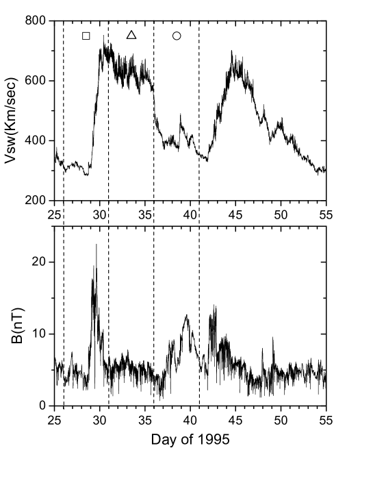
Figure 5:

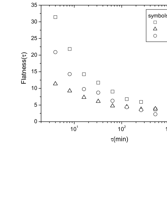
Figure 6: