WHAT DRIVES OUR ACCELERATING UNIVERSE?

Abstract

The homogeneous expansion history $H(z)$ of our universe measures only kinematic variables, but cannot fix the underlying dynamics driving the recent acceleration: cosmographic measurements of the homogeneous universe, are consistent with either a static finely-tuned cosmological constant or a dynamic ‘dark energy’ mechanism, which itself may be material Dark Energy or modified gravity (Dark Gravity). Resolving the dynamics of either kind of ‘dark energy’, will require complementing the homogeneous expansion observations with observations of the growth of cosmological fluctuations. Because the ’dark energy’ evolution is, at most, quasi-static, any dynamical effects on the fluctuation growth function $g(z)$ will be minimal. They will be best studied in the weak lensing convergence of light from galaxies at $0<z<5$, from neutral hydrogen at $6<z<20$, and ultimately from the CMB last scattering surface at z=1089. Galaxy clustering also measures $g(z)$, but requires large corrections for baryonic composition and foreground noise to reduce their large systematic errors.

Projected observations may potentially distinguish static from dynamic ‘dark energy’, but distinguishing dynamic Dark Energy from Dark Gravity will require a weak lensing shear survey more ambitious than any now projected. Low-curvature modifications of Einstein gravity are also, in principle, observable in the solar system or in isolated galaxy clusters.

The Cosmological Constant Problem, that quantum material vacuum fluctuations apparently do not gravitate, suggests identifying gravitational ’vacuum energy’ with classical intrinsic spacetime curvature, rather than with any quantum material property. This spacetime curvature of empty space appears cosmologically and about isolated sources and can only be fine-tuned, at present. The Cosmological Coincidence Problem, that we live when the ordinary matter density approximates the ’gravitational vacuum energy’, on the other hand, is a material problem, calling for an understanding of the observers’ role in cosmology.

I INTRODUCTION: COSMOLOGICAL SYMMETRY VS. DYNAMICS

The most surprising recent cosmological discovery is that the expansion of our universe began accelerating recently, about redshift $z\sim 0.5$. This paper will stress the distinction between the description of the expanding universe (cosmography or kinematics) and the mechanism driving this accelerating expansion (’dark energy’ or dynamics). Because the homogeneous expansion $H(z)$ measures only kinematic variables, it cannot fix the underlying dynamics: cosmographic measurements of our late accelerating universe, are consistent with either a static cosmological constant or a dynamic ‘dark energy’, which itself may be a newly-revealed negative pressure material within General Relativity (GR) or modified gravity (Dark Gravity) Gu and Hwang (2001); Sahni and Starobinsky (2006). Indeed, the expansion history probes only one of the gravitational field equations, the Friedmann equation in General Relativity or a modified Friedmann equation in modified gravity.

Starting from the observed global homogeneity, isotropy and spatial flatness of the universe (flat Robertson-Walker cosmology, RW), Section II will emphasize the difference between this RW symmetry and the dynamics driving the cosmological acceleration. Quotation marks are used to stress that ‘dark energy’ and its ’equation of state’ merely summarize the expansion history. Because we are interested in distinguishing Dark Gravity from Dark Energy, we are careful not to identify RW cosmology with GR, as do many texts and authors.

We want to know whether ’dark energy’ is static or dynamic and whether a newly-revealed material constituent within General Relativity (Dark Energy), or a low-curvature modification of General Relativity (Dark Gravity). We will revert to Einstein’s original definition of his cosmological constant $4\Lambda$ as a classical intrinsic (Ricci) spacetime curvature $R_{dS}$ of empty spacetime, the ground state of gravitational theory. Thus, we will interpret the cosmological constant geometrically. By disconnecting the cosmological constant from material sources, this identification of Dark Gravity with geometry avoids addressing the Cosmological Constant Problem, why quantum vacuum energies apparently do not gravitate in four dimensions. This Cosmological Constant Problem is clearly a far infra-red gravity problem, not directly connected with four-dimensional quantum gravity. Brane cosmologies invoke extra space dimensions to bridge the huge energy gap between ordinary gravity and other fields, they solve the Cosmological Constant Problem only by fine-tuning the very small scale of these extra dimensions.

Although ’dark energy’ may not be energy at all, but only spacetime curvature, we adhere to common parlance by denoting as ’gravitational vacuum energy’ $\rho_{vac}:=M_{P}^{2}\Lambda=M_{P}^{2}R_{dS}/4$, the vacuum spacetime curvature $R_{dS}$ or the cosmological constant $\Lambda$, up to dimensional factors in the Planck mass $M_{P}$. This intrinsic spacetime curvature or vacuum energy has generic dynamical consequences which we will discuss in Section III: It distinguishes high- from low-curvature modifications of Einstein gravity; It modifies the gravitational field surrounding an isolated source, already at a Vainstain radius $r_{*}$, much smaller than the de Sitter radius $H_{dS}^{-1}$. These examples will help clarify the physical significance of ’dark energy’.

Section IV will expose the limitations of observations of the homogeneous expansion: the expansion history observed in the supernova (SN), baryon acoustic oscillation (BAO)) and CMB is simply consistent with the Classical Cosmological Constant Model $\Lambda$CDM), with a small static cosmological constant $\Lambda$, but also allows a ‘dark energy’ that is now nearly static. Table III, derived from Davis et al. (2007); Wood-Vasey et al. (2007) with some additions in the right column, shows that no present data requires dynamic ’dark energy’. If dynamic, the common ’equation of state’ parametrization (11) assumes that it remains quasi-static at high redshifts $z>2$, an assumption that will be tested only after much more gravitational weak lensing (WL) data is observed.

The ‘dark energy equation of state’ and its adiabatic sound speed $c_{a}^{2}$ only summarize the homogeneous expansion history $H(z)$, but cannot resolve the Dark Energy/Dark Gravity degeneracy. However, dynamic ’dark energy’ also suppresses the growth of density fluctuations, which depend on an effective effective sound speed $c_{s}^{2}$. The difference $c_{a}^{2}-c_{s}^{2}$ determines the growth function $g(z):=\delta/a$ of entropic fluctuations $\delta:=\delta\rho/\rho$. In Section V, we will illustrate how the effective sound speed and the fluctuation growth function depend on dynamics, by comparing canonical (quintessence) and non-canonical (k-essence) scalar field models of toy Chaplygin gas Dark Energy.

Our formulation stresses the difference between geometry (gravity) and its material sources, and between the Cosmological Constant and the Cosmological Coincidence Problems. If the Cosmological Constant Problem is a problem, it is a problem of empty spacetime curvature: Matter quantum vacuum fluctuations apparently do not gravitate, and the small vacuum spacetime curvature that is observed must be fine-tuned, in any existing theory. On the other hand, the Cosmological Coincidence Problem, why this gravitational vacuum energy and the material energy densities are just now comparable in magnitude, is a problem for intelligent material observers, which we will discuss in the concluding Section VII.

This formulation stresses the contrived nature of material Dark Energy, calling it ‘epicyclic’, because new scalar fields are introduced ad hoc, only to explain dynamically the small present ’gravitational vacuum energy’, but still fail to explain the Cosmic Coincidence. Low-curvature modifications of classical Einstein gravity, on the other hand, are less contrived than fine-tuned Dark Energy, arise naturally in braneworld cosmology, and may unify early and late inflation. As an alternative to Dark Energy, we will consider, in Section VI and Appendix C, the Dvali-Gabadadze-Porrati (DGP) braneworld cosmology Dvali et al. (2000); Lue (2006).

By its nature, the growth function is generally more sensitive to dynamics, than is the homogeneous evolution. Weak lensing convergence observations of the fluctuation growth function potentially distinguish static from dynamic ‘dark energy’ and Dark Energy from Dark Gravity. Indeed, low-curvature modifications of Einstein gravity, may also be tested in isolated rich clusters of galaxies Lue and Starkman (2003); Iorio (2005a, b); Lue (2006), or even in precision solar or stellar system tests of anomalous orbital precession or of an increasing Astronomical Unit. We introduce the Chaplygin Gas Dark Energy and the DGP Dark Gravity models in order to dramatize the necessity of studying the growth of fluctuations. But, because acceptable models are, at most, quasi-static, detecting any small dynamical effects in the fluctuation growth factor will be difficult: The next decade may distinguish static from dynamic ‘dark energy’, but will still not distinguish material Dark Energy from Dark Gravity Ishak et al. (2006).

The appendices will summarize present laboratory and solar system tests of General Relativity and classify Dark Gravity alternatives.

II ROBERTSON-WALKER COSMOLOGIES DESCRIBE HOMOGENEOUS EXPANSION

II.1 Kinematics: Homogeneity and Isotropy Signify Conformal Flatness

Our universe is apparently spatially homogeneous and isotropic, in the large. Such Robertson-Walker cosmologies are described by the metric

$$ds^{2}=-dt^{2}+a^{2}(t)[dr^{2}+r^{2}(d\theta^{2}+\sin^{2}\theta d\phi^{2})],\\$$ (1)

in which the evolution of the cosmological scale $a(t)=1/(1+z)$ with cosmic time $t$, is determined by gravitational field equations, which may be Einstein’s or modifications thereof. The comoving volume element is $da^{3}$ and other kinematic observables are listed in Table I, in which overhead dots denote derivatives with respect to cosmic time.

The Robertson-Walker metric is conformally flat, meaning that it can be rewritten

$$ds^{2}=a^{2}[-d\eta^{2}+dr^{2}+r^{2}(d\theta^{2}+\sin^{2}\theta d\phi^{2})],$$ (2)

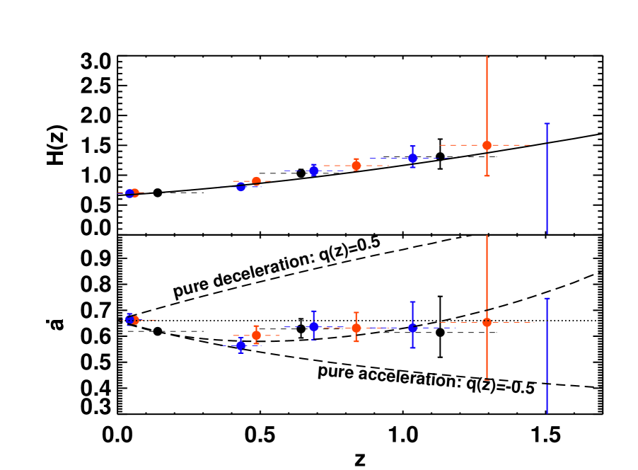
in terms of a conformal or comoving time defined by $a(t)d\eta:=dt$. This conformal flatness makes light propagate, in every comoving frame, as in Minkowski space, so that the kinematic (geometric) quantities in Table I are observables. Assuming the equation of state $w\geq-1$, the Weak Energy Condition $\rho+P\geq 0$ on matter excluding phantom energy in GR, there is no cosmological Big Rip and the inflationary de Sitter universe $a(t)\sim\exp{H_{dS}t}$ is an attractor for expanding RW universes. The Hubble time then grows continuously: $\epsilon_{H}:=dH^{-1}/dt=d\mathcal{H}^{-1}/d\eta+1>0$. But, if the comoving Hubble expansion rate reaches a minimum, $w$ falls below $-1/3$, the deceleration $q:=(1+3w)/2=d(1/\mathcal{H})/d\eta$ becomes acceleration, and the comoving Hubble expansion rate starts increasing with comoving time $d\mathcal{H}/d\eta>0$. This change from deceleration to acceleration (inflation) happened in the very early universe and again recently at $z\sim 1/2$ (Figure 1). While early inflation proceeded until the parameter $\epsilon_{H}\ll 1$, the current inflation started only recently, so that, although $\epsilon_{H}<1$, it does not yet deserve the appellation ”slow-roll parameter”.

Table 1: Kinematic observables for any RW geometry, in terms of Hubble expansion rate $H:=d\ln{a}/dt$ and comoving expansion rate $\mathcal{H}:=da/dt$.

Description	Definition
Hubble time	$H^{-1}:=dt/dN,\qquad N:=\ln{a}$
comoving Hubble time	$\mathcal{H}^{-1}:=1/aH=d\eta/dN$
expansion rate of Hubble time	$\epsilon_{H}:=dH^{-1}/dt=-d\ln{H}/dN=1-d\ln{\mathcal{H}}/dN=1+q$
cosmological stiffness	$\gamma(z):=1+w(z):=-d\ln{H^{2}}/3dN:=-2\dot{H}/3H^{2}:=2\epsilon_{H}/3$
space expansion	$da^{3}/a^{3}=3dN=-d\ln{(1+z)^{3}}=3Hdt=3\mathcal{H}d\eta$
comoving time since Big Bang	$\eta(z):=\int_{0}^{t}dt^{\prime}/a(t^{\prime})=\int_{z}^{\infty}dz^{\prime}/H(z^{\prime})$
proper motion distance back to redshift z	$d_{M}(z)=c\int_{0}^{z}dz^{\prime}/H(z^{\prime})=c(\eta_{0}-\eta(z))$
deceleration	$\ddot{a}/a=H^{2}+\dot{H},\qquad q:=-\ddot{a}/aH^{2}=dH^{-1}/dt-1=d(1/\mathcal{H})/d\eta$
cosmological jerk	$\dddot{a}/a=H^{3}+3H\dot{H}+\ddot{H},\qquad j:=\dddot{a}/aH^{3}=1+3\dot{H}/H^{2}+\ddot{H}/H^{3}$
spacetime (Ricci) curvature	$R:=6(k/a^{2}+\dot{H}+2H^{2})=6(k/a^{2}+(\dot{a}/a)^{2}+\ddot{a}/a)=6(k/a^{2}+H^{2}(1-q))$

II.2 Dynamics: General Relativity or Modified Gravity

In any metric theory, the spacetime curvature (Riemann tensor) would be determined by the matter stress-energy distribution. But, in a Robertson-Walker universe, conformal flatness implies that all of the Riemann curvature tensor depends only on derivatives of the Ricci tensor $R_{\mu\nu}$ and ultimately only on the Ricci spacetime curvature scalar. The only gravitational degrees of freedom are those directly connected to matter through the Ricci tensor, which is subject to four differential Bianchi identities $\nabla^{\mu}R_{\mu\nu}\equiv\nabla_{\nu}R$, following from general covariance and reducing to six the number of degrees of freedom in $R_{\mu\nu}$ and $g_{\mu\nu}$. Besides the metric $g_{\mu\nu}$, the Einstein tensor $G_{\mu\nu}:=R_{\mu\nu}-g_{\mu\nu}R/2$ is the only covariantly conserved second rank tensor This does suggests, but does not require, making $G_{\mu\nu}+\Lambda g_{\mu\nu}$ proportional to the matter tensor $T_{\mu\nu}$.

Now, the Hubble expansion rate $H(t)$ derives from the gravitational field equations:

In Einstein’s original General Relativity, the field equations were

$$G_{\mu\nu}=\varkappa^{2}T_{\mu\nu},\qquad\varkappa^{2}:=8\pi G_{N}:=M_{P}^{-2},$$ (3)

where $G_{N}$ is Newton’s constant, and $M_{P}$ is the reduced Planck mass. In RW cosmology, there is only one independent field equation, leading to the Friedmann-Robertson-Walker equation

$$H(a)^{2}:=\dot{a}^{2}/a^{2}=\varkappa^{2}\rho_{m}/3-k/a^{2},$$ (4)

where $\rho_{m}$ is the material energy density, which vanishes in empty space. The vacuum spacetime curvature $R_{dS}=0$.

In Einstein-Lema$\hat{i}$itre General Relativity, the field equations become

$$G_{\mu\nu}+\Lambda g_{\mu\nu}=\varkappa^{2}T_{\mu\nu}$$ (5)

and the Friedmann-Robertson-Walker equation, the de Sitter radius, and the vacuum spacetime curvature become

$$H(a)^{2}:=\dot{a}^{2}/a^{2}=(\varkappa^{2}\rho_{m}+\Lambda)/3-k/a^{2},\qquad H_{dS}^{-1}=\sqrt{3/\Lambda},\qquad R_{dS}=4\Lambda.$$ (6)

For both the original Einstein and the later Einstein-Lema$\hat{i}$itre field equations, the linearity in $G_{\mu\nu}$ guarantees local conservation of matter stress-energy $T_{\mu\nu}$, and the Friedmann-Robertson-Walker equation as their entire content. $H(t)$ is the only degree of freedom, only the tensor components of the metric $g_{\mu\nu}$ are propagating, and the Weak Equivalence Principle is satisfied.

In Alternative Gravitational Theories, $T_{\mu\nu}$ is no longer proportional to the Einstein tensor, the Bianchi identities no longer imply local conservation of matter stress-energy and the modified Friedmann equation now incorporates only one of the independent field equations. $\dot{H}$ and $\ddot{H}$ become additional degrees of freedom, coupling non-minimally to matter, so that the Weak Equivalence Principle and Newtonian inverse square gravity may no longer be satisfied at short distances.

$H^{2}$ is linear in the matter energy density $\rho_{m}$ in GR, non-linear in modified GR.

The important difference between spacetime and spatial curvature $k$ is illustrated in the two empty stationary RW cosmologies: The flat de Sitter model has $k=0$, but a constant spacetime curvature $R=4\Lambda$ and expansion rate $H_{dS}=\sqrt{\Lambda/3}$. The Milne model $H(a)^{2}=1/a^{2}$ has negative spatial curvature $k=-1$, but vanishing spacetime curvature. The scale is expanding uniformly $\mathcal{H}=\dot{a}=1$, so that Hubble’s original linear relationship between redshift and distance remains exact at all redshifts.

The RW symmetry is broken at small cosmological scales, where inhomogeneities appear. These inhomogeneities or fluctuations break translational invariance, leading to Goldstone mode sound waves and the growth of structure (Section V). This symmetry-breaking at low temperatures and small cosmological scales is reminiscent of symmetry-breaking at low energies in condensed matter and particle physics, except that cosmological structures are gravitationally unstable and will collapse or decay away in an expanding universe.

II.3 ‘Dark energy’ and ‘Equation of State’ Only Describe the Homogeneous Expansion

The expansion history does not determine the dynamics. Although flat Robertson-Walker kinematics does not assume General Relativity, by defining

$$\rho_{DE}:=3M_{P}^{2}H^{2}-\rho_{m},\qquad w_{DE}(z):=-d\ln{(\rho_{DE}/(1+z)^{3})}/3dN,$$ (7)

the homogeneous expansion history may be parameterized by a two-component perfect fluid:

composite mass density:

$\rho:=3M_{P}^{2}H^{2}:=\rho_{m}+\rho_{DE}$

composite pressure:

$P:=-M_{P}^{2}c^{2}(3H^{2}+2\dot{H}):=P_{m}+P_{DE}$

composite enthalpy density:

$\rho+P/c^{2}:=-2M_{P}^{2}\dot{H}=-d\rho/3dN$

composite fluid stiffness:

$\gamma(z):=-d\ln{\rho}/3dN:=1+w=-2\dot{H}/3H^{2}=\gamma_{m}\Omega_{m}+\gamma_{DE}(1-\Omega_{m})$

composite ‘equation of state’:

$w(z):=-(3H^{2}+2\dot{H})/3H^{2}=d\ln{(H^{2}/(1+z)^{3})}/3dN=w_{m}\Omega_{m}+w_{DE}(1-\Omega_{m})$

adiabatic sound speed:

$c_{a}^{2}:=dP/d\rho:=-(1+\ddot{H}/3H\dot{H})$.

Integrating $\gamma_{DE}(z)$, $\rho_{DE}(z)=\rho_{DE0}(1+z)^{3\overline{\gamma_{DE}(z)})}$, where $\overline{\gamma_{DE}}(z):=(1/N)\int_{0}^{N}\gamma_{DE}(N^{\prime})\,dN^{\prime}$ is the past-averaged value of the ’dark energy stiffness’, so that the observed Hubble expansion

$$(H/H_{0})^{2}=\Omega_{m0}(1+z)^{3}+(1-\Omega_{m0})(1+z)^{3\overline{\gamma_{DE}(z)})}.$$ (8)

The departure from homologous expansion, or the curvature in the Hubble expansion rate $\mathcal{H}$ (Figure 1) signals the appearance of ’dark energy’. The present acceleration requires $\gamma_{DE0}<2/3$, so that the ‘dark energy’ is diluting slower than the matter density.

Apparently, after a high-curvature early inflationary phase, our universe expanded monotonically through radiation-dominated and matter-dominated phases, towards a different low-curvature late inflationary phase. During each of the four barotropic phases in Table II, the equation of state, adiabatic sound speed, acceleration, and jerk were constant and the universe expanded homologously towards smaller spacetime curvature. During phase transitions that mix these perfect fluids or introducing cosmological scalar fields, the ‘equation of state’ changes, the composite fluid is imperfect, entropy is generated, and the expansion is no longer simply homologous. Assuming no phantoms intervene to make $w<-1$, the universe will asymptote monotonically towards a future de Sitter phase of small, but finite, spacetime curvature $R_{dS}$.

Table 2: Five barotropic phases of our flat universe expanding homologously as $a\sim t^{1/\epsilon_{H}}$ or $a\sim\exp{Ht}$, with constant equation of state $w=\gamma-1=2\epsilon_{H}/3-1$.

$\gamma$	w	$a(t)\sim t^{1/\epsilon_{H}}$	H(t)$\sim 1/\epsilon_{H}t$	q(t)$=(1+3w)/2$	j(t)$=1+9w(1+w)/2$	$R(t)=6H^{2}(1-q)$	Model Flat Universe
4/3	1/3	$t^{1/2}$	1/2t	1	3	0	radiation-dominated
1	0	$t^{2/3}$	2/3t	1/2	1	$3H^{2}$	matter-dominated (E-dS)
2/3	-1/3	t	1/t	0	0	$6H^{2}$	coasting
1/3	-2/3	$t^{2}$	2/t	-1/2	0	$9H^{2}$	accelerating
0	-1	$\exp{H_{dS}t}$	$H_{dS}=const$	-1	1	$12H_{dS}^{2}=4\Lambda$	inflationary (de Sitter)

The bottom of Figure 1, from Riess et al. Riess et al. (2007), shows the comoving Hubble expansion rate $\mathcal{H}=0.68(1+z)^{q}$ for three hypothetical phases with constant deceleration $q(z)=0.5$ (upper dashed curve), constant acceleration $q(z)=-0.5$ (lower dashed curve)and coasting $q(z)=0$ (central dotted line). The supernova data is fitted by the central dashed curve $q(z)=-0.6+1.2z$, changing from deceleration to acceleration around $z=0.46$ when the comoving expansion rate reached a broad minimum $\mathcal{H}(z)\sim 0.6$.

Figure 1: Upper panel: Hubble expansion rate, in units of 100 km/sec/Mpc, derived from the supernova Gold sample, compared with the Concordance Model with $\Omega_{m0}=0.29,~{}\Omega_{\Lambda}=0.71$, for which acceleration starts at $z\sim 0.7$. Lower panel: Conformal Hubble expansion rate $\mathcal{H}=\dot{a}=H(z)/(1+z)$, compared to constant deceleration model $q(z)=0.5$ (top dashed curve), coasting model $q(z)=0$ (middle dotted curve), constant acceleration model $q(z)=-0.5$ (bottom dashed curve). The Gold data favors the recently accelerating model $q(z)\approx-0.6+1.2z$ (middle dashed curve), with acceleration starting at $z\sim 1/2$ (from Riess et al. Riess et al. (2007), Figure 7).

II.4 ’Dark energy’ is Now Static or Very Nearly Static

By definition, $\rho_{DE}(z)$ and $w_{DE}(z)$ simply summarize ’dark energy’ and its evolution. This ’dark energy’ is either a newly-revealed material constituent within GR or a modification to GR:

Dark Energy:

In Einstein’s original General Relativity, the total matter stress-energy is covariantly conserved and Friedmann equation (4) is the only independent field equation. For a given form of kinetic energy, $\dot{\phi}$ lets the field $\phi(t)$ substitute for the time. If the scalar field is canonical (quintessence), with kinetic energy density $\partial_{\mu}{\phi}\partial^{\mu}{\phi}/2:=X/2$, then $\dot{\phi}^{2}=(1+w_{DE})\rho_{DE}$ and the potential energy density $V(\phi)=(1-w_{DE})\rho_{DE}/2=(1-w_{DE})(3M_{P}^{2}H^{2}-\rho_{m})/2$, so that the expansion history determines the quintessence potential. If the scalar field is non-canonical (tachyonic), the kinetic energy is non-linear in $X$ and $w_{DE}$ determines a different potential.

Dark Gravity:

If no such Dark Energy exists, then $w_{DE}(z):=w(z)/(1-\Omega_{m}(z))$ expresses the Dark Gravity modification to the Friedmann equation. The simplest form of Dark Gravity is the static Cosmological Constant Model, for which $\rho_{DE}=const,~{}w_{DE}=-1$. If Dark Gravity is dynamic, then the modified Friedmann equation is only one of the field equations

Dynamical Dark Gravity or Dark Energy introduce scalar fields non-minimally or minimally coupled to gravity. The new scalar fields appear as negative pressure matter in Dark Energy, or as new gravitational scalar degrees of freedom in Dark Gravity i.e. the Friedmann equation (4) is modified on the left side or on the right side.

According to WMAP3 Spergel et al. (2006), the present Hubble expansion rate $H_{0}=\mathcal{H}_{0}=73\pm 3~{}km/sec/Mpc$, Hubble time $H_{0}^{-1}=\mathcal{H}_{0}^{-1}=13.4\pm 0.5~{}Gyr=4.11\pm 0.17~{}Gpc$, so that the cosmic acceleration has only increased to $-q_{0}\approx 0.52$, the ”slow-roll” parameter has only decreased to $\epsilon_{H0}=0.48$, the overall ‘equation of state’ is now $w_{0}\approx-0.74$. For spatially flat $\Lambda CDM$, the SNLS supernova data then implies $\Omega_{m0}=0.234\pm 0.035$ and the ‘dark energy equation of state’ $w_{DE0}=-0.926^{+0.051}_{-0.075}$ Spergel et al. (2006). This limit to how dynamical the ’dark energy equation of state’ can now be will improve still more, when more weak lensing measurements of galaxy halo masses and cluster abundances lead to an improved constraint on the matter spectrum amplitude $\sigma_{8}$ Rozo et al. (2007).

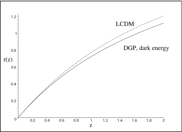
The lower curve in Figure 2, from Koyama and Maartens Koyama and Maartens (2006), shows the Dark Gravity/Dark Energy degeneracy in DGP comoving distance $d_{M}(z)$ derived from the DGP expansion history. In Section V, we will see how this Dark Energy/Dark Matter degeneracy in the homogeneous evolution may be resolved by prospective observations of the growth of inhomogeneities.

Figure 2: The comoving or proper motion distance $r(z)\equiv d_{M}(z):=c\int_{0}^{z}dz^{\prime}/H(z^{\prime})$ back to redshift $z$, shows curvature at high redshift depending on the cosmological model. Distances obtained from the dynamic DGP Dark Gravity model or its equivalent Dark Energy mimic are somewhat less than those obtained from the static LCDM model because DGP gravity was somewhat stronger in the past. (from Koyama and MaartensKoyama and Maartens (2006)).

III SOME DYNAMICAL CONSEQUENCES OF VACUUM SPACETIME CURVATURE

III.1 Interpretation of Asymptotic Spacetime Curvature As Gravitational Vacuum Energy

We have been at pains to distinguish between kinematics, as observed in the accelerating expansion of our universe, and the dynamics driving this expansion. Nevertheless, Robertson-Walker symmetry has some dynamical consequences, which help elucidate the physical consequences of vacuum spacetime curvature (’gravitational vacuum energy’) and the connection between geometry and material sources. .

In General Relativity, the Bianchi identities assure covariant conservation of the material stress-energy. This will no longer generally be true for Dark Gravity, where the material stress-energy tensor $T_{\mu\nu}$ is no longer simply proportional to $G_{\mu\nu}+\Lambda g_{\mu\nu}$ and not generally locally conserved. Nevertheless, in empty space, the Ricci scalar and the Hubble expansion rate will still asymptote to the small constant values $R_{dS}=4\Lambda$. We will interpret Dark Gravity geometrically, avoiding identifying the vacuum Ricci tensor with any material stress-energy, and avoiding the Cosmological Constant Problem, by tuning the geometry to $\Lambda:=3H_{dS}^{2}=2.19H_{0}^{2}$ or de Sitter radius $H_{dS}^{-1}\sim 5.2~{}Gpc$. Indeed, there is no evidence that quantum vacuum energies gravitate at all: the observed electromagnetic Casimir effect, demonstrates how electromagnetic fields interact with electromagnetic vacuum quantum fluctuations, and may have little to do with the gravitational properties of the vacuum energy Lamoreaux (2007). The Cosmological Constant Problem expresses the inequivalence of the gravitational and material vacua!

The physical significance this ’gravitational vacuum energy’ will now be illustrated by two examples of how vacuum spacetime curvature impacts dynamics.

III.2 Vacuum Curvature Classification of Robertson-Walker Cosmologies

In the absence of Dark Energy, our accelerating universe is now dominated by pressure-free matter and Dark Gravity must modify the Friedmann equation, in the infra-red. Such low-curvature modifications preserve Einstein gravity and the Equivalence Principle locally. Alternatively, Einstein gravity might be modified in the ultra-violet. Such high-curvature modifications require sub-millimeter corrections to Newton’s inverse-square gravity. In this way, the presence or absence of vacuum energy distinguishes low- from high-curvature modifications of General Relativity. While the gravitational vacuum may be intrinsically classical in origin, the high-curvature modifications must involve quantum gravity Arkani-Hamad et al. (1998); Randall and Sundrum (1999); Binutray et al. (2000).

III.3 Vacuum About An Isolated Spherically Symmetric Source

The Riemann curvature tensor can always be decomposed into a traceless part (Weyl or conformal tensor) plus a remaining part (Ricci tensor). In Robertson-Walker cosmologies, the (four-dimensional) Weyl tensor vanishes, the Ricci tensor is determined by the local matter distribution, and the Ricci scalar depends on the acceleration imparted to matter by the field equations. We now consider the opposite extreme, where the the Ricci tensor vanishes or is constant, but the Weyl tensor is determined by the non-local matter sources.

The vacuum energy determines the gravitational field about any isolated spherically symmetric source, without reference to the source other than its mass $M$ or Schwarzschild radius $r_{S}:=2G_{N}M$:

• In General Relativity, the vacuum field equations are the vanishing of the Einstein tensor $G_{\mu\nu}:=R_{\mu\nu}-Rg_{\mu\nu}/2=0$, and the unique spherically symmetric vacuum metric is the Schwarzschild-de Sitter metric

  $$g_{tt}=g_{rr}^{-1}=1-r_{S}/r+\Lambda r^{2}/3.$$ (9)

  A vanishing vacuum energy signifies the Schwarzschild metric: $g_{tt}=g_{rr}^{-1}=1-r_{S}/r$. This is Birkhoff’s Theorem, a generalization of Newton’s Iron Sphere Theorem: for any thin spherical shell, the gravitational potential vanishes inside, and decreases outside as $1/r$. Birkhoff’s clearly geometric theorem expresses the significance of vanishing vacuum energy in Einstein gravity.

• In the Dvali-Gabadadze-Porrati Model, discussed in Appendix C, the field equations are the vanishing of $G_{\mu\nu}+E_{\mu\nu}=0$, where $E_{\mu\nu}$ is the projection of the five-dimensional Weyl tensor onto the four-dimensional brane, whose dynamical importance will be apparent in Figure 3. The DGP vacuum metric is

  $$g_{tt}=1-r_{S}/2r+\sqrt{r_{S}r/2r_{c}^{2}},\quad g_{rr}^{-1}=1+r_{S}/2r-\sqrt{r_{S}r/8r_{c}^{2}},\qquad r\lesssim r_{\star}:=(r_{S}r_{c}^{2})^{1/3},$$ (10)

  where $r_{c}$ is a new cosmological scale. Because this metric differs from the Schwarzschild metric even when $r_{c}\rightarrow\infty$, there are no DGP Iron Sphere or Birkhoff’s Theorems. This emphasizes the characteristic geometric nature of these theorems in General Relativity and the distinctive role of the five-dimensional Weyl tensor in brane cosmology.

In both cases, the vacuum energy modifies the Schwarzschild metric at distances beyond the Vainstain radius $r_{*}:=(r_{S}H_{dS}^{-2})^{1/3}$, where the de Sitter radius $H_{dS}^{-1}$ is $H_{0}^{-1}$ or $r_{c}=\beta H_{0}^{-1}$, for $\Lambda$CDM and for $DGP$ respectively. This geometric mean between $r_{S}$ and $r_{c}^{2}$ will also be where fluctuations start growing according to Friedmann-Lema$\hat{i}$tre or linearized DGP Lue et al. (2004), instead of according to Einstein gravity. These Vainstain scale modifications may potentially be observable in ultra-precise measurements about isolated Sun-like stars ($r_{S}\sim 3~{}km,~{}r_{\star}\sim 280~{}pc$) or spherical galaxy clusters ($r_{S}\sim 100~{}pc,~{}r_{\star}\sim 28~{}Mpc$) Iorio (2005a). Their higher-order effects may also someday be tested in ultra-precise Solar System measurements of anomalous precessions of planetary or lunar orbits Lue and Starkman (2003); Dvali et al. (2003); Sereno and Jetzer (2006a) or of a secular increase in the Astronomical Unit Iorio (2005b).

The homogeneity and isotropy of RW cosmologies implies local isotropy about any point. In a homogeneous universe, what is true locally is true everywhere. Using Birkhoff’s Theorem, Milne and McCrae Milne (1934); McCrea and Milne (1934) were able to derive the Friedmann equation $k/a^{2}+H^{2}=\varkappa^{2}\rho/3$ for a pressure-free universe, from Newtonian gravity, without assuming Einstein’s field equations: In a dust universe, Newtonian cosmology would then have implied the Friedmann equation! (Of course, in Newtonian cosmology, space would always be flat, so that the spatial curvature $k$ and scale factor $a$ would lack the geometrical interpretation GR conveys.) Because vacuum energy is now known to exist, Birkhoff’s Theorem and the Milne-McCrae derivation is today only an historical curiosity.

In summary, without Dark Energy, the accelerating universe requires vacuum spacetime curvature, called gravitational vacuum energy. Besides its cosmological implications, gravitational vacuum energy implies deformation of the Schwarzschild metric about any isolated source at the Vainstain radius $r_{*}$, which is significantly smaller than the de Sitter radius.

IV HOMOGENEOUS EXPANSION MEASURES ONLY KINEMATIC VARIABLES

While realizing that the homogeneous expansion cannot resolve the Dark Energy/Dark Gravity degeneracy, we finally review static and dynamic fits to the observed expansion history.

IV.1 Cosmography: Distances to Supernovae, Luminous Red Galaxies, Last Scattering Surface

For small radial distances and small galaxy recessional velocities, Hubble’s Law $v=cz=H_{0}d$ is a kinematic consequence of RW symmetry, illustrated by the linear region $d=cz/H_{0}$ in Figure 2. But, in curved spacetime, different global distances are defined only by physical observables: the comoving distance back to a source defines the proper motion distance $d_{M}(z):=c(\eta_{0}-\eta(z))$; the observed flux $\mathcal{F}:=\mathcal{L}/4\pi d_{L}^{2}$ from standard candles defines the luminosity distance $d_{L}(z):=\sqrt{4\pi\mathcal{F}/\mathcal{L}}=(1+z)d_{M}$; the angular size $\theta_{A}$ of a standard ruler $r_{s}$ defines the angular diameter distance $d_{A}(z):=r_{s}(z)/\theta_{A}=d_{M}/(1+z)$. These different cosmological distances are observed as follows:

CMB:

The angular diameter distance of the first acoustic CMB peak at the last scattering surface measures the comoving size subtended at angular scale $\theta_{A}$. The measured CMB shift parameter $S:=\sqrt{\Omega_{m0}}H_{0}d_{M}(z_{r})=1.70\pm 0.03$ then determines the distance to the last scattering surface at $z_{ls}=1089$ and a standard ruler, the comoving sound horizon $r_{s}=147.8^{+2.6}_{-2.7}~{}Mpc$ Spergel et al. (2006); Wang and Mukherjee (2006).

BAO:

This provides a standard ruler for measuring the line-of-sight distances $H(z)r_{s}$ to luminous red galaxies (LRG) and their angular size $d_{A}(z)/r_{s}$. From the $z_{1}/z_{ls}$ distance ratio $R_{0.35}=0.0979\pm 0.0036$ and the measured combination $A:=\sqrt{\Omega_{m0}}H_{0}[d_{M}^{2}(z_{1})/z_{1}^{2}H(z_{1})]^{1/3}=0.469\pm 0.017$, Fairbairn and Goobar Fairbairn and Goobar (2006) and Eisenstein et al. Eisenstein et al. (2005) obtain the proper motion distance $d_{M}(z_{1})$ to luminous red galaxies, typically at redshift $z_{1}=0.35$.

SN:

The luminosity distances of calibrated supernovae Ia are derived directly from their observed fluxes Perlmutter et al. (1999); Astier et al. (2006); Miknaitis et al. (2007); Riess et al. (2007). The quality data Astier et al. (2006); Miknaitis et al. (2007); Riess et al. (2007) is now dominated by systematic errors due to nearby velocity structures and dust.

WL:

weak gravitational lensing of the light from galaxy clusters, from the X-ray emission from hot gravitationally confined electrons, and from the upscattering of CMB relict photons by these hot electrons (Sunyaev-Zelovich effect) measures the proper motion distances of these sources and the fluctuation growth factors $g(z)$ at these distances. Weak lensing observations are independent of the baryonic composition of the lenses and enjoy a statistical potential far greater than BAO or SN.

GC:

galaxy clustering also measures both $d_{M}(z)^{2}/H(z)$ and $g(z)$, but is subject to large systematic errors, deriving from their baryonic composition and foreground noise.

The proper distance $c(\eta_{0}-\eta(z)):=d_{M}(z)=(1+z)d_{A}(z)=d_{L}(z)/(1+z)$, must be differentiated with respect to redshift, to obtain the Hubble times $H(z)^{-1}=d\eta/dz,~{}\mathcal{H}^{-1}=d\eta/d\ln{1+z}$. Obtaining the composite ’equation of state’ $w(z)$ and the ’dark energy equation of state’ $w_{DE}(z)=w(z)/(1-\Omega_{m}(z)$, requires a second differentiation of the observed distances. This requires smoothing and binning of the data Wang and Tegmark (2004), smears out information on the ‘equation of state’ Maor et al. (2001), and justifies no more than two- parameter models Linder and Huterer (2005); Caldwell and Linder (2005) in fitting current and currently underway observations. The usual Chevalier-Polarski-Linder parameterization Chevalier and Polarski (2001); Linder (2003) of the ’dark energy equation of state’

$$w_{DE}(z)=w_{0}+w_{a}(1-a),\qquad\overline{w_{DE}(z)}=w_{0}+w_{a}(1-a)\ln{a}$$ (11)

assumes that ’dark energy’ grows smoothly, monotonically and mostly at low redshifts, a prior assumption that will be tested only after more observations at higher redshifts become available. More generally, because observations constrain the directly observable $H(z)$ and the ‘dark energy’ density $\rho_{DE}$ better than its derivative, it might be better to parameterize the past average $\overline{w_{DE}}(z)$, rather than $w_{DE}(z)$ Wang and Freese (2006).

IV.2 Classical Cosmological Constant Model $\Lambda$CDM

Einstein introduced his cosmological constant $\Lambda g_{\mu\nu}$ on the left (geometric) side of his original field equations (5), changing them to the Einstein-Lema$\hat{i}$tre form (5) and changing the original Einstein lagrangian $R$ into the Einstein-Lema$\hat{i}$tre lagrangian $R-2\Lambda$. (Equivalently, the original Einstein lagrangian $R$ can be varied holding $\sqrt{g}=-1$. In this unimodular gravity approach Buchmuller and Dragon (1988); Unruh (1989), $\Lambda$ does not appear in the lagrangian, but as an undetermined c-number (!) Lagrange multiplier. This approach stresses the classical nature of the cosmological constant.)

The alternative Dark Matter interpretation subtracts $\Lambda g_{\mu\nu}$ from the right side of equation (9) and interprets the cosmological constant as a constant-density fluid with $\rho_{vac}:=M_{P}^{2}\Lambda=(2.39~{}meV)^{4}$. These two interpretations of the cosmological constant already exhibit the Dark Gravity/Dark Energy degeneracy in expansion history. Although we would prefer to stress the geometric nature of $\Lambda$ as intrinsic spacetime curvature, we will conform to established parlance by calling it ’vacuum energy’.

Allowing for possible space curvature, the Friedmann equation (6) contains two parameters, $\Lambda$ and the present energy density $\rho_{m0}$, which is now almost completely that of non-relativistic matter (dust). In units of the present critical density $\rho_{cr0}:=3M_{P}^{2}H_{0}^{2}$,

$$(H/H_{0})^{2}=\Omega_{m0}(1+z)^{3}+\Omega_{\Lambda 0}+\Omega_{K0},\qquad\Omega_{m0}+\Omega_{\Lambda 0}+\Omega_{K0}\equiv 1,$$ (12)

where $\Omega_{m0},\Omega_{\Lambda 0}$, are the present matter and vacuum fractions. Measuring only the homogeneous expansion cannot resolve this historic static Dark Gravity/Dark Energy degeneracy. We will now see how this degeneracy persists, even if the ’dark energy’ is made dynamic.

IV.3 Dynamical Cosmological Models

The static Cosmological Constant Model can be made dynamic, by introducing additional parameters relaxing the condition . Dynamical models allow the vacuum energy to decay down to its present observed value, no model explains the Cosmic Coincidence, why we are observing the universe now, when the present matter density $\rho_{m0}\sim\rho_{vac}/3$. The answer to this question must involve the observers’ role in cosmology (Section VII.B).

Table III, derived from Davis et al.Davis et al. (2007), tabulates twelve ‘dark energy’ fits to the SN+CMB+BAO homogeneous evolution data, ordered according to the Schwarz Bayes Information Criterion (BIC), an approximation to the marginal likelihood of improving the fit by adding more parameters, which measures the strength of each model in giving the best fit with the fewest parameters. Although some of these fits derive from interesting Dark Gravity models, their homogeneous evolution can always be mimicked by equivalent Dark Energy models.

The first eight of these twelve models fit the combined data almost equally well. But, ordered by BIC, the twelve models fall into four categories of increasing complexity:

1. The Flat Cosmological Model, the simplest one-parameter fit to the combined SN+BAO+CMB data, appears on the top row of Table III. In this model, cosmic acceleration started at $z_{acc}=0.76\pm 0.010,~{}6.7\pm 0.4$ Gyr ago, but the the cosmological constant began dominating over ordinary CDM only later at $z_{eq}=0.40\pm 0.04,~{}4.3$ Gyr ago Melchiorri et al. (2007). (All confidence limits are 95%.). This ‘static dark energy‘ model, with $w_{DE}=-1$, serves as a standard for comparison with the following eleven dynamical models.

2. The next three models are spatially curved cosmological constant, spatially flat constant $w_{DE}$, and flat generalized Chaplygin gas, for which models,

   $$P=-A/\rho_{DE}^{\alpha},\quad(H(z)/H_{0})^{2}=[A+(1-A)(1+z)^{3(1+\alpha)}]^{1/(1+\alpha)},\quad A^{1/(1+\alpha)}=\Omega_{\Lambda 0}=1-\Omega_{m0}$$ (13)

   introduce a second parameter, without any significant loss in GoF. The broad uncertainties in the second parameter show the insignificance of going beyond the simple one-parameter Flat Cosmological Constant model. In the constant $w_{DE}$ model, cosmic acceleration started at $z_{acc}=0.81\pm 0.30,~{}6.8\pm 1.4$ Gyr ago, but the the cosmological constant began dominating over ordinary CDM only at $z_{eq}=0.44\pm 0.20,~{}4.5\pm 1.0$ Gyr ago, slightly sooner than in $\Lambda$CDM Melchiorri et al. (2007).

3. The next four models listed are the variable $w_{DE}(z)$, spatially curved constant $w_{DE}$, generalized Chaplygin gas

   $$P=-A/\rho_{DE}^{\alpha},\quad(H(z)/H_{0})^{2}=\Omega_{K0}(1+z)^{3}+(1-\Omega_{K0})[A+(1-A)(1+z)^{3(1+\alpha)}]^{1/(1+\alpha)},$$ (14)

   and flat, matter-dominated modified Cardassian polytropic Gondolo and Freese (2003), which expands according to the modified Friedmann equation

   $$(H/H_{0})^{2}=\Omega_{m0}(1+z)^{3}[1+(\Omega_{m0}^{-q}-1)(1+z)^{3q(n-1)}]^{1/q}.$$ (15)

   These four models introduce a third parameter, with insignificant loss in GoF, but at the price of still more complexity.

4. The last four models listed are the spatially flat or curved ordinary Chaplygin gas and DGP models (17) discussed in Section VI and Appendix C. The flat models depend on only the one parameter $\Omega_{m0}\approx 0.27$, for which, in the DGP case, $\beta\approx 1.4,~{}r_{c}\sim 5.7~{}Gpc$. The spatially-curved DGP model requires $\Omega_{m0}=0.27\pm 0.03,\Omega_{K0}=0.13\pm 0.05$ These original DGP models cannot simultaneously fit the SN+BAO and CMB data Fairbairn and Goobar (2006) and have poor $GoF\approx 20\%$. The two ordinary Chaplygin models simply do not fit all the data. (Ignoring the BAO and CMB data, Szydlowski et al. Szydlowski et al. (2006) reached the opposite conclusion.) All four DGP and ordinary Chaplygin gas models show too rapid variation of $H(z)$ and are rejected by their poor GoF.

Table 3: Classical cosmological constant and dynamical models for the homogeneous evolution. The goodness of fit (GoF) approximates the probability of finding a worse fit to the data. The Bayes Information Criteria BIC prefer the one-parameter Flat Cosmological Constant Model. The $\Delta$BIC values for the other two- and three-parameter models are then measured with respect to this Flat Cosmological Constant Model. The table is derived from Davis et al. Davis et al. (2007), Table 2, ordered by increasing complexity $\Delta$BIC, but with some additions to the last column.

Model	$\chi^{2}$/dof	GoF(%)	$\Delta$BIC	Parameters Fitted
Flat Cosmologic Constant	194.5 / 192	43.7	0	$\Omega_{m0}=0.27\pm 0.04$
Flat Generalized Chaplygin Gas (13)	193.9 / 191	42.7	5	$A=0.73\pm 0.05,~{}\alpha=0.06\pm 0.10$
Cosmological Constant (12)	194.3 / 191	42.0	5	$\Omega_{m0},\Omega_{\Lambda 0}$
Flat constant EOS $w_{DE}$	194.5 / 191	41.7	5	$\Omega_{m0}=0.27\pm 0.04,~{}w_{DE}=-1.01\pm 0.15$
Flat variable $w_{DE}(z)$ (11)	193.8 / 190	41.0	10	$\Omega_{m0}=0.27\pm 0.04,~{}w_{0}=-1.0\pm 0.4,~{}w_{a}=-0.4\pm 1.8$
Spatially-curved constant $w_{DE}$	193.9 / 190	40.8	10	$\Omega_{m0},~{}w_{DE},~{}\Omega_{\Lambda}$
Generalized Chaplygin Gas (14)	193.9 / 190	40.7	10	$A,\alpha,\Omega_{K0}$
Cardassian Polytropic (15)	194.1 / 190	40.4	10	$\Omega_{m0},q,n$
Flat Dvali-Gabadadze-Porrati (17)	210.1 / 192	17.6	14	$\Omega_{m0}\approx 0.27$
Dvali-Gabadadze-Porrati (17)	207.4 / 191	19.8	18	$\Omega_{m0}=0.27\pm 0.05,~{}\Omega_{K0}=0.13\pm 0.02$
Ordinary Chaplygin Gas (14,$\alpha=1$)	220.4 / 191	7.1	30	$A,~{}\Omega_{K0}$
Flat Ordinary Chaplygin Gas (13,$\alpha=1$)	301.0 / 192	0.0	30	$A$

Acceptable models all agree at low redshift and are now static or quasi-static. Table III excludes fast evolution, such as would be predicted by many Dark Gravity models. For example, in Figure 2 Koyama and Maartens (2006), the slopes $d_{M}/dz=H(z)^{-1}$ show that the too-dynamic ordinary DGP model would predict expansion rates, that already at $z=2$, evolve about $10\%$ faster than those obtained from the static Classical Cosmological Constant Model.

The simplest and best fit to all the combined is the Flat Cosmological Constant Model on the first line of Table III. The remaining seven acceptable quasi-static models on lines 2-8 of Table III, with essentially the same GoF as $\Lambda CDM$, have their additional parameters so poorly constrained so that, in the worst cases, Davis et al. Davis et al. (2007) did not quote their values. These complex models, with more parameters, will only be tested after much more high redshift supernova or weak lenses are observed Riess et al. (2007). Although no evidence requires any dynamical model for ’dark energy’, until these seven models are excluded observationally, we will go on to study possible dynamical manifestations of gravitational vacuum energy.

V GROWTH OF FLUCTUATIONS CAN DISTINGUISH COSMODYNAMICS

Dynamical ’dark energy’ has two distinct effects: it alters the homogeneous evolution $H(z)$, as already discussed, and it alters the growth of fluctuations through the fluctuation growth factor, which we now discuss.

V.1 Dark Energy: Canonical and Non-canonical Scalar Fields (Quintessence and K-essence)

Dark Energy and its alternatives are reviewed in Albrecht et al. (2006); Padmanabhan (2005) and ten model fits to the expansion history, with and without spatial curvature and cosmological constant, are tabulated by Szydlowski et al. (2006). If Dark Energy exists, it is usually attributed to an additional ultra-light scalar field $\phi$ with lagrangian $\mathcal{L}(\phi,X)$, where $X:=\partial_{\mu}{\phi}\partial^{\mu}{\phi}$. The pressure, energy density, ‘equation of state’, and adiabatic sound speed are then $P=\mathcal{L},~{}\rho=2X\mathcal{L}_{,X}-\mathcal{L},~{}w=P/(2XP_{,X}-P),~{}c_{a}^{2}:=dP/d\rho$ respectively. The lagrangian $\mathcal{L}$ is canonical (quintessence) or non-canonical (k-essence) according to whether the kinetic energy is linear or not in $X$:

Quintessence

is driven by a slow-rolling scalar potential that can be tuned to track the radiation/matter until it now dominates, with ’equation of state’ now decreasing $dw_{DE}/dz>0$. In any canonical scalar field, inhomogeneities will propagate with an effective sound speed $c_{s}^{2}=1$.

K-essence

is kinetic energy driven, can be chosen to track only the radiation energy density, so that, after radiation/matter equality, k-essence can start dominating over ordinary matter. The $w_{DE}$ dropped sharply near matter/radiation equality and has been increasing thereafter $dw_{DE}/dz<0$. K-essence apparently cannot arise as a low-energy effective field theory of a causal quantum field theory Bonvin et al. (2006).

Dynamical Dark Energy was originally invoked to make a material vacuum energy decay down to the present small value $\rho_{vac0}\sim 2M_{P}^{2}H_{0}^{2}\lll M_{P}^{4}$ or small expansion rate $H_{0}^{2}\lll M_{P}^{2}$. Both kinds of Dark Energy ultimately require fine-tuning in different ways: quintessence, in order to make tracing stop before now; k-essence, in order to initiate the transition towards dominance in the matter-dominated epoch. Because these scalar fields are non-renormalizable and fundamentally unnatural, both need to be interpreted as ad hoc low-energy effective field theories.

V.2 Entropic Fluctuations Determine the Growth Factor

In a mixture of cosmological fluids or with dynamical scalar fields, the ‘equation of state’ is generally not adiabatic: fluctuations propagate with an effective sound speed squared $c_{s}^{2}:=P_{,X}/\rho_{,X}=(1+2(P_{,XX}/P_{,X})X)^{-1}$, which equals unity only in a canonical field theory. The entropic pressure fluctuations are proportional to $(1+w)(c_{s}^{2}-c_{a}^{2})$, so that in the quasi-static limit $w(z)\sim-1$, they are small and insensitive to the effective sound speed. This minimizes the differences between static and dynamic Dark Energy fluctuation growth factors that we would like to distinguish.

How different microscopic dynamics and different effective sound speeds can underly the same Dark Energy ‘equation of state’ is illustrated by the original Chaplygin gas Bento et al. (2005), whose adiabatic ‘equation of state’ $P(\rho)=-A/\rho$ and adiabatic sound speed $c_{a}^{2}=-P/\rho=-w(z)$. This equation of state can be derived from either a non-canonical or a canonical scalar field. If derived from the constant potential Born-Infeld Lagrangian $\mathcal{L}=-V_{0}\sqrt{1+\varkappa^{2}X}$, with non-canonical $\rho=V_{0}/\sqrt{1-\varkappa^{2}X},~{}P=-V_{0}\sqrt{1-\varkappa^{2}X},~{}V_{0}^{2}\equiv A$, the fluctuations remain adiabatic, and the effective sound speed $c_{s}^{2}=c_{a}^{2}=-w(z)$. But, if derived from the canonical scalar field with potential $V(\phi)=(\sqrt{A}/2)[\cosh{3\phi}+1/\cosh{3\phi}]$ Bento et al. (2005), entropic fluctuations make the effective sound speed $c_{s}^{2}=1\neq c_{a}^{2}$. These canonical and non-canonical Chaplygin gas models give the same adiabatic sound speed $c_{a}^{2}=-w(z)$, but different effective sound speeds, $c_{s}^{2}=1,~{}-w(z)$ respectively, and different fluctuation growth factors. (As mentioned in Section IV.C, this original Chaplygin gas does not fit the observed expansion history, but can be generalized to $P=-A/\rho^{\alpha},~{}c_{a}^{2}=-\alpha w,~{}\alpha=0.06\pm 0.10$, which is indistinguishable from $\Lambda CDM$ and fits very well Amendola et al. (2003); Bento et al. (2005); Zhu (2004).)

VI MODIFIED GRAVITY: DVALI-GABADADZE-PORRATI BRANE COSMOLOGY

Because Dark Energy is contrived, requires fine tuning and cannot be directly detected in the laboratory or solar system, we now turn to Dark Gravity as the alternative dynamical source of cosmological acceleration. These Dark Gravity alternatives, classified in the Appendix, arise naturally in braneworld theories, naturally incorporate a small spacetime intrinsic curvature, and may unify ‘dark energy’ and dark matter, and early and late inflation. While fitted to the observed cosmological acceleration, they may also ultimately be tested in the solar system, Galaxy or galaxy clusters Lue and Starkman (2003); Iorio (2005a, b); Lue (2006); Sereno and Jetzer (2006a).

In the self-accelerating solution of the original DGP model Dvali et al. (2000); Deffayet (2001); Deffayet et al. (2002), discussed in Appendix C, gravity leaks into the five-dimensional bulk at cosmological scales greater than $r_{c}$, weakening gravity on the four-dimensional brane. This leads to a four-dimensional Friedmann equation

$$H^{2}+k/a^{2}-H/r_{c}=\varkappa^{2}\rho/3.$$ (16)

Defining $\beta:=r_{c}H_{0}$, which can be written as

$$(H(z)/H_{0})^{2}=[1/2\beta+\sqrt{(1/2\beta)^{2}+\Omega_{m0}(1+z)^{3}}]^{2}+\Omega_{K0}(1+z)^{2},1\equiv\Omega_{m0}+\Omega_{K0}+\sqrt{1-\Omega_{K0}}/\beta,$$ (17)

interpolating between a past matter-dominated universe and a future de Sitter universe.

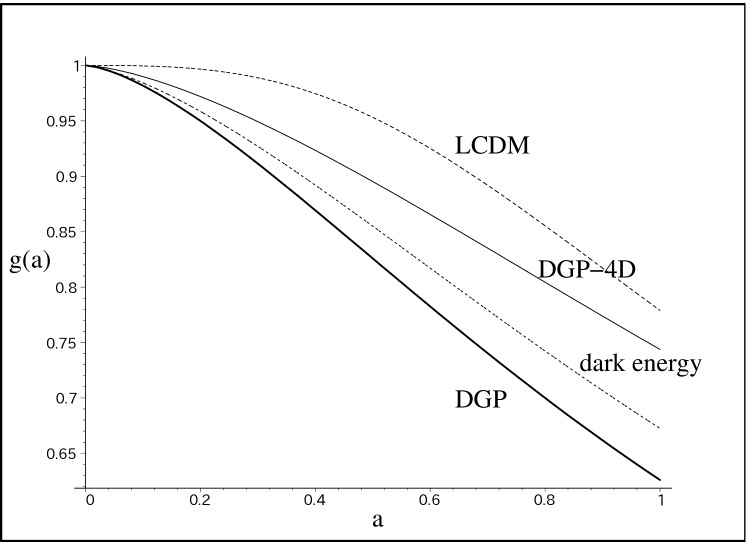
Fig. 3 shows the growth factors in this DGP Dark Gravity and its Dark Energy mimic both evolving substantially faster than in the Cosmological Constant Model $\Lambda CDM$. This figure also shows a relatively smaller difference between Dark Gravity DGP and its Dark Energy mimic. In the next decade, weak lensing observations may distinguish between static and dynamic ’dark energy’, but not between Dark Gravity and Dark Energy.

As discussed in Section IV.C, the original DGP models cannot simultaneously fit the SN+BAO and the CMB data. We have used these models only to suggest the importance of the 5D Weyl tensor in any braneworld dynamics and to illustrate how dynamics is better tested in the growth of fluctuations (Figure 3) than in the homogeneous expansion history (Figure 2). In any realistic model, because the evolution is, at most, quasi-static, any dynamical effects on the growth of fluctuations will be minimal, and will be best studied in the weak lensing convergence of light from galaxies at $0<z<5$, from neutral hydrogen at $6<z<20$, and ultimately from the CMB last scattering surface at z=1089 Albrecht et al. (2006); Ishak et al. (2006). Galaxy clustering also measures $g(z)$, but requires large corrections for baryonic composition and foreground noise to reduce their large systematic errors.

Figure 3: The linear growth history $g(a):=\delta/a$ for flat $\Lambda$CDM (long dashed), DGP Dark Gravity (thick solid) and Dark Energy (short dashed) models in Fig. 2. DGP-4D (thin solid) shows the incorrect result that would be obtained by neglecting perturbations of the DGP 5D Weyl tensor. The 5D Weyl tensor perturbations thus distinguish the static Dark Energy model from the two dynamical Dark Gravity and mimicking Dark Energy models. In the DGP Dark Gravity model, Newton’s ‘constant’ weakens with time, so that its growth suppression evolves even faster than in its mimicking Dark Energy model. (from Koyama and Maartens (2006) ).

VII COSMOLOGICAL CONSTANT, FINE-TUNED DARK ENERGY, OR MODIFIED GRAVITY?

VII.1 Phenomenological Conclusions: Vacuum Energy is Now Static or Quasi-static

We have reviewed present and prospective observations of ’dark energy’, in order to emphasize the differences between kinematical and dynamical observations, between static and dynamic ‘dark energy’, and between Dark Energy and Dark Gravity. We conclude:

• Cosmological acceleration is explicable by either a small fine-tuned cosmological constant or by ‘dark energy’, which is now nearly static. If dynamic, this ‘dark energy’ is either an additional, ultra-light negative pressure material within General Relativity, or a low-curvature modification of Einstein’s field equations.

• The simplest and best fit to the expansion history, the Classical Cosmological Constant Model, interprets ’dark energy’ as a classical intrinsic spacetime curvature, giving geometric structure to empty space. This classical interpretation distinguishes ’gravitational vacuum energy’ from the ground state of quantum matter, and renounces any attempt to explain its small value as a quantum vacuum energy.

• The observed homogeneous expansion history may also be fitted by ‘dark energy’ decaying from its huge primordial value and now nearly static. This static or quasi-static ’dark energy’ presently observed, whether Dark Energy or Dark Gravity requires fine-tuning.

• The inhomogeneity growth rate potentially distinguishes between static and dynamic ‘dark energy’ and between Dark Energy and Dark Gravity. Because the ’dark energy’ is now static or nearly static, differences in the large-scale angular power spectrum, mass power spectrum, or gravitational weak lensing Hockstra et al. (2006) will be small, but may distinguish static from dynamic ‘dark energy’. Distinguishing between Dark Energy and Dark Gravity will remain more problematic.

• No model yet explains the Cosmological Constant Problem, why quantum vacuum energies apparently do not gravitate. Nor does any model explain the Cosmic Coincidence, why we observers live at a time when the matter and vacuum energy densities are comparable.

Low-curvature modifications of Einstein gravity are conceptually less contrived than fine-tuned Dark Energy, explain cosmological acceleration as a natural consequence of geometry, and may unify early and late inflation. Geometric modifications may be intrinsic in four dimensions, or may arise naturally in braneworld theories. Invoked in the first place to explain recent cosmological acceleration, these low-curvature modifications of Einstein gravity may even be testable by refined solar system or galaxy observations. The outstanding problem in both Dark Energy or Dark Gravity remains the significance of the Cosmic Coincidence, which (unless it is fine-tuned), clearly refers to the role of conscious observers.

VII.2 Metaphysical Conclusions: The Role of Observers

The observed cosmological acceleration requires a small gravitational vacuum energy, which is now static or nearly static, and inequivalent to the material vacuum energy (Cosmological Constant Problem. This material vacuum energy is now, when we are observing, comparable to the observed gravitational vacuum energy or cosmological constant (Cosmic Coincidence Problem).

Cosmology is a science, whose observations are confined to our past light cone and by the size of the universe, and constrained by cosmic variance Ellis (2006). It differs from other, simply descriptive physical sciences, by its evolutionary character, which may call for a new selection principle among possible universes or different cosmological constants. The expanding scope of physics has always required new paradigms, such as the Relativity, Equivalence, Complementarity, and Uncertainty Principles, limiting what can be observed. It should, therefore, come as no surprise if the Cosmic Coincidence calls for a new ontological principle, limiting what can observed about the gravitational vacuum.

Unless a fundamental theory explaining Cosmic Coincidence can be discovered, our own gravitational vacuum is selected by the presence of observers (Weak Anthropic Principle). This selection may apply only to the cosmological constant and/or only to our own observable universe. It may select among an ensemble of conceivable theories for our universe Bludman and Ross (2002) or among an ensemble of real universes, which may exist now as subuniverses of a megauniverse (landscape), may recur periodically in a bouncing universe, or may evolve from one universe to another by natural selection Smolin (2006).

We are only now beginning to understand how observers perceive and interpret reality. The mind is the window to reality, but our interpretations of reality always depend on past experience, and are constrained by the structure of our brains, in which cognition, consciousness and feeling are only now becoming physical observables. Perhaps all aspects of reality, including observers’ cognition, will ultimately be reducible to known physical principles. But until then, the choice between strict reductionism and a new cosmological principle remains a subjective choice between still-hopeful string theorists and more skeptical physicists Weinberg (2006).

Appendix A HOW CAN GENERAL RELATIVITY BE MODIFIED?

General Relativity is a rigid metric structure incorporating general covariance (co-ordinate reparametrization invariance), the Equivalence Principle, and the local validity of Newtonian gravity with constant $G_{N}$, in the weak field and non-relativistic limits. General covariance implies four Bianchi identities on the Ricci curvature tensor. The linearity of the Einstein-Hilbert action in the Ricci scalar curvature, makes the Einstein field equations second order, the two tensorial (graviton) degrees of freedom dynamic, and constrains the scalar and vector $g_{\mu\nu}$ degrees to be non-propagating.

General Relativity differs from Newtonian cosmology only by pressure or relativistic velocity effects, which are tested in the solar system and in cosmology (gravitational lensing of light, nucleosynthesis, dynamical age, large angular scale CMB, late-time mass power spectrum). Therefore, modifications of General Relativity must be sought, in order of scale: in laboratory violations of the Equivalence Principle (E$\ddot{o}$tvos experiments); in solar system tests (lunar ranging, deflection of light, anomalous orbital precessions of the planets and Moon) Damour (2004); Lue and Starkman (2003); Lue (2006); Gabadadze and Iglesias (2006); Sereno and Jetzer (2006a), secular increase in the Astronomical Unit Iorio (2005a)); in galaxy and galaxy cluster number counts Iorio (2005b); Sereno and Jetzer (2006b); in gravitational weak lensing; in cosmological variation of Newton’s $G_{N}$ and other ’constants’; in the enhanced suppression of fluctuation growth, on large scales or at late times.

Because in General Relativity only the metric’s tensor degrees of freedom are propagating, modifying the lagrangian $R$ introduces additional scalar and vector degrees of freedom, represented by scalar or vector gravitational fields. The basic distinction between high- and low-curvature modifications of General Relativity depends on the spacetime curvature of their vacua. While high-curvature (ultra-violet) modifications have always been motivated by quantum gravity, low-curvature (infra-red) modifications are now motivated by the discovery of the recently accelerating universe and apparently now quantum in origin. Ultra-violet and infra-red modifications both still present fundamental theoretical problems which we will ignore, since our focus is on phenomenology.

Appendix B FOUR-DIMENSIONAL MODIFICATIONS OF GENERAL RELATIVITY

For historical and didactic reasons, we begin by summarizing four-dimensional metrical deformations of General Relativity, which often appear as projections of higher-dimensional theories, inspired by string theory Damour and Polyakov (1994a, b).

• Scalar-tensor gravity, the oldest and simplest extension of General Relativity Fujii and Maeda (2003); Capozziello et al. (2005): In the original Jordon lagrangian, a scalar gravitational field, proportional to time-varying $1/G_{N}$, couples linearly to the Ricci scalar $R$. After a conformal transformation to the Einstein frame, the scalar gravitational field is non-minimally coupled to matter, so that test particles do not move along geodesics of the Einstein metric. Instead, test particles move along geodesics of the Jordon metric, so that the Weak Equivalence Principle holds Boisseau et al. (2000).

  Scalar-tensor theories modify Einstein gravity at all scales and must be fine-tuned, to satisfy observational constraints. Nucleosynthesis and solar system constraints severely restrict any scalar field component, so that any Dark Gravity effects on the CMB or cosmological evolution must be very small. Bertotti et al. (2003); Capozziello et al. (2006a); Catena et al. (2004).

• In higher-order $f(R)$ theories, the lagrangian is no longer simply linear in the Ricci scalar $R$, so that the equations of motion become fourth-order, equivalent to scalar-tensor theories. f(R) theories is liable to either negative kinetic energies or negative potential energies. Negative kinetic energies are unavoidable if the lagrangian depends upon higher order curvature invariants, such as $P\equiv R_{\mu\nu}R^{\mu\nu}$ or $Q\equiv R_{\alpha\beta\gamma\delta}R^{\alpha\beta\gamma\delta}$ Ostrogradski (1850); Woodard (2006). The same kinetic instability afflicts lagrangians involving derivatives of any curvature scalar, except total derivatives such as the Gauss-Bonnet invariant, which can be eliminated by partial integration. If the lagrangian is restricted to be a nonlinear function of the Ricci scalar, the resulting kinetic energies are positive.

  The simplest low-curvature modification, replacing the Einstein lagrangian density by $R-\mu^{4}/R$ Carroll et al. (2004, 2005); Nojiri and Odintsov (2007), leads to accelerated expansion at low curvature $R\leq\mu^{2}\sim H_{0}^{2}$. However, outside matter, this theory is weakly tachyonically unstable and phenomenologically unacceptable Soussa and Woodard (2004). Inside matter, this tachyonic instability is vastly and unacceptably amplified Dolgov and Kawasaki (2003). These potential instabilities are, however, not generic and one can hope to avoid them by fine tuning the dependence upon $R$. This is not surprising, because all $f(R)$ theories are equivalent to scalar-tensor theories with vanishing Brans-Dicke parameter $\omega_{BD}=0$ Teyssandier and Tourrenc (1983); Olmo (2005); Capozziello et al. (2006b), which can also be fined-tuned to avoid potential instabilities and to satisfy supernova and solar system constraints Nojiri and Odintsov (2004, 2003); Soussa and Woodard (2004); Woodard (2006), but not cosmological constraints Amendola et al. (2007).

• TeVeS (relativistic MOND theory): Adding an additional vector gravitational field, could explain flat galactic rotation curves and the Tully-Fisher relation, without invoking dark matter, and could possibly unify dark matter and ‘dark energy’ Bekenstein (2004). Because gravitons and matter have different metric couplings, TeVeS predicts that gravitons should travel on geodesics different from photon and neutrino geodesics, with hugely different arrival times from supernova pulses. It also predicts insufficient power in the third CMB acoustic peak Skordis et al. (2006). In any case, now that WMAP3 data requires dark matter Spergel et al. (2006), the motivation for TeVeS disappears.

Appendix C EXTRA-DIMENSIONAL (BRANEWORLD) MODIFICATIONS

In extra-dimensional braneworld theories, scalar fields appear naturally as dilatons and modify Einstein gravity at high-curvature, by brane warping Randall and Sundrum (1999); Binutray et al. (2000), or at low-curvature, by brane leakage of gravity Dvali et al. (2000). If quantized, these theories encounter serious theoretical problems (ghosts, instabilities, strong coupling problems) and are not now derivable from fundamental quantum field theories. Until these problems can be overcome, these theories must be regarded as effective field theories, incorporating an extremely low infra-red scale at low spacetime curvature, unlike other effective field theories which incorporate ultra-violet parameters.

In the original DGP model Dvali et al. (2000); Deffayet (2001); Deffayet et al. (2002), leakage of gravity into the five-dimensional bulk leads to a Friedmann equation,

$$H^{2}+k/a^{2}-H/r_{c}=\varkappa^{2}\rho/3,$$ (18)

modified on the four-dimensional brane, by the additional curvature term $H/r_{c}$ at the cosmological scale $r_{c}$. In our matter-dominated epoch, this modified Friedmann equation is

$$(H(z)/H_{0})^{2}=[1/2\beta+\sqrt{(1/2\beta)^{2}+\Omega_{m0}(1+z)^{3}}]^{2}+\Omega_{K0}(1+z)^{2},1\equiv\Omega_{m0}+\Omega_{K0}+\sqrt{1-\Omega_{K0}}/\beta,$$ (19)

where the terms inverse in $\beta:=H_{0}r_{c}$ express the weakening of gravity on the brane at large scales $a>r_{c}$, due to leakage into the five-dimensional bulk. This modified Friedmann equation interpolates between the past matter-dominated universe, for small scales $a\ll\beta^{2/3}$, and the future de Sitter universe with constant Hubble expansion $H_{dS}:=1/r_{c}$, for scales $a\gg 1$.

For the intermediate value $\beta=1.39,~{}r_{c}\sim 5.7~{}Mpc$, the universe began its late acceleration at $z_{acc}=(2\Omega_{m0}/\beta^{2})^{1/3}-1\sim 0.58$, as in Fig. 1. This is the original DGP model on the tenth line of Table III, which turns out to be indistinguishable from the flat DGP model on the ninth line.

About any isolated spherically symmetric condensation of Schwarzschild radius $r_{S}:=2G_{N}M/c^{2}$, the self-accelerating metric

$$g_{tt}=1-r_{S}/2r+\sqrt{r_{S}^{2}r/2r_{\star}^{3}},\qquad g_{rr}^{-1}=1+r_{S}/2r-\sqrt{r_{S}^{2}r/8r_{\star}^{3}},\qquad r\lesssim r_{\star},$$ (20)

so that Einstein gravity obtains only up to the Vainstein scale Dvali et al. (2003)

$$r_{\star}:=(r_{S}r_{c}^{2})^{1/3}\sim(H_{0}r_{S})^{1/3}H_{0}^{-1}\ll H_{0}^{-1}.$$ (21)

This intermediate scale, $r_{S}\ll r_{\star}\ll H_{0}^{-1}$, is also where the growth of fluctuations would change from Einstein gravity over to linearized DGP or to scalar-tensor Brans-Dicke gravity, with an effective Newton’s constant slowly decreasing by no more than a factor two Lue et al. (2004). For cosmological scale $r_{c}\rightarrow\infty$, the DGP modified Friedmann equation reduces to the Einstein-Friedmann equation, but the DGP metric (C3) still does not reduce to the Schwarzschild metric: There are no Iron Sphere or Birkhoff’s Theorems in DGP geometry.

The original flat DGP model can be generalized Dvali and Turner (2003) to

$$H^{2}-H^{\alpha}r_{c}^{\alpha-2}=\varkappa^{2}\rho/3,\qquad 1=\Omega_{m0}+\beta^{\alpha-2},$$ (22)

which is equivalent to a ‘dark energy” $\rho_{DE}:=3M_{P}^{2}H^{2}-\rho=3M_{P}^{2}H^{\alpha}r_{c}^{\alpha-2},~{}w_{DE}=-1+\alpha/2$. This generalization reduces to the original flat DGP form for $\alpha=1$, but otherwise interpolates between the Einstein-de Sitter model for $\alpha=2,~{}\beta=\infty$ and the Flat Classical Cosmological Constant Model for $\alpha=0$. For small $\alpha$, it describes a slowly varying cosmological constant.