Helical Magnetic Fields in Solar Active Regions: Theory vs. Observations

Abstract

The mean value of the normalized current helicity $\alpha_{p}=\mbox{\bf B}\cdot(\nabla\times\mbox{\bf B})/B^{2}$ in solar active regions is on the order of $10^{-8}\,$m^-1, negative in the northern hemisphere, positive in the southern hemisphere. Observations indicate that this helicity has a subsurface origin. Possible mechanisms leading to a twist of this amplitude in magnetic flux tubes include the solar dynamo, convective buffeting of rising flux tubes, and the accretion of weak external poloidal flux by a rising toroidal flux tube. After briefly reviewing the observational and theoretical constraints on the origin of helicity, we present a recently developed detailed model for poloidal flux accretion.

1 Introduction

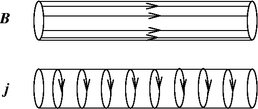
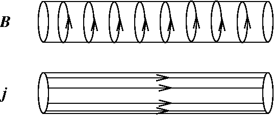
Figure 1: As Maxwell’s equations are linear, the solutions can be superposed. The superposition of a straight flux tube (top left) and a straight current tube (top right) results in a helical flux tube (bottom).

Three-dimensional vector fields may possess chirality (handedness), i.e. their structure may not be mirror symmetric. Concentrating on the magnetic field B, the simplest way to construct such a structure involves the superposition of a magnetic flux tube and a current tube. The result is a twisted tube where both the magnetic field lines and the current lines have a helical structure (Fig.1). This suggests that the helicity can be characterized by the scalar product of B and j; as the latter is proportional to $\nabla\times\mbox{\bf B}$, the current helicity is defined as

$$h_{C}=\mbox{\bf B}\cdot(\nabla\times\mbox{\bf B})$$ (1)

Another quantity characterizing twist, often preferred for theoretical calculations is the magnetic helicity:

$$h_{M}=\mbox{\bf A}\cdot\mbox{\bf B}\equiv\mbox{\bf A}\cdot(\nabla\times\mbox{\bf A})$$ (2)

(To be precise, the above defined $h_{C}$ and $h_{M}$ are helicity densities, helicity being their integral over a finite volume.)

Twist is just one form of helicity. As illustrated in Fig. 2, the twist of a tube or band can be converted into writhe or kink:

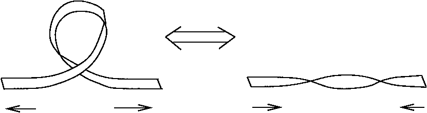
Figure 2: Twist and kink of a magnetic flux tube can be converted into each other, as easily demonstrated by pulling the ends of a kinked paper tape, then pushing them together again.

2 Observations of helical structure on the Sun

The apparent morphology of solar atmospheric structures, especially on $H_{\alpha}$ images, is often vortex-like, twisted or helical. Early claims by ? and ? regarding the predominance of one chirality or another on a given hemisphere were hard to confirm owing to projection effects, a lack of information on 3D structure and large statistical scatter. In any case, the existence of a hemispheric rule of chirality was convincingly demonstrated at least in the case of quiescent prominences and interplanetary magnetic clouds (? ?). Nevertheless, only direct magnetic measurements could provide convincing direct evidence for chirality rules in active regions.

Most determinations of current helicity rely on a constant-$\alpha$ force-free magnetic field model, constructed using the measured line-of-sight field component as lower boundary condition. Such models are based on the assumption that $\nabla\times\mbox{\bf B}=\alpha_{p}\mbox{\bf B}$ where $\alpha_{p}$ is constant. Multiplying this relation by B, it is clear that $\alpha_{p}=h_{C}/B^{2}$ is a normalized measure of current helicity, with a dimension of 1/length. Its meaning is easy to visualize, as $1/\alpha_{p}$ is the length along a flux tube over which he field lines make a full circle around the tube.

Of the possible values of $\alpha_{p}$, a best fit is then chosen by comparing the resulting magnetic field structure to either morphological features seen in solar images taken in $H_{\alpha}$, EUV, etc. (? ?) or, more recently, to the horizontal field components as measured by vector magnetographs (? ?). A third method consists in simply taking the ratio $\alpha_{p}=(\nabla\times\mbox{\bf B})_{n}/B_{n}$, as measured by vector magnetographs, and averaging it over the active region. Results derived by different methods generally agree quite well (? ?; ? ?).

Currently all these methods yield a single mean value of $\alpha_{p}$ over the whole active region. This is because the low S/N ratio of vector magnetograph measurements inhibits a reliable study of current helicity distribution across the plage; for the same reason, usually only pixels with relatively high field strength ($B>100\,$G or so) are used in the determination. It is to be hoped that future improvements in magnetograph sensibility will remedy this situation.

These studies have now firmly established that active region magnetic fields have helical structures, with a higher occurrence of negative helicity in the northern hemisphere. The observations show that the typical average value of the current helicity parameter $\alpha_{p}$ in an active region is on the order of $10^{-8}\,$m^-1 (? ?).

The tilt of the axis of bipolar active regions relative to the E-W direction is generally interpreted as evidence for writhe in the emerging flux tubes giving rise to active regions. The origin of this writhe is well understood: it is the consequence of the Coriolis force acting on the downflows in the flux loop legs (? ?). The sign of current helicity implied by the observed tilts is positive on the northern hemisphere, i.e. opposite to the twist measured in the solar photosphere; its amplitude, however, remains well below the $\alpha_{p}$ values quoted above.

3 The origin of helicity

The basic question regarding the origin of the observed magnetic helicities is whether they are generated after the emergence of the flux loop or the flux emerges already in a helical form. Shearing of the photospheric footpoints of magnetic loops due to differential rotation or smaller scale granular and supergranular motions can, in principle, generate a helicity of right sign (? ?); however, the amount of helicity generated in this way seems to be insufficient to compensate for helicity losses in CME’s (? ?). In addition, in an important paper ? studied the time development of the helicity in young, emerging active regions and found a good correlation between emergence rate and helicity increase. In particular, further increase of helicity ceases once the emergence of the loop, as measured by the increase in footpoint separation and area growth, comes to a halt. This observation seems to settle the issue in favor of a subsurface origin of the observed twist.

There are quite a few subsurface mechanisms which may naturally introduce twist in the structure of emerging flux loops. Such proposed mechanisms include helicity generation by the solar dynamo (? ?) and buffeting of the rising flux tubes by helical turbulent motions (? ?). A further possibility is the effect of Coriolis force on flows in rising flux loops (? ?). As we mentioned above, this process is responsible for the generation of positive writhe in active region flux tubes in the northern hemisphere, and thereby for the observed tilt of active regions. As magnetic helicity is conserved in ideal MHD (? ?), the same process should then also give rise to a twist of opposite sense, so that the net helicity remains constant. The amount of helicity generated by this process, however, is too low to explain the observed values of $\alpha_{p}$. On the other hand, a strongly twisted flux tube can develop a writhe by means of the kink instability. This mechanism should lead to a positive correlation of twist and writhe, in contrast to the helicity conservation argument above. Indeed, recent observations by ? and ? indicate that this mechanism may be important in the case of at least some active regions with unusually high tilt.

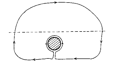
Figure 3: During the rise of a toriodal flux tube (here shown in cross section, hatched) through the convective zone, field lines of the weak external poloidal field may get wrapped around it. After ?.

A further possible theoretical explanation of the observed helicity was proposed by ?, who suggested that the poloidal flux in the solar convection zone (SCZ) gets wrapped around a rising flux tube, as sketched in Fig. 3. ? later showed that this mechanism gives rise to helicity of the same order as what is observed. ? also used their dynamo model to calculate the variation of helicity with latitude over a solar cycle and found that the latitudinal distribution of helicity from their theoretical model is in broad agreement with observational data.

If the magnetic flux in the rising flux tube is nearly frozen, then we expect that the poloidal flux collected by it during its rise through the SCZ would be confined in a narrow sheath at its outer periphery. In order to produce a twist in the flux tube, the poloidal field needs to diffuse from the sheath into the tube by turbulent diffusion. However, turbulent diffusion is strongly suppressed by the magnetic field in the tube. This nonlinear diffusion process was studied in an untwisted flux tube by ?. The model was subsequently successfully applied for sunspot decay (? ?). In a recent paper (? ?) we extended this model by including the poloidal component of the magnetic field (i.e. the field which gets wrapped around the flux tube) and we studied the evolution of the magnetic field in the rising flux tube, as it keeps collecting more poloidal flux during its rise and as turbulent diffusion keeps acting on it.

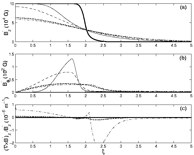
Figure 4: Plots of $B_{z}^{\prime}$, $B_{\phi}^{\prime}$ and $\alpha_{p}$ as functions of $\xi$ for a rising flux tube (case A). The different curves correspond to the profiles of these quantities at the following positions of the flux tube: $0.7R_{\odot}$ (thick solid), $0.85R_{\odot}$ (solid), $0.9R_{\odot}$ (dashed), $0.95R_{\odot}$ (dotted), $0.98R_{\odot}$ (dash-dotted).

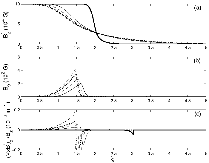
Figure 5: Same as Fig. 4 but the field inside the flux tube is not allowed to decrease below $3B_{e}$ at any height. (Case B)

Consider a straight, cylindrical, horizontal magnetic flux tube rising through the solar convective zone. As all variables in this model depend only on the radial distance $r$ from the tube axis and on time, we study the wrapping of the large-scale poloidal field around the flux tube by considering a radially symmetric accretion of azimuthal field by the flux tube. A further complication is the expansion of the flux tube during its rise, due to the decrease of the external pressure. This expansion is assumed to be self-similar, so that the Lagrangian radial coordinate $\xi$ is related to the Eulerian radius $r$ by $\xi=F(t)r$, where the expansion factor $F(t)$ was taken from thin flux tube emergence models. In the Lagrangian frame, flux density is rescaled as $B^{\prime}_{z}=B_{z}/F^{2}$ and $B_{\phi}^{\prime}=B_{\phi}/F$. With these notations and assumptions, the induction equation takes the form

$$\frac{\partial B^{\prime}_{z}}{\partial t}=F^{2}\frac{1}{\xi}\frac{\partial}{\partial\xi}\left(\eta\xi\frac{\partial B^{\prime}_{z}}{\partial\xi}\right)$$ (3)

$$\frac{\partial B_{\phi}^{\prime}}{\partial t}=F^{2}\frac{\partial}{\partial\xi}\left[\eta\frac{1}{\xi}\frac{\partial}{\partial\xi}(\xi B_{\phi}^{\prime})\right]-F\frac{\partial}{\partial\xi}(vB_{\phi}^{\prime}).$$ (4)

(Note that the advection term appears in the $\phi$ component only, as it does not represent a truly radially symmetric inflow; instead, it is just designed to mimick the effect of the wrapping of poloidal field lines around the rising tube.) Following ?, the magnetic diffusivity $\eta$ is specified in the form

$$\eta=\frac{\eta_{0}}{1+(B/B_{eq})^{2}}$$ (5)

All our calculations are performed for a flux tube of flux $10^{22}\,$Mx and initial field strength $10^{5}\,$G.

Numerical solutions of the equations are presented in Figures 4 and 5. The conclusions drawn from our model hinge on some assumptions, especially concerning the subsurface magnetic field structure in the last phases of the rise of the tube. The field strength in the rising tube, as calculated from thin flux tube emergence models, decreases well below the turbulent equipartition value $B_{e}$ near the surface ($B_{e}^{2}/2\mu_{0}=\rho\overline{v^{2}}/2$). The presence of 3000 G magnetic fields in sunspots is a compelling proof that magnetic fields may never fall to such low values; in fact, at least in photospheric layers, they are at about $3B_{e}$. This is presumably the result of flux concentration processes such as turbulent pumping and convective collapse. Thus, it may be more realistic not to allow the magnetic field to fall below $3B_{e}$. Figures 4 and 5 present results without and with this constraint, respectively.

Inspecting the lower panels of Figures 4 and 5 one finds that the typical value of $\alpha_{p}$ in the internal parts of the flux tube is of order $\sim 10^{-8}\,$m^-1 at a depth of $0.85R_{\odot}$ in both cases. However, as the flux reaches the solar surface, in case A the $B_{\phi}$ component spreads out due to diffusion and its gradient becomes smaller, reducing $\alpha_{p}$ by about one order of magnitude. Only if the magnetic field inside the flux tube remains stronger than the equipartition field (the case B represented in Figure 5) is the $B_{\phi}$ component unable to diffuse inside so that its gradient remains strong and $\alpha_{p}$ is of order $\sim 10^{-8}\,$m^-1 even near the surface. This suggests that our case B may be closer to reality, i.e. during the rise of the flux tube from $0.9R_{\odot}$ to $0.98R_{\odot}$ effective flux concentration processes are at work, keeping the field strength at a value somewhat above the equipartition level.

Note, however, that in the calculations presented here the amplitude and sign of the poloidal field was assumed not to depend on depth. For alternative assumptions, significantly different current helicities may result, so the above conclusion should be treated with proper reservation. Details of the radial dependence of the poloidal field strength may strongly depend on the dynamo model.

A more robust feature of the current helicity distributions, present in all the lower panels of our plots, is the presence of a ring around the tube with a current helicity of the opposite sense. This is clearly the consequence of the fact that on the outer side of the accreted sheath the radial gradient of the azimuthal field, and thus the axial current, is negative. This is an inevitable corollary of the present mechanism of producing twist in active regions. A rather strong prediction of this model is, therefore, that a ring of reverse current helicity should be observed on the periphery of active regions, somewhere near the edge of the plage.

4 Conclusion

One rather strong prediction of our model is the existence of a ring of reverse current helicity on the periphery of active regions. On the other hand, the amplitude of the resulting twist (as measured by the mean current helicity in the inner parts of the active region) depends sensitively on the assumed structure (diffuse vs. concentrated/intermittent) of the active region magnetic field right before its emergence, and on the assumed vertical profile of the poloidal field. Nevertheless, a mean twist comparable to the observations can result rather naturally in the model with the most plausible choice of assumptions (case B).

It is likely that the accretion of poloidal fields during the rise of a flux tube is just one contribution to the development of twist. Its importance may also be reduced by 3D effects: considering the rise of a finite flux loop instead of an infinite horizontal tube, the possibility exists for the poloidal field to “open up”, giving way to the rising loop with less flux being wrapped around it. It is left for later multidimensional analyses of this problem to determine the importance of any such reduction. In any case, the results presented above indicate that the contribution of poloidal field accretion to the development of twist can be quite significant, and under favourable circumstances it can potentially account for most of the current helicity observed in active regions.

This research was carried out in the framework of the Indo-Hungarian Inter-Governmental Science & Technology Cooperation scheme, with the support of the Hungarian Research & Technology Innovation Fund and the Department of Science and Technology of India. K.P. acknowledges support from the ESMN network supported by the European Commission, and from the OTKA under grant no. T043741. P.C. acknowledges financial support from Council for Scientific and Industrial Research, India under grant no. 9/SPM-20/2005-EMR-I.

Bibliography

- Berger, M. 1999, Plasma Phys. Contr. Fusion, 41, B167
- Burnette, A. B., Canfield, R. C., Pevtsov, A. A. 2004, ApJ, 606, 565
- Chatterjee, P., Choudhuri, A. R., Petrovay, K. 2006, A&A, 449, 781
- Choudhuri, A. R. 2003, Sol. Phys., 215, 31
- Choudhuri, A. R., Chatterjee, P., Nandy, D. 2004, ApJ, 615, L57
- DeVore, C. R. 2000, ApJ, 539, 944
- D’Silva, S., Choudhuri, A. R. 1993, A&A, 272, 621
- Fan, Y., Gong, D. 2000, Sol. Phys., 192, 141
- Hale, G. E. 1927, Nature, 119, 708
- Holder, Z. A., Canfield, R. C., McMullen, R. A., Nandy, D., Howard, R. F., Pevtsov, A. A. 2004, ApJ, 661, 1149
- Leka, K. D., Skumanich, A. 1999, Sol. Phys., 188, 3
- Longcope, D. W., Fisher, G. H., Pevtsov, A. A. 1998, ApJ, 507, 417
- López Fuentes, M. C., Démoulin, P., Mandrini, C. H., Pevtsov, A. A., van Driel-Gesztelyi, L. 2003, A&A, 397, 305
- Petrovay, K., Moreno-Insertis, F. 1997, ApJ, 485, 398
- Petrovay, K., van Driel-Gesztelyi, L. 1997, Sol. Phys., 176, 249
- Pevtsov, A. A., Canfield, R. C., Metcalf, T. R. 1995, ApJ, 440, L109
- Pevtsov, A. A., Maleev, V. M., Longcope, D. W. 2003, ApJ, 593, 1217
- Richardson, R. S. 1941, ApJ, 93, 24
- Seehafer, N. 1990, Sol. Phys., 125, 219
- Seehafer, N., Gellert, M., Kuzanyan, K. M., Pipin, V. V. 2003, Advances in Space Research, 32, 1819
- van Driel-Gesztelyi, L., Démoulin, P., Mandrini, C. H. 2003, Advances in Space Research, 32, 1855
- Zirker, J. B., Martin, S. F., Harvey, K., Gaizauskas, V. 1997, Sol. Phys., 175, 27